Figures and data in Making work pay in Croatia: An ex-ante evaluation of two in-work benefits using miCROmod

Cite this article as: S. Bezeredi, M. Ledić, I. Rubil, I. Urban; 2019; Making work pay in Croatia: An ex-ante evaluation of two in-work benefits using miCROmod; International Journal of Microsimulation; 12(3); 28-61. doi: 10.34196/ijm.00206

Article
Figures and data
Jump to

7 figures and 13 tables

Figures

Figure 1

Download asset Open asset

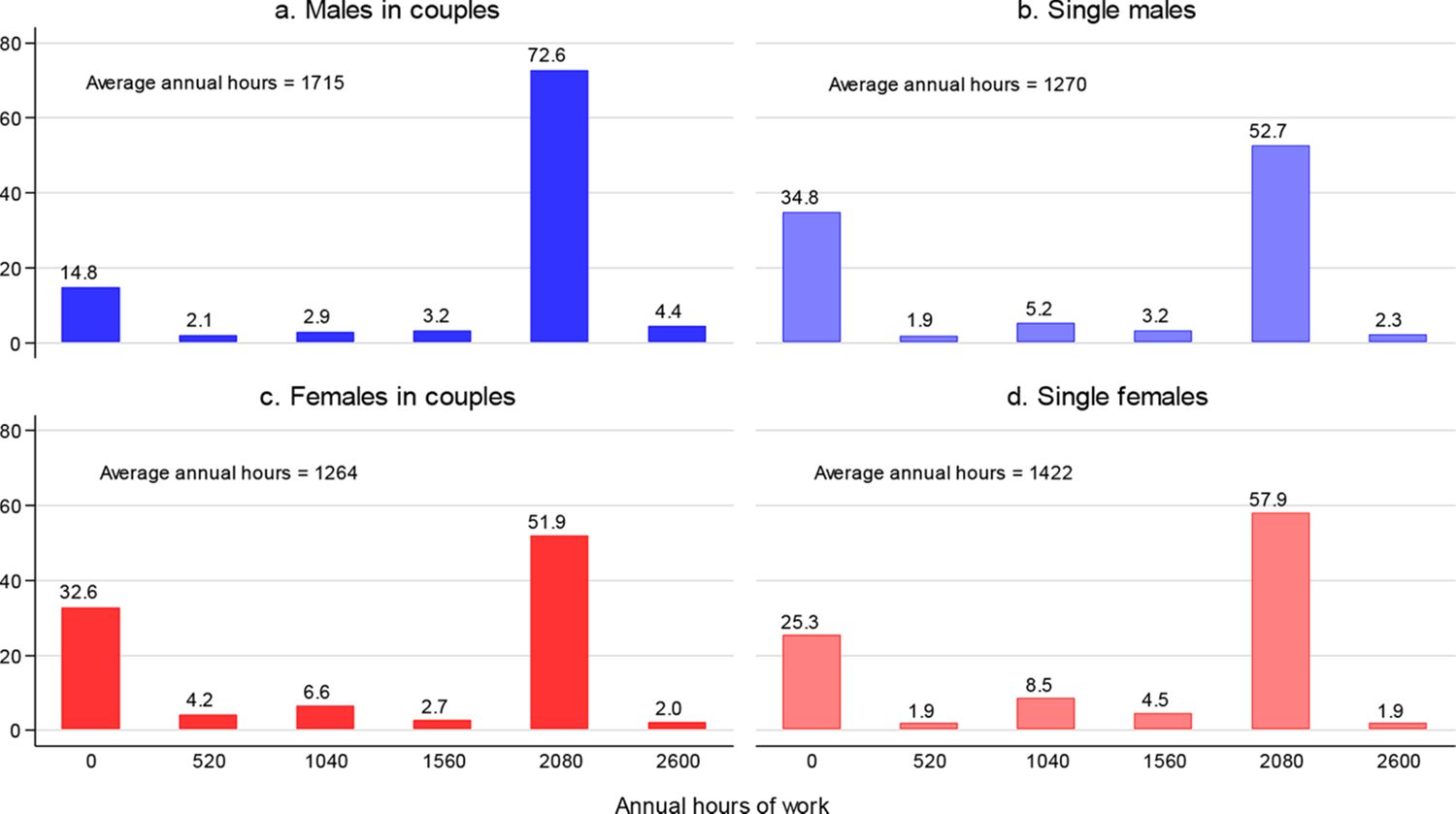
Distributions of discretised hours of work.

Source: Authors’ calculations based on the ILCS 2016 data.

Notes: The bar height measures the share (in %) of persons working the corresponding number of work hours annually. Sample sizes: 1,444 males from couples, 621 single males, 1,444 females from couples, 423 single females.

Figure 2

Download asset Open asset

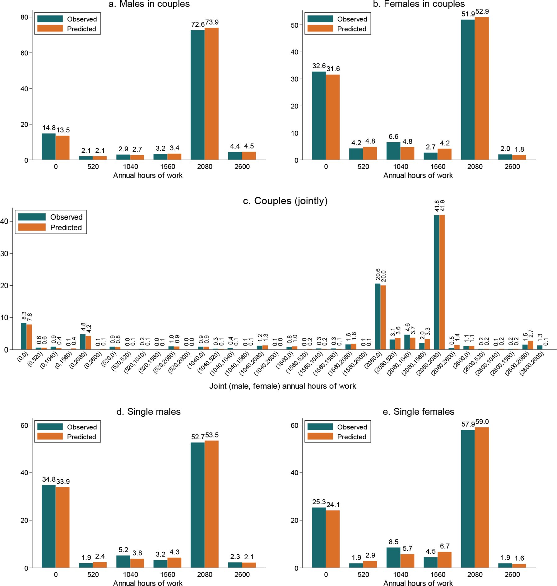
In-sample prediction performance: observed and predicted distributions of hours of work.

Source: Authors’ calculations based on the ILCS 2016 data and the estimates of the labour supply model given in Table 2 (for males and females in couples) and Table 3 (for singles).

Notes: The height of each bar labelled “observed” measures the share of males (panel a), females (panel b) or couples (panel c) observed to work the corresponding number of hours annually in 2015. The annual work hours are the hours after discretisation of their actually observed distribution. The height of each bar labelled “predicted” measures the sample average of the probability to work the corresponding number of hours or, in the case of the joint male-female distribution, the corresponding male-female combination of hours. The probabilities are calculated using the parameters of the labour supply model and data for 2015.

Figure 3

Download asset Open asset

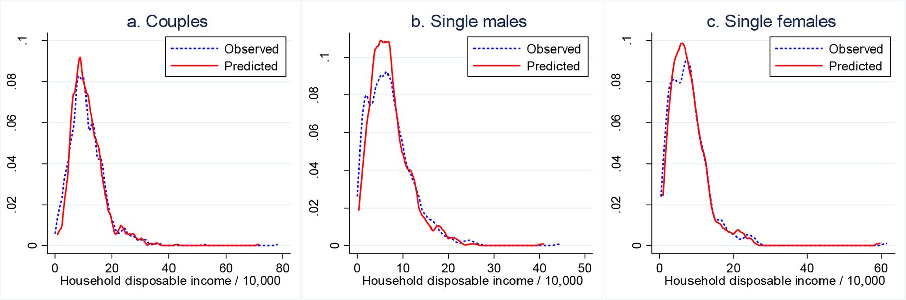
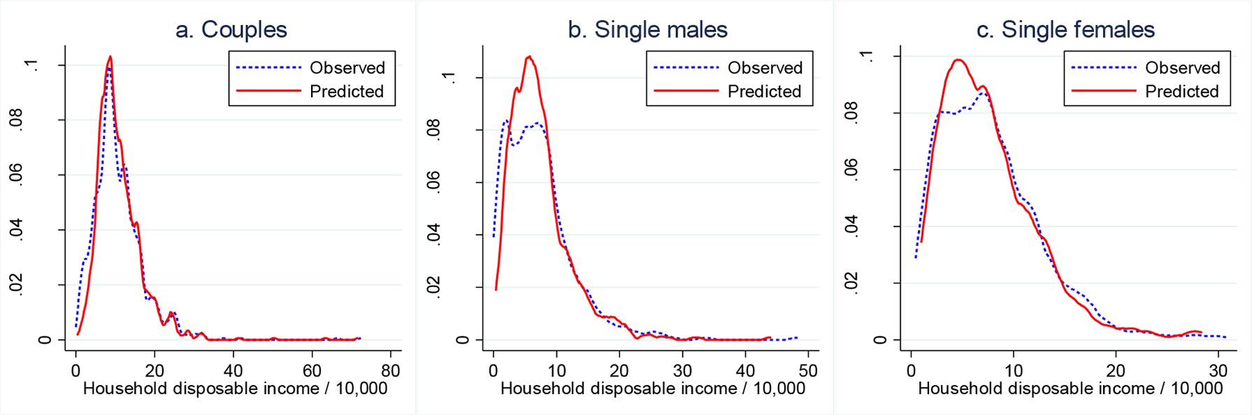
In-sample prediction performance: observed and predicted densities of total household disposable income.

Source: Authors’ calculations based on the ILCS 2016 data and the estimates of the labour supply model given in Table 2 (for males and females in couples) and Table 3 (for singles).

Notes: The densities are kernel estimates. The “observed” density refers to the density of total household disposable income actually observed in the 2015 data. The “predicted” density refers to the density of the expected total household disposable income, where the expectation is taken over the alternative-specific incomes, with the choice probabilities as weights. The choice probabilities are calculated using the parameters of the labour supply model and data for 2015.

Figure 4

Download asset Open asset

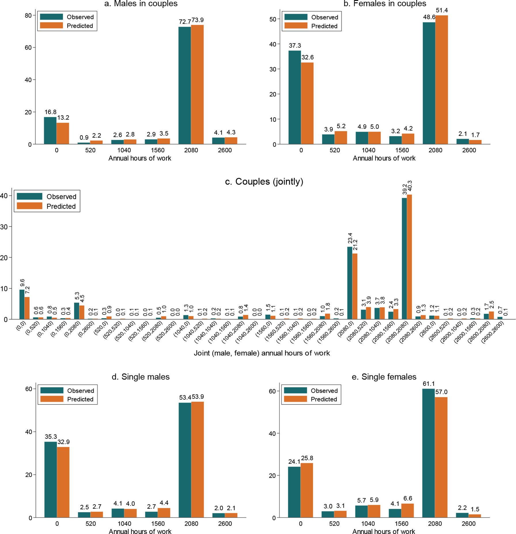
Out-of-sample prediction performance: observed and predicted distributions of hours of work.

Source: Authors’ calculations based on the ILCS 2015 data and the estimates of the labour supply model given in Table 2 (for males and females in couples) and Table 3 (for singles).

Notes: The height of each bar labelled “observed” measures the share of males (panel a), females (panel b) or couples (panel c) observed to work the corresponding number of hours annually in 2014. The annual work hours are the hours after discretisation of their actually observed distribution. The height of each bar labelled “predicted” measures the sample average of the probability to work the corresponding number of hours or, in the case of joint male-female distribution, the corresponding male-female combination of hours. The probabilities are calculated using the parameters of the labour supply model for 2015 and data for 2014.

Figure 5

Download asset Open asset

Out-of-sample prediction performance: observed and predicted densities of total household disposable income.

Source: Authors’ calculations based on the ILCS 2015 data and the estimates of the labour supply model given in Table 2 (for males and females in couples) and Table 3 (for singles).

Notes: The model is estimated on the 2015 data, and the estimated parameters are used to predict the choice probabilities in the 2014 data. These probabilities are used in the calculation of the expected total disposable income for each household in the 2014 data. The density of this income is labelled “predicted”. The density labelled “observed” is the density of actually observed total household disposable income in the 2014 data.

Figure 6

Download asset Open asset

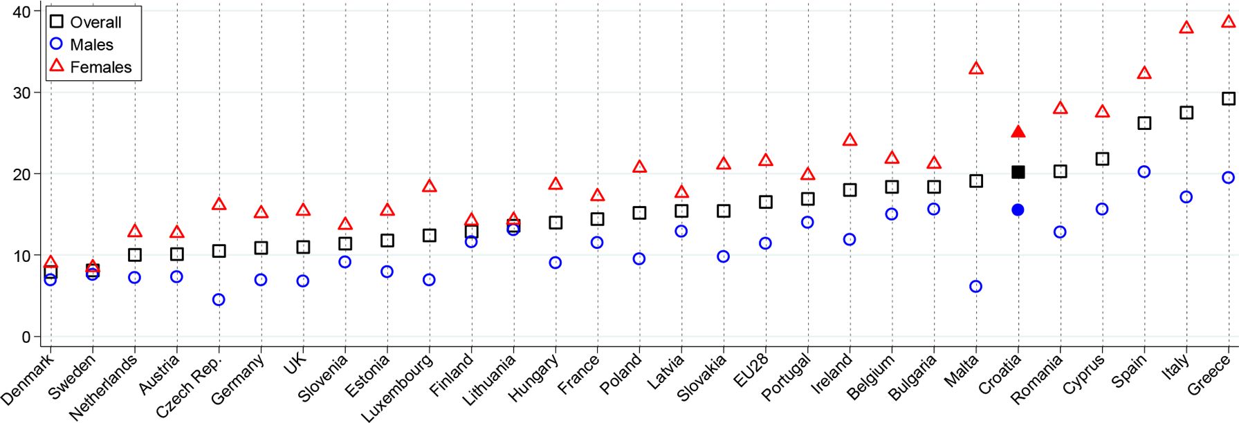
Population aged 20–64 not in employment, education, training, disability or retirement.

Source: Authors’ calculations based on Eurostat data on the unemployment rates, the inactivity rates and the structure of inactivity by the main reason.

Figure 7

Download asset Open asset

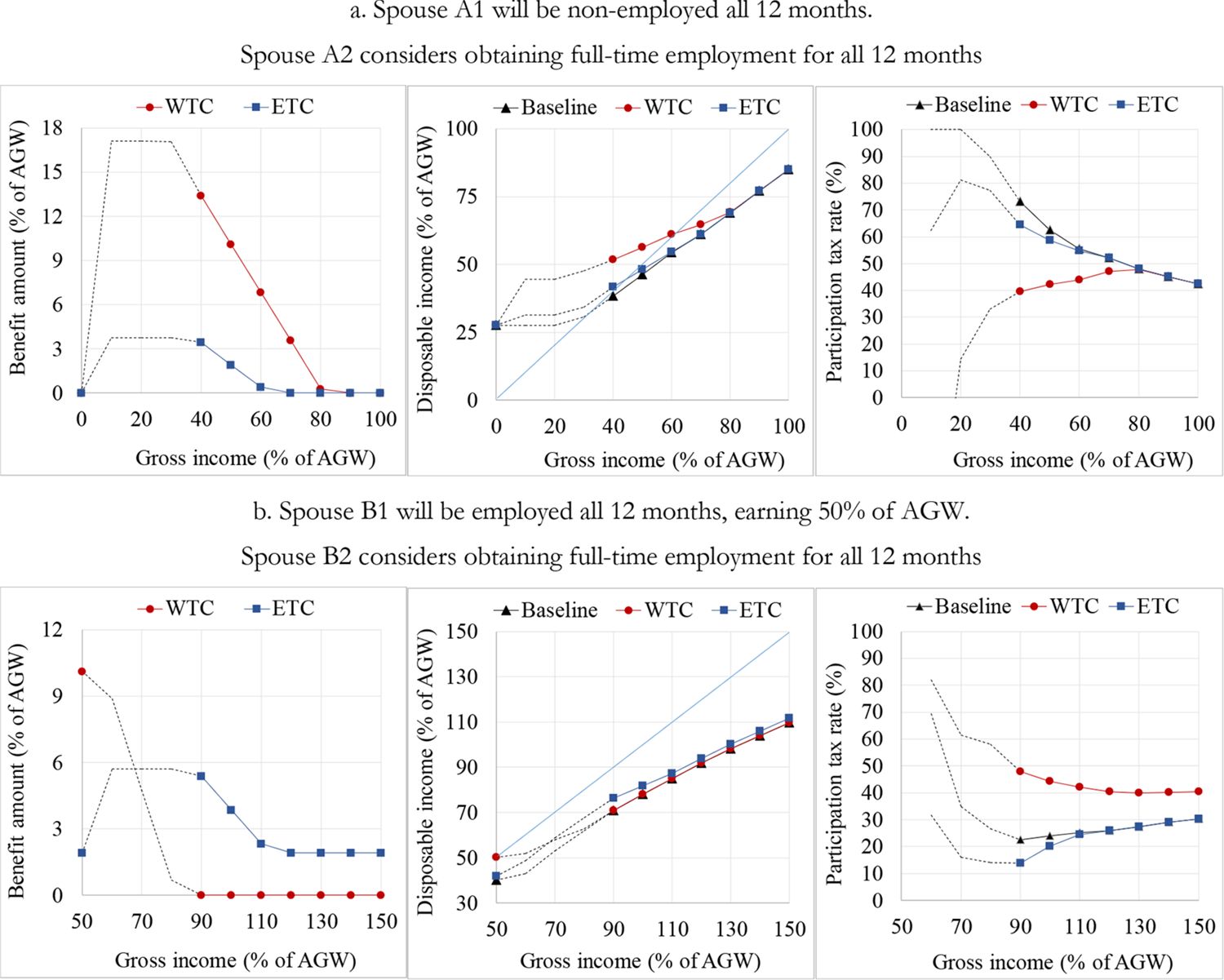
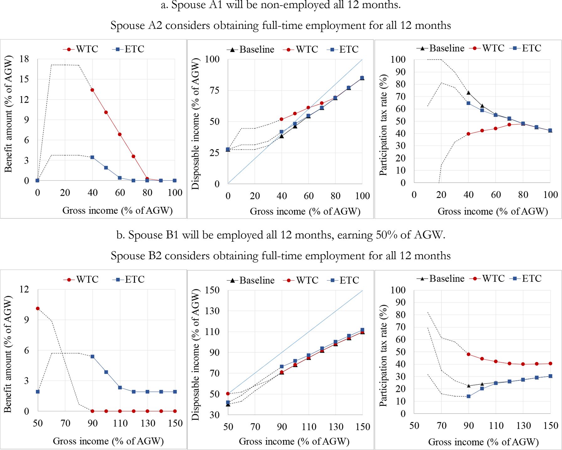
Illustration of the WTC and ETC with two hypothetical couples. a. Spouse A1 will be non-employed all 12 months. Spouse A2 considers obtaining full-time employment for all 12 months b. Spouse B1 will be employed all 12 months, earning 50% of AGW. Spouse B2 considers obtaining full-time employment for all 12 months

Notes: Gross income is the sum of the gross employment incomes of both spouses. The participation tax rate is one minus the change in disposable income taking place upon the transition from non-employment to employment, expressed as a share of gross income that would be earned in the case of employment. In panel a., the benefit amount and disposable income at a gross income of zero are identical for the WTC and ETC scenarios; therefore, the markers overlap, i.e., the one showing the WTC scenario is hidden. In Croatia in 2015, the minimum gross wage for full-time employment was approximately 38% of the average gross wage. Therefore, the actors A2 and B2 cannot be legally employed at a gross wage below the minimum wage. Accordingly, we show the results for gross wages beyond 38% of the AGW (represented by full lines and markers on the graphs). However, for the sake of illustration, the points below 38% of the AGW are also shown (represented by dotted lines on the graphs).

Source: Authors’ simulations using miCROmod.

Tables

Table 1

Discretisation of the distribution of hours of work.

Alternative	Annual hours		Weekly equivalent
Alternative	Interval	Median hours in the interval	Interval	Median hours in the interval
1	[0, 260)	0	[0, 5)	0
2	[260, 780)	520	[5, 15)	10
3	[780, 1300)	1040	[15, 25)	20
4	[1300, 1820)	1560	[25, 35)	30
5	[1820, 2600)	2080	[35, 50)	40
6	≥ 2600	2600	≥50	50

Notes: Each interval is left-closed and right-opened. The weekly equivalents are obtained by dividing the annual hours by 52 (the number of weeks in a year).

Table 2

Estimates of preference and opportunity parameters for couples.

	Parameter	Estimate	Std. err.
Preferences
$C$	$\beta _{C}$	0.464	[0.214]*
$C^{2}$	$\beta _{CC}$	−0.005	[0.002]*
$L_{M}$	$\beta _{0M}$	4.606	[2.858]
$L_{M}^{2}$	$\beta _{MM}$	−0.115	[0.167]
$L_{F}$	$\beta _{0F}$	10.769	[2.506]***
$L_{F}^{2}$	$\beta _{FF}$	−0.434	[0.149]**
$C \times L_{M}$	$\beta _{CM}$	0.023	[0.017]
$C \times L_{F}$	$\beta _{CF}$	0.009	[0.011]
$L_{M} \times L_{F}$	$\beta _{MF}$	0.267	[0.060]***
$L_{M} \times a g e_{M}$	$\beta _{1M}$	−0.188	[0.056]**
$L_{M}\times age_{M}^{2}$	$\beta _{2M}$	0.002	[0.001]**
$L_{M} \times n o . \ o f p r e s c h o o l c h i l d r e n$	$\beta _{3M}$	0.059	[0.083]
$L_{M} \times 1 [h e a l t h l i m i t a t i o n_{M}]$	$\beta _{4M}$	0.401	[0.123]**
$L_{M} \times 1 [s e v e r e \ h e a l t h l i m i t a t i o n_{M}]$	$\beta _{5M}$	0.641	[0.228]**
$L_{F} \times a g e_{F}$	$\beta _{1F}$	−0.204	[0.042]***
$L_{F} \times a g e_{F}^{2}$	$\beta _{2F}$	0.002	[0.000]***
$L_{F} \times n o . \ o f p r e s c h o o l c h i l d r e n$	$\beta _{3F}$	0.200	[0.067]**
$L_{F} \times 1 [h e a l t h l i m i t a t i o n_{F}]$	$\beta _{4F}$	0.194	[0.109]
$L_{F} \times 1 [s e v e r e \ h e a l t h l i m i t a t i o n_{F}]$	$\beta _{5F}$	0.959	[0.231]***
Male opportunity measure
$1 [H_{M} > 0]$	$\gamma _{0M}$	4.164	[1.115]***
$1 [H_{M} > 0] \times a g e_{M}$	$\gamma _{1M}$	−0.211	[0.027]***
$1 [H_{M} > 0] \times e x p e r i e n c e_{M}$	$\gamma _{2M}$	0.180	[0.017]***
Female opportunity measure
$1 [H_{F} > 0]$	$\gamma _{0F}$	3.203	[0.716]***
$1 [H_{F} > 0] \times a g e_{F}$	$\gamma _{1F}$	−0.167	[0.019]***
$1 [H_{F} > 0] \times e x p e r i e n c e_{F}$	$\gamma _{2F}$	0.136	[0.012]***
Male and female opportunity densities
$1 [H_{M} = 2080]$	$\pi _{M}$	2.901	[0.115]***
$1 [H_{F} = 2080]$	$\pi _{F}$	2.865	[0.121]***
Log-likelihood		−2,477.53
No. of couples		1,444

Source: Authors’ estimation using ILCS 2016 data.
Notes: Maximum simulated likelihood estimates with 50 simulations. */**/*** indicate statistical significance at the 10/5/1% level. 1[.] is an indicator variable that equals one if the condition in parentheses is true, and zero otherwise. C is measured in tens of thousands of HRK. L_M and L_F are measured in thousands of hours. Age and experience are measured in years.

Table 3

Estimates of preference and opportunity parameters for singles.

	Parameter	Males		Females
	Parameter	Estimate	Std. err.	Estimate	Std. err.
Preferences
$C$	$\beta _{C}$	0.404	[0.177]*	0.825	[0.237]**
$C^{2}$	$\beta _{CC}$	−0.006	[0.002]**	−0.006	[0.003]*
$L$	$\beta _{L}$	12.797	[3.809]**	27.226	[4.830]***
$L^{2}$	$\beta _{LL}$	−0.586	[0.248]*	−1.365	[0.300]***
$C \times L$	$\beta _{CL}$	0.007	[0.019]	−0.024	[0.026]
$L \times a g e$	$\beta _{1}$	−0.157	[0.045]**	−0.230	[0.061]***
$L \times a g e^{2}$	$\beta _{2}$	0.002	[0.001]**	0.002	[0.001]**
$L \times n o . \ o f p r e s c h o o l c h i l d r e n$	$\beta _{3}$			0.071	[0.256]
$L \times 1 [h e a l t h l i m i t a t i o n]$	$\beta _{4}$	0.776	[0.165]***	0.366	[0.203]
$L \times 1 [s e v e r e \ h e a l t h l i m i t a t i o n]$	$\beta _{5}$	1.413	[0.395]***	0.561	[0.553]
Opportunity measure
$1 [H > 0]$	$\gamma _{0}$	3.267	[1.144]**	4.567	[1.275]***
$1 [H > 0] \times a g e$	$\gamma _{1}$	−0.229	[0.030]***	−0.261	[0.038]***
$1 [H > 0] \times e x p e r i e n c e$	$\gamma _{2}$	0.202	[0.020]***	0.174	[0.028]***
Opportunity density
$1 [H = 2080]$	$\pi$	2.718	[0.183]***	2.614	[0.215]***
Log-likelihood		−550.02		−394.81
No. of individuals		621		423

Source, Authors’ estimation using ILCS 2016 data.
Notes: Maximum simulated likelihood estimates with 50 simulations. */**/*** indicate statistical significance at the 10/5/1% level. 1[.] is an indicator variable that equals one if the condition in parentheses is true, and zero otherwise. C is measured in tens of thousands of HRK. L_M and L_F are measured in thousands of hours. Age and experience are measured in years.

Table 4

Elasticity of the labour supply for couples.

	Elasticity of the probability of participation				Elasticity of the expected work hours
	Males		Females		Males		Females
	Own elasticity	Cross elasticity	Own elasticity	Cross elasticity	Own elasticity	Cross elasticity	Own elasticity	Cross elasticity
All	0.179	−0.010	0.325	−0.030	0.232	−0.017	0.423	−0.046
Income quintile group
first	0.498	0.035	0.677	0.046	0.593	0.037	0.823	0.043
second	0.212	−0.005	0.442	−0.026	0.276	−0.008	0.569	−0.035
third	0.126	−0.013	0.336	−0.017	0.179	−0.016	0.454	−0.027
fourth	0.102	−0.025	0.238	−0.051	0.148	−0.036	0.328	−0.071
fifth	0.072	−0.026	0.166	−0.056	0.109	−0.039	0.237	−0.080
Age
30 or less	0.135	0.003	0.484	−0.015	0.218	0.001	0.699	−0.049
31–50	0.144	−0.007	0.311	−0.033	0.195	−0.014	0.408	−0.048
50 or more	0.285	−0.020	0.314	−0.025	0.341	−0.029	0.382	−0.036
Education
Low	0.344	0.020	0.567	0.012	0.421	0.023	0.690	0.002
Middle	0.180	−0.009	0.339	−0.034	0.237	−0.016	0.446	−0.050
High	0.108	−0.025	0.226	−0.034	0.145	−0.036	0.306	−0.053
Preschool children (age 0–6)
No	0.182	−0.013	0.292	−0.033	0.233	−0.021	0.377	−0.046
Yes	0.171	−0.002	0.425	−0.021	0.231	−0.006	0.575	−0.047
Number of children (age 0–17)
No	0.226	−0.021	0.302	−0.036	0.280	−0.030	0.382	−0.050
1 or 2	0.149	−0.008	0.318	−0.030	0.200	−0.015	0.420	−0.048
3 or more	0.224	0.005	0.444	−0.013	0.287	0.001	0.578	−0.025

Source: Authors’ calculationsbased on the estimates of the labour supply model from Table 2 and the ILCS2016 data.
Notes: For definitions of the elasticities, see Section 4.4. The elasticities are calculated assuming a 10% increase in the gross wage, either the individual’s own (for own elasticities) or that of the partner (for cross elasticities). Income refers to the expected household disposable income equivalised using the modified OECD equivalence scale; the expectation is taken over the 36 alternatives, with the estimated choice probabilities as weights.

Table 5

Elasticity of the labour supply for singles.

	Elasticity of the probability of participation		Elasticity of the expected work hours
	Males	Females	Males	Females
All	0.266	0.276	0.305	0.346
Income quintile
first	0.598	0.695	0.663	0.822
second	0.352	0.364	0.405	0.463
third	0.242	0.319	0.289	0.403
fourth	0.216	0.174	0.252	0.241
fifth	0.150	0.089	0.170	0.132
Age
30 or less	0.294	0.337	0.368	0.517
31–50	0.248	0.263	0.284	0.332
50 or more	0.291	0.272	0.317	0.304
Education
Low	0.316	0.487	0.357	0.557
Middle	0.251	0.307	0.293	0.388
High	0.282	0.200	0.304	0.260
Preschool children (age 0–6)
No	0.266	0.272	0.305	0.342
Yes	–	0.326	–	0.418
Number of children (age 0–17)
No	0.268	0.267	0.309	0.336
1 or 2	0.189	0.298	0.051	0.371
3 or more	–	0.389	–	0.480

Source: Authors’ calculations based on the estimates of the labour supply model from Table 3 and the ILCS 2016 data.
Notes: For definitions of the elasticities, see Section 4.4. The elasticities are calculated assuming a 10% increase in gross wage, either own (for own elasticities) or the partner’s (for cross elasticities). Income refers to the expected household disposable income equivalised using the modified OECD equivalence scale; the expectation is taken over the six alternatives, with the estimated choice probabilities as weights. There are no single males with children aged 0–6 or with three or more children.

Table 6

Parameters of WTC and ETC.

	WTC	ETC
Maximum benefit amount, M	(a)+(b)+(c)+(d)	3,623
(a) Basic element	6,735	–
(b) Lone parent element	6,907	–
(c) Couple element	6,907	–
(d) 1560 hours element	2,784	–
Income threshold, T	22,060	36,360
Withdrawal rate, r	0.41	0.19

Notes: All monetary parameters are expressed in HRK. These values of parameters ensure that the total amount of each benefit given to the sample couples is HRK 300 million in a framework without behavioural effects.

Table 7

Aggregate effects of the WTC and ETC on the labour supply.

	Annual hours of work
	0	520	1040	1560	2080	2600
	Males
a. Baseline	13.36	2.04	2.63	3.39	74.09	4.49
b. WTC reform	13.74	2.18	2.79	3.52	73.42	4.35
c. ETC reform	13.02	2.08	2.80	3.50	74.16	4.45
WTC reform vs. baseline (b – a)	0.37	0.14	0.15	0.14	−0.66	−0.14
ETC reform vs. baseline (c – a)	−0.35	0.04	0.16	0.11	0.07	−0.04
	Females
d. Baseline	30.60	5.34	5.01	4.24	53.00	1.81
e. WTC reform	31.39	5.40	4.99	4.23	52.23	1.76
f. ETC reform	29.43	5.39	5.26	4.43	53.71	1.79
WTC reform vs. baseline (e – d)	0.79	0.06	−0.02	−0.01	−0.77	−0.05
ETC reform vs. baseline (f – d)	−1.17	0.05	0.25	0.19	0.71	−0.03

Source: Authors’ simulations using miCROmod.
Notes: Each figure represents the probability of working a certain number of hours (0, 520, 1040, 1560, 2080 or 2600) in a certain scenario (baseline, WTC reform or ETC reform).

Table 8

The effects of the WTC and ETC on the probability of participation for males and females depending on the employment status of their spouses.

	WTC reform vs. baseline		ETC reform vs. baseline
	Males	Females	Males	Females
Aggregate effect	−0.37	−0.79	0.35	1.17
	a. Type-specific effect on the probability of participation
Spouse not employed	0.38	1.63	0.51	1.38
Spouse employed	−0.74	−1.21	0.27	1.14
	b. Contribution to the aggregate effect
Spouse not employed	0.13	0.24	0.17	0.20
Spouse employed	−0.50	−1.03	0.18	0.97

Source: Authors’ simulations using miCROmod.
Notes: Each figure represents the change (expressed in percentage points) in the probability of participation upon the introduction of the WTC or ETC. The aggregate effect is equal to the effect on the probability of non-participation (zero work hours) reported in the first column of Table 7, multiplied by –1; thus, it measures the change in the probability of participation (rather than non-participation) upon the introduction of the WTC or ETC. Panel (a) displays the changes in the participation probability for males and females depending on whether their spouses are employed or not. In panel (b), the aggregate effect is decomposed into the respective contributions of the two types: the aggregate effect equals the sum of the two contributions. Each contribution is calculated as the product of a type-specific effect from panel (a) and the share of that type in all males or females.

Table 9

Effects of the WTC and ETC on the state budget and employment income.

	Baseline	WTC reform		ETC reform
	Baseline	Without labour supply resp.	With labour supply resp.	Without labour supply resp.	With labour supply resp.
1. Employment income	44,094	44,094	43,756	44,094	44,222
2. Employer SIC	7,353	7,353	7,297	7,353	7,375
3. Employee SIC	8,592	8,592	8,527	8,592	8,617
4. PITS	2,515	2,515	2,507	2,515	2,515
5. Means-tested benefits	1,096	1,096	1,089	1,096	1,082
6. Other benefits	2,341	2,341	2,338	2,341	2,338
7. WTC or ETC	0	300	393	300	316
8. Total taxes = (2)+(3)+(4)	18,460	18,460	18,330	18,460	18,507
9. Total benefits = (5)+(6)+(7)	3,437	3,737	3,820	3,737	3,736
10. Net taxes = (8 – 9)	15,023	14,723	14,510	14,723	14,771
11.Net taxes (vs. baseline)	0	−300	−513	−300	−252

Source: Authors’ simulations using miCROmod.
Notes: Amounts expressed in millions of HRK. SIC – social insurance contributions. PITS – personal income tax plus surtax.

Table 10

Effects of the WTC and ETC on inequality and poverty.

	Baseline	WTC reform		ETC reform
	Baseline	Without labour supply responses	With labour supply responses	Without labour supply responses	With labour supply responses
Gini coefficient	29.30	28.50	28.70	28.90	28.68
Poverty headcount	16.85	14.40	15.39	16.06	15.66
Poverty gap	5.80	4.86	4.70	5.52	5.30
Poverty severity	3.08	2.68	2.44	2.95	2.80

Source: Authors’ simulations using miCROmod.
Notes: All indices are based on the equivalised (OECD scale) household disposable income. The poverty line equals 60% of the overall median.

Table A-1

Descriptive statistics for the variables used in the Heckman selection model.

	Males (N=3543)				Females (N=3823)
	Employed (N=2830)		Non-employed (N=713)		Employed (N=2544)		Non-employed (N=1279)
	Mean	SD	Mean	SD	Mean	SD	Mean	SD
hourly wage	41.97	29.01	–	–	35.97	22.34	–	–
ln(hourly wage)	3.61	0.48	–	–	3.46	0.47	–	–
age	41.44	10.83	43.22	11.62	42.60	10.15	45.02	10.61
education	12.79	2.21	11.86	1.92	13.29	2.63	11.49	2.09
experience	18.71	11.00	12.36	11.60	18.27	10.87	8.99	11.10
1[urban settlement]	0.21	0.41	0.19	0.39	0.25	0.43	0.15	0.36
1[health limitation]	0.10	0.30	0.22	0.42	0.13	0.34	0.22	0.41
1[severe health limitation]	0.02	0.14	0.08	0.27	0.02	0.14	0.06	0.24
1[in consensual union]	0.65	0.48	0.46	0.50	0.71	0.45	0.83	0.38
no. of children aged 0–6	0.24	0.56	0.14	0.49	0.18	0.46	0.24	0.59
no. of children aged 7–14	0.33	0.73	0.20	0.57	0.33	0.63	0.37	0.73
other market income	0.21	0.22	0.15	0.20	0.27	0.24	0.22	0.22
social insurance income	0.06	0.09	0.07	0.11	0.06	0.10	0.07	0.11

Source: Authors’ calculations based on the ILCS 2016 data.
Notes: N is the number of observations. Hourly wage is in HRK. Age, education and experience are in years. Other market income and social insurance income are in tens of thousands of HRK, and both are divided by the square root of the number of household members. 1[.] is an indicator variable that equals one if the condition in brackets is true, and zero otherwise.

Table A-2

Estimates of the Heckman selection model for the prediction of missing wage rates.

	Males		Females
Estimate	Std. err.	Estimate	Std. err.
Wage equation
age	0.000	[0.010]	−0.019	[0.010]*
age²/100	−0.006	[0.012]	0.009	[0.011]
education	0.092	[0.004]***	0.094	[0.004]***
experience	0.025	[0.006]***	0.042	[0.005]***
experience²/100	−0.030	[0.011]*	−0.056	[0.011]***
1[urban settlement]	0.138	[0.020]***	0.141	[0.018]***
constant	2.238	[0.173]***	2.237	[0.177]***
Selection equation
age	−0.119	[0.030]***	−0.021	[0.024]
age²/100	−0.005	[0.035]	−0.084	[0.028]**
education	0.130	[0.015]***	0.137	[0.012]***
experience	0.240	[0.014]***	0.199	[0.008]***
experience²/100	−0.291	[0.031]***	−0.270	[0.016]***
1[urban settlement]	−0.030	[0.074]	0.093	[0.067]
1[health limitation]	−0.548	[0.084]***	−0.227	[0.071]**
1[severe health limitation]	−0.909	[0.144]***	−0.559	[0.143]***
1[in consensual union]	0.255	[0.085]**	0.021	[0.072]
no. of children aged 0–6	−0.018	[0.068]	−0.446	[0.056]***
no. of children aged 7–14	−0.026	[0.055]	−0.195	[0.044]***
other market income	0.355	[0.155]*	−0.174	[0.128]
social insurance income	−0.089	[0.318]	−0.458	[0.271]
constant	1.476	[0.569]**	−0.394	[0.495]
rho	−0.266	[0.078]**	0.446	[0.096]***
sigma	0.421	[0.006]***	0.402	[0.008]***
lambda	−0.112	[0.033]**	0.179	[0.041]***
No. of censored observations	713		1,279
No. of uncensored observations	2,830		2,544
Log-likelihood	−2,693.9		−2,685.7

Source: Authors’ estimation based on the ILCS 2016 data.
Notes: Maximum likelihood estimates. */**/*** indicate statistical significance at the 10/5/1% level. 1[.] is an indicator variable that equals one if the condition in brackets is true, and zero otherwise. Hourly wage is in HRK. Age, education and experience are in years. Age, education and experience are in years. Other market income and social insurance income are in tens of thousands of HRK, and both are divided by the square root of the number of household members.

Table B-1

Descriptive statistics for the variables used in the estimation of the labour supply model.

	Couples (N=1444)				Singles (N=1044)
	Males (N=1444)		Females (N=1444)		Males (N=621)		Females (N=423)
	Mean	SD	Mean	SD	Mean	SD	Mean	SD
consumption (C)	11.21	6.27	11.21	6.27	7.10	4.88	7.85	5.50
leisure hours (L)	7.04	0.78	7.50	0.97	7.49	0.98	7.34	0.91
no. of preschool children	0.36	0.65	0.36	0.65	0.00	0.00	0.07	0.27
age	44.84	8.24	41.70	8.29	42.49	10.26	42.67	10.05
experience	20.68	8.97	14.40	10.38	15.62	11.21	16.37	11.25
1[health limitation]	0.13	0.34	0.14	0.35	0.15	0.35	0.16	0.37
1[severe health limitation]	0.03	0.17	0.03	0.18	0.04	0.19	0.02	0.14
1[H>0]	0.85	0.35	0.67	0.47	0.65	0.48	0.75	0.44
1[H=2080]	0.73	0.45	0.52	0.50	0.53	0.50	0.58	0.49

Source: Authors’ calculations based on the ILCS 2016 data.
Notes: N is the number of observations. Consumption is measured in tens of thousands of HRK. Leisure hours are annual and are measured in thousands of hours. 1[.] denotes an indicator variable that equals one if the condition in brackets is true, and zero otherwise.

Data and code availability

The data is proprietary. The data (referred to as ILCS in the paper) were collected by the Croatian Bureau of Statistics and are available only to Croatian scientific researchers, upon signing a special agreement.

The model is proprietary, with executable also not available.

Download links

A two-part list of links to download the article, or parts of the article, in various formats.

Downloads (link to download the article as PDF)

Article PDF

Download citations (links to download the citations from this article in formats compatible with various reference manager tools)

BibTeX
RIS

Open citations (links to open the citations from this article in various online reference manager services)

Mendeley

Distributions of discretised hours of work.

In-sample prediction performance: observed and predicted distributions of hours of work.

In-sample prediction performance: observed and predicted densities of total household disposable income.

Out-of-sample prediction performance: observed and predicted distributions of hours of work.

Out-of-sample prediction performance: observed and predicted densities of total household disposable income.

Population aged 20–64 not in employment, education, training, disability or retirement.

Discretisation of the distribution of hours of work.

Estimates of preference and opportunity parameters for couples.

Estimates of preference and opportunity parameters for singles.

Elasticity of the labour supply for couples.

Elasticity of the labour supply for singles.

Parameters of WTC and ETC.

Aggregate effects of the WTC and ETC on the labour supply.

The effects of the WTC and ETC on the probability of participation for males and females depending on the employment status of their spouses.

Effects of the WTC and ETC on the state budget and employment income.

Effects of the WTC and ETC on inequality and poverty.

Descriptive statistics for the variables used in the Heckman selection model.

Estimates of the Heckman selection model for the prediction of missing wage rates.

Descriptive statistics for the variables used in the estimation of the labour supply model.

Downloads (link to download the article as PDF)

Download citations (links to download the citations from this article in formats compatible with various reference manager tools)

Open citations (links to open the citations from this article in various online reference manager services)