The Hypothetical Household Tool (HHoT) in EUROMOD: a new instrument for comparative research on tax-benefit policies in Europe
- Herman Deleeck Centre for Social Policy, University of Antwerp, Belgium
- European Commission, Joint Research Centre (JRC), Spain
- Institute for New Economic Thinking at the Oxford Martin School, University of Oxford, UK
- Institute for Social and Economic Research, University of Essex, UK
- Organisation for Economic Co-operation and Development (OECD), France
- Bank of Italy, Italy
- Formerly Herman Deleeck Centre for Social Policy, University of Antwerp, Belgium
- Federal Public Service Social Security, Belgium
- Article
- Figures and data
-
Jump to
- Abstract
- 1. Introduction
- 2. The complementarity of population-based microsimulation and hypothetical household simulations
- 3. The integration of hypothetical household simulations in EUROMOD
- 4. Potential applications of HHoT
- 5. Conclusion
- Footnotes
- Appendix 1
- References
- Article and author information
Abstract
This paper introduces the Hypothetical Household Tool (HHoT), a new extension of EUROMOD, the tax-benefit microsimulation model for the European Union. With HHoT, users can easily create their own hypothetical data, which enables them to better understand how policies work for households with specific characteristics. The tool creates unique possibilities for an enhanced analysis of taxes and social benefits in Europe by integrating results from population-based microsimulations and hypothetical household simulations in a single modelling framework. Furthermore, the flexibility of HHoT facilitates an advanced use of hypothetical household simulations to create new comparative policy indicators in the context of multi-country and longitudinal analyses. In this paper, we highlight the main features of HHoT, its strengths and limitations, and illustrate how it can be used for comparative policy analysis.
1. Introduction
In this paper, we introduce the Hypothetical Household Tool (HHoT). HHoT is an extension of the European tax-benefit microsimulation model EUROMOD that allows the user to generate hypothetical households with a wide range of characteristics in a flexible environment. These households can subsequently be used as an input database for EUROMOD to assess how tax-benefit policies work and interact with each other. Traditionally, EUROMOD is used for analysing the distributive, labour market and budgetary impact of tax-benefit policies and policy changes. To do so, detailed and representative data on persons and households are required. With the HHoT extension, users can create their own hypothetical data, which allows them to better understand how policies work for households with specific characteristics, while giving them full control over the characteristics of interest. This creates unique possibilities for an enhanced analysis of taxes and social benefits in Europe by integrating results from hypothetical household simulations and population-based microsimulations in a single modelling framework. The flexibility of HHoT facilitates the simulation of a range of comparative indicators such as the marginal effective tax rate, the net replacement rate and unemployment or inactivity traps for a large set of hypothetical households in a comparative setting.
In what follows, we first briefly elaborate on the differences and synergies between microsimulation based on representative microdata, and hypothetical household simulations in the context of analysing tax-benefit policies. Subsequently, we introduce the EUROMOD framework and the HHoT extension. In the third part we illustrate several ways in which HHoT can be used for policy analysis. This paper accompanies a paper by Gasior and Recchia (2019), which presents baseline results of HHoT for 2017 policies in the EU.
2. The complementarity of population-based microsimulation and hypothetical household simulations
With hypothetical household simulations, also known as model-family analysis or standard simulations, the researcher specifies detailed characteristics of a limited set of households. In the case of tax-benefit simulation, these households and their specifications are used to compute the households’ tax liabilities and benefit entitlements as well as detailed information on income components and total disposable income. In contrast to hypothetical household simulations, population-based microsimulation makes use of representative microdata (eg, collected in a household survey or from tax registers and social security registers) for which tax liabilities and benefit entitlements are computed, thus taking into account the full heterogeneity of household characteristics in the population[1].
Hypothetical household simulations have several strengths that make them an attractive tool for policy analysis. (1) Given that users can fully control the characteristics of hypothetical data, it is possible to generate indicators of the institutional functioning of tax-benefit systems that are independent of cross-national or longitudinal variations in population characteristics (eg, regarding work incentives, benefit generosity, income adequacy, targeting, replacement rates, implicit equivalence scales), thus allowing for a comparative analysis of the institutional structure of tax-benefit systems that isolates the effect of tax-benefit policies from the composition of the population. This is particularly relevant when evaluating policies that can have a non-negligible impact on the characteristics of the population. For instance, when studying work incentives of tax-benefit policies, the incidence of certain household types and work patterns themselves are likely to be influenced by the work incentives that flow from these tax-benefit policies. If this results in a relatively low incidence of household compositions and work behaviours that are financially discouraged, population-based simulations might not be able to reveal, or risk to downplay, the discouraging incentives that result from the tax-benefit system, given the low incidence of these situations in the data. Hypothetical household simulations are particularly useful for describing tax-benefit systems across countries with different policy designs. Microsimulation analysis using population-based data may put less weight on policies that encourage certain demographic behaviours (eg, two-earner orientated policies), whereas this becomes more clear when using similar household types across countries. (2) For the same reason, it is possible to illustrate in an accessible way for very simple (or rather complex) households how tax-benefit systems operate and how policies interact with each other. This allows users to grasp more easily how tax-benefit systems (or potential policy reforms) work and facilitates the validation of tax-benefit calculations. (3) Given that users generate their own hypothetical households, it is possible to assess the functioning of tax-benefit policies when adequate representative household data are lacking. For instance, this applies to studying households that are too rare in household samples for a reliable statistical analysis (eg, single-parent families with three or more children under the age of 7); and to situations when very up-to-date simulations are required (representative survey data or register data typically become available with quite some delay); or when aspects of policies require variables which are unavailable in the dataset (eg, on health or assets).
By their specific nature, hypothetical household simulations are not fit for distributive analysis and for drawing conclusions about the population as a whole (see also Immervoll et al. (2004) for a discussion of some limitations of hypothetical household analysis). In other words, they cannot show the aggregated impact of policies or policy reforms at the population level, eg, in terms of poverty, inequality, budgetary effects, or overall labour market participation. This can only be done on the basis of representative household data (either through a sample or population data) and, when analysing the impact on eg, labour supply, in combination with a behavioural model. Thus, population-based microsimulation is required whenever researchers want to say something about the effect on a population, rather than describing the institutional architecture of tax-benefit systems. It stands out, though, that in many cases hypothetical household simulations and population-based microsimulations are complementary to each other. For instance, when studying a reform related to the progressivity of taxation it is useful to see how progressive personal income taxes are in relation to the population under study and how a change impacts different parts of the population. However, given that results depend on the composition of the population under consideration, when comparing countries it is useful to complement such an analysis with an analysis of how different systems would perform for the same set of (hypothetical) households. Both approaches can also generate different indicators of closely related phenomena (eg, hypothetical household simulations of the extent to which social assistance benefits reach the poverty threshold, jointly with a study of social assistance coverage and non-take-up). So far though, most comparative studies either make use of one approach or the other, rather than using them jointly in a synergetic way, because models are either based on population-based or on hypothetical household data. With HHoT integrated in EUROMOD, the same tax-benefit model can be used for both population-based microsimulation and hypothetical household simulations, in a single framework, implying that it is much easier to combine the strengths of both approaches. Furthermore, EUROMOD allows doing this in a comparative context (multiple countries and/or years) as well as analysing the effect of policy reforms rather than just the status quo.
EUROMOD is the cross-country tax-benefit model for the European Union, used by both academics and policy analysts. Many countries also have national models (eg, IZAΨMOD for Germany, TAXBEN for the UK, FASIT for Sweden, etc.) (Li et al., 2014). Population-based microsimulation studies require the availability of (comparable) representative household microdata with sufficient information to assess tax liabilities and benefit entitlements. Such data have only been available since the late 1990s in many EU countries. The advantage of running microsimulation models on representative household data is the possibility to carry out distributional analyses, and to show the effects of tax-benefit policies and tax-benefit reforms on the distribution of work incentives and disincentives across the population and on government budgets (Li et al., 2014; Sutherland and Figari, 2013and Van Mechelen and Verbist, 2005).
With regard to hypothetical household simulations, several databases have been created which contain for a limited set of hypothetical households tax-benefit simulations that span an extended time period and cover a wider range of countries. Examples include the CSB Minimum Income Protection Indicators database CSB-MIPI (Van Mechelen et al., 2011) and the Social Assistance and Minimum Income Protection Interim Dataset SaMIP (Nelson, 2013). The main drawback of these databases is that they contain information for a limited number of cases, and simulations are hard-wired: one cannot assess what would happen if the policy rules were changed. Furthermore, updating is typically done in a more ad-hoc way given that it is rather demanding to generate the data (see, for instance, Marx and Nelson (2013), for a more detailed description and applications of the use of these databases). An exception to these two limitations is the OECD Tax-Benefit Calculator, which is specifically designed to carry out hypothetical household simulations for tax-benefit policies, in a flexible and user-friendly environment (eg, Immervoll, 2010; OECD, 2014)[2]. Recently the OECD developed a tax-benefit web calculator that enables users to quickly see and compare the tax liabilities and benefits entitlements in 40 OECD and EU member states. Family types, the income situation and the percentage of the average wage can be changed easily. Previous versions of EUROMOD already included a basic tool to simulate tax-benefit rules for hypothetical households. Compared to the OECD tool, HHoT/EUROMOD has the advantage that it allows for integrating population-based and hypothetical household simulations in a single modelling framework, and that it is more flexible in terms of specifying household characteristics and the simulation of policy reforms. At the same time, this flexibility implies that the tool is also less accessible than the OECD online calculator for those not familiar with EUROMOD.
3. The integration of hypothetical household simulations in EUROMOD
EUROMOD is both a software platform and the tax-benefit microsimulation model for the EU (Sutherland and Figari, 2013). From the beginning, the aim of EUROMOD was to develop an accessible model that facilitates comparative research (Immervoll and O’Donoghue, 2009). As a result, EUROMOD is characterised by a drive for comparable policy modelling and the use of largely comparable and detailed microdata (now mostly EU-SILC). The scope of the simulated tax-benefit policies is limited to parameters for which the household data provide sufficient information. Consequently, policies that require longitudinal information on contribution records are not simulated (in particular contributory pensions). The model is built and maintained by a group of researchers from universities, research institutes and ministries from all EU countries under the coordination of a team of researchers at the University of Essex[3]. Continuing support from the European Commission ensures regular updates of the model (policy rules) and the data (Sutherland and Figari, 2013). The cross-country comparability, the flexibility of the modelling software, the regular updates and the standardised validation of the model are important features to meet the increasing demand from users of hypothetical household simulations.
For many years, EUROMOD contained a very basic hypothetical household generator. This tool was mostly used for the validation of the model, even though it could also be used to understand tax-benefit systems by separating the effect of tax-benefit rules from the effects of the populations structure (Berger et al., 2001). However, it was not very flexible: there were strong limits on the extent to which household characteristics could be manipulated. To enlarge the possibilities of hypothetical household simulations with EUROMOD, we designed the Hypothetical Household Tool – HHoT. The tool, based on the experience of experts in both population-based microsimulation and hypothetical household analysis, was developed as part of the InGRID-project, an infrastructure project funded by the European Union’s seventh Framework Programme (Hufkens et al., 2016). A first version of EUROMOD incorporating HHoT was released to the user community in December 2017, covering policies from 2009 up to 2017.
HHoT is a EUROMOD extension for generating hypothetical households. It can be accessed within the standard EUROMOD user interface under Applications. The user generates a EUROMOD dataset by specifying households and the characteristics of the household members. Once the households are generated, the dataset can be used within EUROMOD to simulate tax liabilities and benefit entitlements as well as detailed information on income components and total disposable household income for the hypothetical households. This EUROMOD output dataset can thereafter be analysed with software of the user’s choice. By defining the group at risk (eg, employed, unemployed, inactive) in the tool, HHoT follows a ‘risk-type approach’ for hypothetical household simulations: the user defines the characteristics of the households on the basis of generic assumptions, subsequently the simulation model ‘decides’ which policies are applicable (cf. Van Mechelen et al., 2011). When running the simulation model, the hypothetical households are treated as if they were real households in a microdataset. Thus, the user needs to make sure to specify the personal and household characteristics such that the hypothetical household is eligible for the taxes and benefits of interest.
The tool allows the user to specify the characteristics of households for all parameters that are used in the EUROMOD model. To make it more user-friendly, a distinction is made between standard and advanced variables. In the case of standard variables the user manipulates a limited number of characteristics and makes use of default values for all other variables. In the case of advanced variables, users have full control over all characteristics that are used in the simulations. The user can define in a flexible way the characteristics of the hypothetical households: in contrast to typical hypothetical household data or simulations, multi-generational households and complex household compositions can be generated, while also characteristics such as tenure status, region of residence, sector of employment, etc., can be changed. The possible employment statuses are employee, self-employed, unemployed, pensioner, student/pupil or preschool. All numeric variables (eg, age, earnings or housing costs) can be specified either as a single value or as a range. When specifying a range, the same hypothetical household is reproduced for each value within the range while keeping all other characteristics constant. It is also possible to include a ‘reference table’ to specify quantitative variables as a percentage of a value in the reference table rather than in absolute terms. For instance, gross earnings can be specified as a percentage of the country and year specific minimum wage, the average wage or another reference wage. The tool allows users to include their own reference tables. Hypothetical households can be given recognisable names and can be saved for later use.
It is easy to run EUROMOD for the same set of hypothetical households simultaneously for multiple policy years and countries. As is the case for population-based microsimulations, users have full control over the simulated policies and can decide to ‘switch on’ or ‘switch off’ policies, or simulate the effect of a policy reform or ‘policy swap’. Furthermore, advanced users can revise the EUROMOD baseline by introducing new policy parameters and new policies that require data that are not available in the microdata, but can be taken into account when specifying the characteristics of the hypothetical households in HHoT. A user manual of HHoT is available online[4].
The flexibility of HHoT allows users to easily create numerous hypothetical households (especially when specifying a range for more than one numeric variable) for several countries and years. However, it is essential to always assess whether the assumptions hold equally across countries or policy years. Users should also be aware that compared to other hypothetical household simulations (eg, CSB-MIPI), results based on HHoT are not always the same, largely because of differences in the level of detail with which some policy measures are modelled (see Hufkens et al., 2016; Marchal et al., 2019). As a user of HHoT, it is therefore important to be aware of the extent to which policies are simulated in EUROMOD.
4. Potential applications of HHoT
The possibilities of policy relevant uses of HHoT are numerous. In this section we describe briefly four examples of how HHoT can create an added-value for the analysis of tax-benefit policies. The examples are drawn from various strands of research and make use of different household specifications to show the flexibility of HHoT. In the first example we show how hypothetical household simulations can complement insights from population-based microsimulations in the case of a simple policy reform. In subsequent illustrations, we only present results based on hypothetical household simulations, even though there could be complementarities with population-based microsimulations. In the second example, we identify the gross wage level that is required to reach the level of the poverty line in a selection of EU-countries. This exercise makes use of the option to vary flexibly the range of gross income for each household member. Then we calculate implicit equivalence scales of the tax-benefit system in four EU-countries, showing that with HHoT it is also very easy to change other household characteristics, such as household composition. In the last exercise we show the marginal effective tax rates for all EU-countries and explain some of the differences across countries and income levels. Unless specified otherwise, we assume that the hypothetical households live in the capital region (insofar regional policies are relevant and simulated in EUROMOD).
4.1. Example 1: Combining population-based microsimulation and hypothetical household simulations to measure the impact of a policy change
In Germany, like in many other countries, children in single parent families face a relatively high poverty risk (Commission, and E, 2014; Eurostat, 2017; Lenze, 2014). Reforming child benefits (Kindergeld) can reduce the at-risk-of-poverty rate for families with children. We simulate a simple reform aimed at reducing child poverty in single parent families in Germany to illustrate how hypothetical household simulations and population-based microsimulations can jointly help to design and understand policies. With the current child benefit system, the level of child benefit depends on the rank of the child in the family. In 2016, the level of the child benefit was 190 euro per month for the first and second child, 196 euro per month for the third and 221 euro per month for all other children. The benefit is paid to one of the parents. Child benefits are non means-tested, non-taxable benefits. At the same time, child benefits are part of the definition of income that is used for the income test of Unemployment Benefit II (Arbeitslosengeld II), social assistance related benefit (Sozialhilfe) and general social assistance. Apart from child benefits, families with children are entitled to a tax allowance for children. This allowance is only granted to parents if it is more beneficial to receive the tax allowance than the child benefit and is mostly relevant to higher income households. A third benefit that aims at improving the financial situation of families with children is the additional child benefit (Kinderzuschlag). The additional child benefit is, in contrast to the Kindergeld, means-tested. To be eligible for the additional child benefit, households also need to be eligible for Kindergeld. (eg, Gallego Granados and Harnisch, 2017). In the reform that we simulate below, we focus on the design of the child benefits only. The reform scenario is budgetary neutral compared to the baseline.
In the reform scenario we abolish the current system based on ranks and replace it by a fixed amount for each child. Children in two-parent households receive 180 euro per month while children in single parent households are entitled to 248 euro per month. As illustrated in Table 1, we simulate the effect of the reforms for four different households, while varying the labour market status of the adults. In households with only one child, the child is 8 years old, in households with three children, the children are aged 5, 8 and 12. We first present the effect of the reform on the situation of households in which all adults work full time at the minimum wage, and subsequently on the situation in which all adult household members are inactive[5].
Summary of hypothetical households used in example 1
| Demographic composition | Labour market status adults | |
|---|---|---|
| Couple (2 earners) with child (8 years) | Employee – full time at minimum wage | Inactive |
| Single with child (8 years) | ||
| Couple (2 earner) with 3 children (5, 8 and 12 years) | ||
| Single with 3 children (5, 8 and 12 years) | ||
The table below shows the effect of the policy change for the four hypothetical households in the case that adult household members are at work. From Table 2 it can be seen that the financial situation of single parent households improves after the reform while disposable income decreases in two parent households irrespective of the number of children.
Net disposable income and different income components for four hypothetical households, minimum wage, 2016
| Two adults with 1 child | One adult with 1 child | Two adults with 3 children | One adult with 3 children | |||||
|---|---|---|---|---|---|---|---|---|
| Baseline | Reform | Baseline | Reform | Baseline | Reform | Baseline | Reform | |
| Total | Total | Total | Total | Total | Total | Total | Total | |
| Gross earnings | 2,947 | 2,947 | 1,473 | 1,473 | 2,947 | 2,947 | 1,473 | 1,473 |
| Total taxes | 220 | 220 | 70 | 70 | 220 | 220 | 70 | 70 |
| SIC employee | 602 | 602 | 301 | 301 | 602 | 602 | 301 | 301 |
| Means-tested benefits | 0 | 0 | 0 | 0 | 0 | 0 | 410 | 410 |
| Non-means-tested Child Benefit | 190 | 180 | 190 | 248 | 576 | 540 | 576 | 744 |
| Disposable income | 2,315 | 2,305 | 1,293 | 1,351 | 2,701 | 2,665 | 2,089 | 2,257 |
-
Source: own calculations based on EUROMOD H1.0+ and HHoT.
Because child benefits are not taxed in Germany and the sociodemographic and labour market characteristics of the simulated hypothetical households are unchanged, Table 2 shows that the benefit reform does not interact with any other part of the tax-benefit system. However, this is not the case for all households. If we change the labour market status of adults in the hypothetical households from ‘employee’ to ‘inactive’, there is an interaction between the non-means-tested child benefit and means-tested benefits. For all households illustrated in Table 3, the reformed child benefit does not result in a changed disposable income. The increase or decrease of the child benefit is fully compensated by a lower or higher Unemployment Benefit II[6]. The income test of the Unemployment Benefit II considers income from employment, pensions and most benefits, including the child benefit (but not the additional child benefit).
Net disposable income and different income components for four hypothetical households, inactive, 2016
| Two adults with 1 child | One adult with 1 child | Two adults with 3 children | One adult with 3 children | |||||
|---|---|---|---|---|---|---|---|---|
| Baseline | Reform | Baseline | Reform | Baseline | Reform | Baseline | Reform | |
| Total | Total | Total | Total | Total | Total | Total | Total | |
| Gross earnings | 0 | 0 | 0 | 0 | 0 | 0 | 0 | 0 |
| Total taxes | 0 | 0 | 0 | 0 | 0 | 0 | 0 | 0 |
| SIC employee | 0 | 0 | 0 | 0 | 0 | 0 | 0 | 0 |
| Means-tested benefits | 1,096 | 1,106 | 861 | 803 | 1,082 | 1,118 | 886 | 718 |
| Non-means-tested Child benefit | 190 | 180 | 190 | 248 | 576 | 540 | 576 | 744 |
| Disposable income | 1,111 | 1,111 | 876 | 876 | 1,658 | 1,658 | 1,462 | 1,462 |
-
Source: own calculations based on EUROMOD H1.0+ and HHoT.
Tables 2 and 3 show the income components of some hypothetical households, illustrating the possible impact of the reform. The hypothetical household simulations make it easier for researchers and policy-makers to understand how the tax-benefit system operates and how the policies interact with each other. Besides, they help researchers and policy-makers to grasp the effect on vulnerable groups that might be underrepresented in the microdata. However, the hypothetical households are not representative for the population. Using a representative sample of the population we calculate the first-order poverty effects of this reform. Table 4 shows poverty headcounts for the baseline and the reform scenario and the difference between the two. Even though the hypothetical household simulations make clear that for some household types disposable income would be substantially increased, the overall (first order) effect on poverty in Germany is not significant. In contrast, the poverty risk of persons living in single parent households decreases significantly at the 90% confidence level, which was the objective of the reform. For persons living in households consisting of two adults and at least one child there is a small, but significant increase in the poverty risk. Focussing on the at-risk-of poverty rate we could conclude that this reform improves the income situation of lone parents with low incomes. HHoT however, allowed us to easily disentangle the effects for active and inactive households and to see the interaction between the child benefits and the means-tested benefit that might be hidden in microsimulation results based on population-data.
At-risk-of-poverty rate of persons living in Germany, by family type, 2016
| Baseline | Reform | Difference | ||||
|---|---|---|---|---|---|---|
| Change | Standard error | 90% confidence interval | ||||
| Lower bound | Upper bound | |||||
| Population | 15.15 | 15.19 | 0.04 | 0.04 | –0.02 | 0.11 |
| One adult with children | 25.04 | 24.28 | –0.75 | 0.44 | –1.48 | –0.03 |
| Two adults with children | 11.53 | 11.75 | 0.21 | 0.12 | 0.02 | 0.41 |
-
We use a fixed poverty line at 60% of the median equivalised disposable income in the baseline.
-
Source: own calculations based on EUROMOD H1.0 and EU-SILC 2014, full sample design information is not available. For estimating the standard errors and confidence intervals, we take account of clustering within households and the covariance between the simulated scenarios (Goedemé, 2013; Goedemé et al., 2013).
4.2. Example 2: How much should one earn to have an income above the at-risk-of-poverty threshold?
In the EU, the at-risk-of-poverty indicator is one of the headline indicators for monitoring poverty and social exclusion. Given that the threshold is set at 60 percent of the national median equivalent disposable household income, it may be difficult to grasp the kind of living standard that is feasible in each member state with an income at the level of the threshold (Goedemé et al., 2019). By using the flexibility of HHoT, it is relatively easy to identify at which wage level a household can have a disposable income at the level of the poverty threshold. This is helpful for further contextualising the at-risk-of-poverty indicator, ie, to make clear what the implications are of using a relative poverty threshold specified in this way. Also, more information on the required gross wage level to reach the at-risk-of-poverty threshold could help to better understand quantitative analyses of (cross-country variations in) in-work poverty. As the simulations below show, the required wage does not only depend on the level of the poverty threshold, but also on the applicable tax liabilities and benefit entitlements. Importantly, when interpreting the results it should be kept in mind that wage levels vary in non-negligible ways in the population (eg, by gender and level of education). This implies that it would be worthwhile to complement the analysis with an alternative set of reference wages.
The approach is very similar to first estimating budget constraints, and subsequently selecting the gross wage which corresponds with the relevant disposable household income (see Gasior and Recchia (2019) for HHoT baseline results for budget constraints in the EU). In a first step we calculate the 60% at-risk-of-poverty threshold on the basis of EU-SILC, with net incomes simulated by EUROMOD[7]. In a second step, we use HHoT and EUROMOD to calculate the disposable income for hypothetical households earning a predetermined percentage of the average wage, which we vary between 60% and 200%. Average gross wages per full-year, full-time equivalent employee refer to 2014 and were downloaded from the OECD database (OECD, 2017). In a third step we identify the gross wage level which corresponds with a disposable income at, or just above, the level of the poverty threshold. As illustrated in Table 5, simulations are carried out for a hypothetical single-person household consisting of a 35 years old male, working full time. The second hypothetical household is a married couple, 35 years old, both working full time. They have two children aged 5 and 8 years old. For the couple-household, we assume both partners are working, and we vary the gross income of both partners from 60% to 200% of the average gross wage. To do this, we imported a separate table in HHoT containing the average gross wages that we downloaded from the OECD online database. Different combinations of the gross wages of both parents are possible; in this exercise we select the income that results in a total disposable household income closest to, but above the poverty threshold[8].
Summary of hypothetical households used in example 2
| Demographic composition | Labour market status adults |
|---|---|
| Single | Employee(s), full time, wage varying from 60% to 200% of average gross wage*[ |
| Couple (2 earners) with 2 children (5 and 8 years) |
-
*
Although we show only one outcome, different combinations of the wages of both partners are possible.
Figure 1 shows the gross income, presented as a percentage of the average wage (OECD, 2017), that is required to reach a disposable income at the level of the at-risk-of-poverty threshold in each country and for the two hypothetical households. In Poland, Estonia, France and Hungary a single person working full time requires a gross income of around 80% of the average wage or more to reach the threshold. In contrast, in Portugal, Italy, Ireland and Greece 60% of the gross average wage suffices to reach an income just above the poverty line. Despite the relative character of the poverty threshold, this is quite a substantial difference. A similar observation can be made for two-earner couples (both working full time) with two children, even though countries score differently as compared to single-person households. While a single person in Hungary should earn about 85% of the average gross wage to reach the threshold, a couple with two children requires a total level of earnings of about 150% of the average gross wage, although the at-risk-of-poverty threshold of a household with two children is 2.1 times as high as the threshold for a single-person household. Compared to the other countries, the (relatively small) difference between the gross wage for a single person and the total gross wage for a couple with two children is remarkable. This shows how the Hungarian tax-benefit system favours couples with children compared to singles (see also Example three below). At the other extreme, in Portugal a couple with two children should earn about 130% of the average gross wage, while 65% of the average gross wage suffices for a single-person household. In Hungary an important part of the increase in disposable income is due to an increase in benefits, whereas in Portugal the impact of benefits is rather small. Also, the effect of the tax system (through joint taxation for couples such as in France, or tax advantages for families with children such as in Italy) can explain differences between countries. A recent similar exercise, done by the OECD on ‘working hours needed to exit poverty’ (OECD, 2019), leads to a comparable conclusion that the design of tax-benefit policies is of great importance when comparing low-income families across countries. More specifically, it is the variation in the implicit equivalence scale of tax-benefit policies which drives the variation in the additional gross wage required by couples with children as compared to single person households to have a net income above the poverty line, a topic to which we turn in the next example.
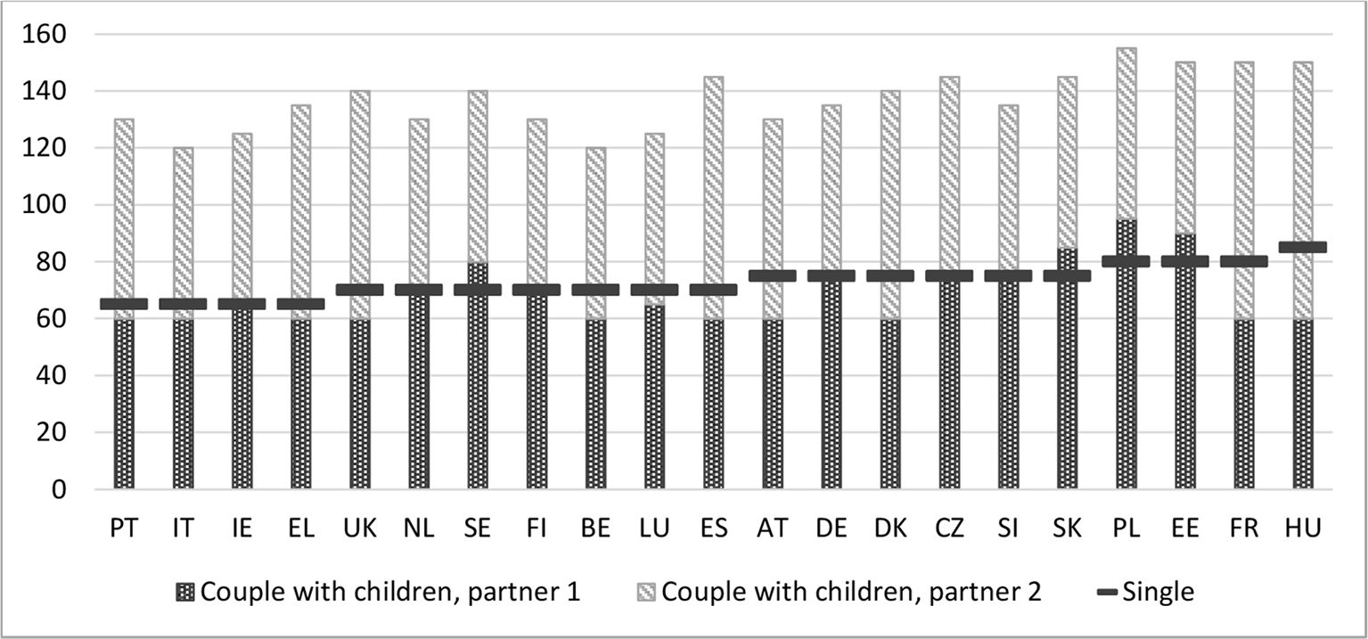
Gross wage needed to reach the at-risk-of-poverty line, as a percentage of the average gross wage per full-year full-time equivalent employee, for a hypothetical family , 2014.
Source: own calculations using EUROMOD H1.0+ and HHoT; poverty threshold and average wages based on EUROMOD calculations using EU-SILC. Note: countries sorted from lowest to highest percentage of the gross average wage needed to reach a disposable income at the level of poverty threshold for a single-person household. The selection of countries is based on availability in EUROMOD and availability of the average gross wage (for 2014 in the OECD online database at the time of writing).
4.3. Example 3: Implicit equivalence scales
Microsimulations based on population data could show how the net incomes of persons living in different household types compare to each other and how, on average, the level and composition of incomes vary. However, these comparisons are limited by the fact that hours worked and wage levels tend to be partially determined by household composition. This implies that it is difficult to judge from these results alone how tax-benefit systems support different household types. For this reason, it can be revealing to calculate ‘implicit equivalence scales’ based on hypothetical data. For the purposes of this exercise, we define the implicit equivalence scale of a tax-benefit system as the extent to which a tax-benefit system treats multi-person households of different size and composition more favourably than a single person household with the same level of gross earnings, in terms of taxes to be paid and eligibility for receiving social benefits. It is typically measured as the ratio of the disposable income of two households that have the same gross wage and similar other characteristics, except for the demographic composition of the household. This shows how policies work in their pure form, and can help to better understand, for instance, the distribution of poverty risks by household type. The calculations are similar to those done in the previous exercise, but now we compare more directly incomes between household types with a similar level of gross income. Further breakdowns can show how not only the level, but also the composition of net incomes differs by household type as a result of tax-benefit policies such that one can identify the policies that drive the implicit equivalence scales.
We calculate implicit equivalence scales for hypothetical households living in Belgium (Flanders), Italy (Lombardia), Greece (capital region) and Hungary (capital region), and take account of the relevant regional policies. The household types included in the analysis in terms of demographic composition and labour market status are displayed in Table 6. For this exercise, the income ranges are based on the average wages calculated using the EUROMOD microdata files (based on EU-SILC). When comparing net incomes between two household types, wages are kept constant. In principle it is desirable to keep also all other characteristics ‘constant’, in spite of the changing composition of the household. Given the availability and setup of housing-related benefits in some countries, housing costs are an important issue in this context. In principle, one could opt for keeping housing costs constant across household types, but this is often not a realistic assumption. Therefore, in this example we started from the level of housing costs that were estimated in another project. More in particular, we made use of the housing cost associated with renting an adequate dwelling on the private market at the 30th percentile of the distribution of housing costs for the relevant household composition, in the relevant region (Van den Bosch et al., 2016). In the case of a more in-depth analysis, it would be worthwhile to undertake sensitivity tests with alternative assumptions regarding housing costs, as we will show below.
Summary of hypothetical households used in example 3
| Demographic composition | Labour market status adults (one-earner families) | |||
|---|---|---|---|---|
| Single | Inactive | Employee, 50% of average EU-SILC wage | Employee, 100% of average EU-SILC wage | Employee, 200% of average EU-SILC wage |
| Couple | ||||
| Single with child of 10 years old | ||||
| Couple with child of 10 years old | ||||
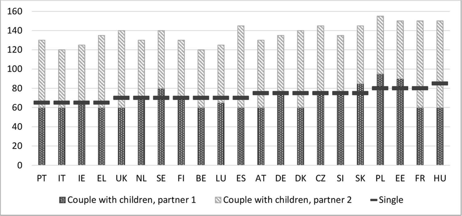
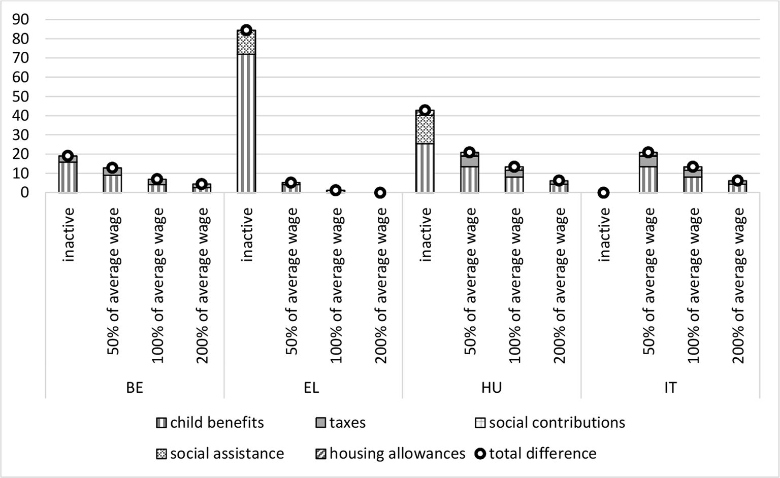
In Figure 2, we show the net income of three household types as a percentage of the net income of a single-person household, having the same level of gross earnings. The households are one-earner households, in the case of couples one partner is assumed to be inactive on the labour market. With HHoT it is easy to make variations for more complex households, but we limit ourselves in this illustration to households with one child. Several observations stand out. First, when looking at differences within countries between different levels of earnings, it is clear that implicit equivalence scales are generally above one and higher for inactive persons and for households with lower wages[9]. This probably has a mitigating effect on poverty for multi-person households living on a low income, even though the size of the effect will vary by the poverty measure used[10]. In contrast, in all four countries included in Figure 2, the implicit equivalence scale at 200% of the average wage is broadly similar to the implicit equivalence scale for households with earnings at 100% of the average wage. While in Greece and Hungary equivalence scales are higher for inactive households as compared to working households earning 50% of the average wage (both for adding a partner or a child), in Belgium the implicit equivalence scale for adding an inactive partner is lower than the scale for adding a partner in a working low-income household (without a child). Second, countries vary strongly in the level of implicit equivalence scales, and the ranking of the four countries differs substantially depending on the household composition under consideration. It is noteworthy that in Italy adding a partner to a single-person household does not make a difference for the tax-benefit system, while adding a child does make a difference. For working families in Belgium and Hungary the implicit equivalence scales of the tax-benefit system are higher for an additional partner as compared to a child, while in Greece and Italy it is the other way around. This shows how the tax-benefit systems across the four countries result in different outcomes in the degree to which they support (or do not support) households with a different demographic composition. Apart from showing how these tax-benefit systems operate, more insight into implicit equivalence scales can also help to better understand varying patterns of poverty and inequality.

Net income for three household types expressed as a percentage of the net income of a single-person household with the same gross wage, but without children, 2014.
Note: Positive values for taxes and social contributions indicate that a household with a child pays less in taxes or social contributions, or receive higher tax credits. Source: own calculations using EUROMOD H1.0+ and HHoT; average wage based on EUROMOD calculations using EU-SILC.
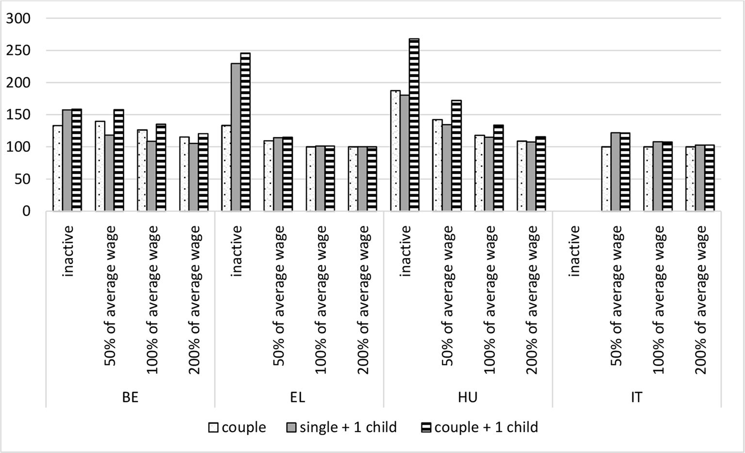
It is also interesting to see which part of the tax-benefit system contributes to the observed implicit equivalence scales. Therefore, in Figures 3 and 4 we describe the different income components that increase the income for a family with a child compared to a family without a child (note that given our focus on child-related tax-benefit generosity, we use the income of a couple without a child in the denominator in Figure 4). More specifically, it shows the difference in the level of each income component (when adding a child), expressed as a percentage of the net income of a similar household without a child, at a similar level of gross earnings. Not surprisingly, child benefits tend to account for most of the difference, while social contributions are no different for households with a child as compared to those without a child. Additional advantages for a single-person households with a child can include both support directed to lone parents specifically, or to households with children more generally. As an exception, for inactive households in Belgium and households earning 50% of the average gross wage in Greece the increase of the net income is mostly due to a higher level of social assistance benefits, especially for single-parent households, compared to single-person households the difference in social assistance in the tax-benefit package is much smaller for couples. Even though the contribution of personal income taxes is significant at higher levels of earnings (especially for couples with a child), it is relatively small, and non-existent in Greece. In Hungary the housing allowance also varies by household composition, resulting in higher benefits for households with a child.

Tax-benefit package for a child in a single parent household, income components expressed as a percentage of the net income of a single parent household without children, 2014.
Source: own calculations using EUROMOD H1.0+ and HHoT; average wage based on EUROMOD calculations using EU-SILC.

Tax-benefit package for a child in a couple parent household, income components compared to the net income in a couple household without children, 2014.
4.4. Example 4: Work incentives
Another area where hypothetical data can be of use is the analysis of work incentives. One way to look at tax-benefit systems is to analyse to what extent they encourage their workforce to take up a job (work incentive on the extensive margin) and to what extent they encourage to work/earn more (work incentive on the intensive margin). In this example, we focus on the marginal effective tax rate (METR) which measures the (dis)incentive to work/earn more, expressed as the share of an earnings increase that is taxed away due to higher social insurance contributions, higher taxes, or the loss of benefit entitlement. We assume a 3% earnings increase in our calculations using the methodological approach suggested by Jara and Tumino (2013). METRs usually take values between 0 and 100, indicating respectively high work incentives when individuals keep the full earnings increase and low incentives when individuals lose the full earnings increase. However, certain aspects of the tax-benefit system might also lead to higher or lower values. We visualise how different elements of the tax-benefit system react to the 3% earnings increase.
All results are based on a single-person household assuming full-time employment of 40 hours per week (cf. Table 7). Country-specific average monthly gross earnings levels are calculated using EU-SILC 2015 data and updated to 2017 using country-specific uprating factors (see Supplementary data for estimated average wages and Gasior and Recchia, 2019 for more detailed information). The person is assumed to live in rented accommodation with housing costs of 20% of the average earnings. As is the case for previous examples, we assume full take-up of benefits as well as full compliance in reporting incomes to tax authorities in all countries.
Summary of hypothetical households used in example 4
| Household composition | Labour market status |
|---|---|
| Single | Employee, full time with between 80% and 120% of the EU-SILC average wage (in 1% steps). |
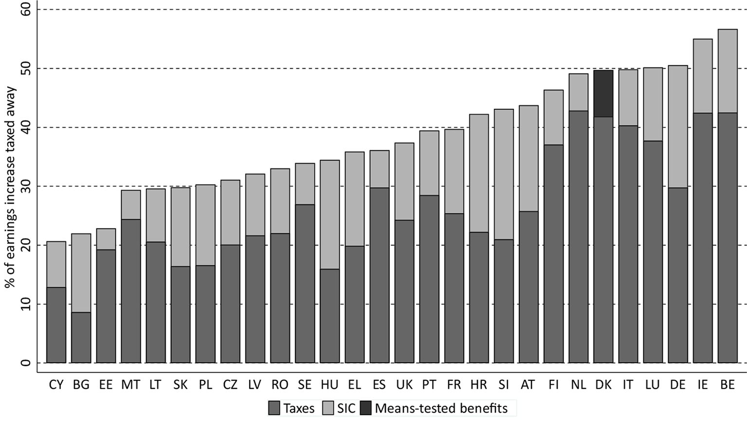
Figure 5 shows (unweighted) average METRs for earners with 80% to 120% (in 1% steps) of average earnings decomposed by taxes, social insurance contributions and benefits. The reason for averaging over 41 cases either side of the mean instead of using the example of an average earner is based on the sensitivity of METRs which can differ a lot between an average earner and someone earning slightly above or below average earnings. This is due to kinks in the tax and benefit schedule, where an earnings increase of 3% more can lead to a significant increase in taxes/social insurance contributions (SIC) or the loss of tax credits or benefits in some countries. Thus, using the average METR of a certain earnings range produces results that are more in line with results based on representative data (see Supplementary data in Gasior and Recchia, 2019).

Decomposition of average METRs for a single person household at earnings levels from 80% to 120% of average earnings by income component, 2017 policy system.
Source: own calculations using EUROMOD H1.0+ (Gasior and Recchia, 2019). Note: SIC = social insurance contributions. Countries are ranked by the percentage of marginal earnings increase taxed away. Policy system 2017 refers to the status quo on 30th of June 2017. Results are based on the assumption of full tax-compliance and full benefit take-up.
Across countries, increases in net earnings are lower than increases in gross earnings due to higher taxes and social insurance contributions. The incentive to earn more is very high in Cyprus, Bulgaria and Estonia, where only about 20% of the earnings increase is lost due to higher taxes and social insurance contributions. Belgium and Ireland are the countries with the highest work disincentives for earnings between 80% and 120% of average earnings. While taxes explain most of the overall level of METRs across countries, social insurance contributions play a similarly important role in Bulgaria, Hungary and Slovenia. Denmark is the only EU country where average earners are still eligible for means-tested benefits (housing benefit and green check) which are reduced when their earnings increase.
While this sheds light on how tax-benefit systems differ in their (dis)incentive to increase working hours/earnings, it is important to keep in mind that incentives can be quite different by earnings levels. We select three countries – Cyprus, Hungary and Belgium – to discuss such differences (see Figure 6). Cyprus represents the countries with the lowest METRs on average and Belgium the countries with the highest METRs (see Figure 5). Hungary represents a group of countries with flat tax system which leads to a quite different picture of METRs at different earnings levels.

Decomposition of METRs at different earnings levels in Cyprus, Hungary and Belgium by income component, 2017 policy system.
Source: own calculations using EUROMOD H1.0+ (Gasior and Recchia, 2019). Note: Policy system 2017 refers to the status quo on 30th of June 2017. Results are based on the assumption of full tax-compliance and full benefit take-up. Level of gross earnings refers percentage of average gross earnings.
Results for Cyprus show relatively low METRs across all income levels except for people with very low earnings. This, however, corresponds to a very specific case in which the baseline earnings represent roughly the minimum wage and the 3% earnings increase leads to earnings above this level. While earnings below the minimum wage are disregarded from the income test for the Guaranteed Minimum Income (GMI), this is not the case for the earnings increase which leads to a slightly smaller benefit amount which creates a high disincentive to work more. All other income groups have incomes above the GMI and hence, are no longer eligible to receive the means-tested benefit. While the deducted SIC of the earnings increase amount to 7.8% of gross earnings across all income groups, only average and above earners are liable to income tax (which subsequently leads to higher METRs). The income tax paid for the earnings increase is progressive, starting at 18% for average earners, and going up to 28% for those with earnings that are twice as high. Nevertheless with the exception of earnings above 150% of average earnings, METRs for earnings above the Minimum Wage are substantially lower than in other countries.
In Belgium on the other hand, incentives to increase wages are relatively low across the earnings distribution with more than 50% of the earnings increase being taxed away. Disincentives are especially high for those with 50% of average earnings due to the high level of social insurance contributions. While the contribution of the income tax increases relatively smoothly up to earnings levels of 125% of average earnings, the contribution of SIC to the METRs is highest for those with 45%–70% of average earnings. This is due to the work bonus which has two parts. The first part is a reduction of SIC, the second part is a tax bonus for monthly gross earnings below € 2,510. Higher earnings lead to a lower work bonus and hence to a slightly higher income tax than before the earnings increase. In other words, when the work bonus is reduced, this reduction does not only apply to the increase in earnings, but to total earnings, which is why the METR is particularly high at this level of earnings.
The picture is quite different in Hungary due to the flat tax system. In relative terms, taxes and SIC deductions are the same across earnings levels (even for those with earnings below the minimum wage). Only certain household types (eg, households with children) are eligible for tax allowances and are subject to lower deductions. In contrast to Cyprus and Belgium, low earnings are not exempted from contributions. This creates the same METR of 35% for all earnings levels. While increases in earnings are largely taxed away by the income tax system in Belgium and Cyprus, SIC play a relatively more important role in Hungary.
This example illustrates the usefulness of hypothetical household data for a better understanding of tax and benefit systems and their implicit work (dis)incentives. The selected country cases demonstrate different levels of METR and the contribution of different tax and benefit elements. It furthermore highlights the importance of taking different earnings levels into account rather than just focusing on average earnings. Even with this simple one-person household example, results are quite different by country and earnings levels. The possibilities to expand such analysis are unlimited by for example focusing on different household compositions and analysing the role of tax allowances and means-tested benefits for these households.
5. Conclusion
With HHoT, EUROMOD now includes a new tax-benefit hypothetical household generator that is freely accessible. The tool is unique in that it is very flexible, yet user-friendly, and – as part of EUROMOD – allows for comparable population-based microsimulations and hypothetical household simulations in an integrated framework. Given that EUROMOD covers all EU Member States, for an increasing number of policy years, the tool has great potential to substantially contribute to (comparative) research in tax-benefit policies. In addition, EUROMOD is supported by a network of experts, responsible for regular updates and validations of the tax-benefit simulation model, ensuring the quality and timeliness of the simulations. In this paper, we introduced HHoT and described its potential for novel research in tax-benefit policies and for producing policy indicators. The uses and the advantages of the tool are manifold. HHoT can enhance tax-benefit analyses and studies of poverty and inequality with illustrations of how policies work and interact with each other in practice. It can also illustrate how proposed policy reforms and reform ideas would work and interact with other policies. Second, it can help users to create (new) policy indicators that keep the composition of the population constant across time and countries, for instance on benefit adequacy and generosity, targeting, implicit equivalence scales and work incentives (for an example of a new indicator, see Penne et al. (2020)). Thirdly, HHoT can be used to go beyond the possibilities of the microdata to study the operation and impact of policy parameters for which variables are lacking in the microdata or in cases where specific households are underrepresented in the microdata. An additional advantage for EUROMOD specifically, is that HHoT helps to validate the tax-benefit algorithms in the model in a very detailed way and without the constraints of data availability. Finally, it is also a valuable tool for introducing new users to EUROMOD and helping them setting the first steps in microsimulation modelling.
Undoubtedly, the main strengths of HHoT are the flexibility in defining hypothetical households and the ease with which comparisons across time and countries can be made. However, users should be aware that it is always necessary to reflect upon the validity of assumptions and the quality of the simulations made, especially in the case of comparative research, and not be tempted to jump all too quickly to (policy) conclusions. With this caveat in mind, we hope that users will quickly embrace the potential that HHoT offers to generate new insights into the functioning and impact of tax-benefit policies.
Footnotes
1.
Both population-based and hypothetical household simulations work with information on households and individuals and can thus be considered microsimulations. However, in tax-benefit analyses that make use of hypothetical household simulations, the term ‘microsimulation’ is often reserved for referring exclusively to population-based microsimulations, in contrast to hypothetical household simulations.
2.
See https://www.oecd.org/els/soc/tax-benefit-web-calculator/ (last accessed December 2018).
3.
The European Commission is in the process of taking over responsibility for carrying out the annual update and release of EUROMOD. The transfer of responsibility is expected to be complete by the end of 2020 and the transition is being facilitated by close cooperation between the University of Essex and the Joint Research Centre (JRC) of the European Commission as well as Eurostat. The EC intends to continue to provide the model and the software to its users.
4.
See https://www.euromod.ac.uk/publications/euromod-hypothetical-household-tool-hhot-%E2%80%93-user-manual (last accessed February 2018).
5.
Inactive here means that the person does not meet the conditions with regard to contribution or employment history, but that he or she is available for the labour market, and hence entitled to Unemployment benefit II.
6.
Unemployment Benefits II or Arbeitslosengeld II are means-tested benefits for people who are not employed and who not receive any contributory unemployment benefits (or whose contributory unemployment benefits do not entirely cover their basic needs) (Gallego Granados and Harnisch, 2017).
7.
Please note that the computed poverty thresholds differ somewhat from those published by Eurostat, and the cross-national variation in this deviation depends on the size of simulation error. In this exercise, we preferred to keep consistency between HHoT outputs and the estimated threshold, both simulated with the use of EUROMOD.
8.
We assume both hypothetical households are tenants, but, given that we only want to illustrate the approach, we do not include housing-related expenditures in the simulation (which may affect housing benefits and tax reductions).
9.
When the labour status is inactive, EUROMOD\HHoT simulates full take-up of social assistance for hypothetical households. In Italy (Lombardia) there is no social assistance (Frazer and Marlier, 2015).
10.
The total effect on poverty also depends on the impact that implicit equivalence scales have on the level of the poverty threshold, and behavioural effects that result from implicit equivalence scales (eg, in terms of decisions with regard to living together and having children or regarding labour supply).
Appendix 1
Supplementary material
Country specific 2017 average monthly earnings used in Example 4
| Country | In EUR | In national currency |
|---|---|---|
| AT | 3140.24 | – |
| BE | 3500.56 | – |
| BG | 601.72 | 1176.84 |
| CY | 1891.30 | – |
| CZ | 1024.31 | 27332.60 |
| DE | 3495.43 | – |
| DK | 4091.22 | 30425.57 |
| EE | 1363.38 | – |
| EL | 1412.15 | – |
| ES | 1965.41 | – |
| FI | 3167.61 | – |
| FR | 2730.09 | – |
| HR | 928.85 | 6913.83 |
| HU | 695.74 | 215012.62 |
| IE | 3984.27 | – |
| IT | 2251.91 | – |
| LT | 893.97 | – |
| LU | 4753.80 | – |
| LV | 1043.15 | – |
| MT | 1881.91 | – |
| NL | 3617.86 | – |
| PL | 912.65 | 3891.83 |
| PT | 1363.98 | – |
| RO | 479.33 | 2176.91 |
| SE | 3350.66 | 32152.29 |
| SI | 1539.31 | – |
| SK | 928.29 | – |
| UK | 4080.11 | 3526.11 |
-
Source: Own calculation based on EU-SILC 2015 (2014 for UK and DE) data and EM uprating factors and exchange rates.
References
-
1
The impact of Tax-Benefit systems on poverty rates in the Benelux countries. A simulation approach using synthetic datasetsJournal of Applied Social Science Studies 121:313–352.
- 2
-
3
https://ec.europa.eu/eurostat/data/databaseStatistics by theme.
-
4
Minimum income schemes in Europe a study of national policies 2015Brussels: European Commission.
- 5
-
6
The use of hypothetical household data for policy learning: comparative Tax‒Benefit indicators using EUROMOD HHoTJournal of Comparative Policy Analysis: Research and Practice 30:1–20.https://doi.org/10.1080/13876988.2019.1609784
-
7
How much confidence can we have in EU-SILC? complex sample designs and the standard error of the Europe 2020 poverty indicatorsSocial Indicators Research 110:89–110.https://doi.org/10.1007/s11205-011-9918-2
-
8
What Does It Mean To Live on the Poverty Threshold? Lessons From Reference BudgetsIn: B Cantillon, T Goedemé, J Hills, editors. Decent incomes for all. Improving policies in Europe. New York: Oxford University Press. pp. 13–33.
-
9
Testing the statistical significance of microsimulation results: a pleaInternational Journal of Microsimulation 6:50–77.
- 10
-
11
Benefit Coverage Rates and Household Typologies: Scope and Limitations of Tax-Benefit IndicatorsBenefit Coverage Rates and Household Typologies: Scope and Limitations of Tax-Benefit Indicators, Paris, OECD Social, Employment and Migration Working Papers.
-
12
Towards a multi-purpose framework for Tax-Benefit Microsimulation: lessons from EUROMODInternational Journal of Microsimulation 2:43–54.
- 13
-
14
Tax-Benefit systems, income distribution and work incentives in the European UnionInternational Journal of Microsimulation 1:27–62.
-
15
Alleinerziehende unter Druck. Rechtliche Rahmenbedingungen, finanzielle Lage und ReformbedarfGütersloh: Bertelsmann Stiftung.
-
16
Static ModelsIn: C O’Donoghue, editors. Handbook of Microsimulation Modelling (Contributions to Economic Analysis), 293. Emerald Group Publishing Limited. pp. 47–75.
-
17
Using HHoT to generate institutional minimum income protection indicatorsColchester: University of Essex.
- 18
-
19
Social assistance and EU poverty thresholds 1990-2008. are European welfare systems providing just and fair protection against low income?European Sociological Review 29:386–401.https://doi.org/10.1093/esr/jcr080
-
20
OECD tax-benefit modelsPaper presented at the InGRID Expert seminar ‘Model family simulations of income policies: taking the next step with EUROMOD.
- 21
- 22
-
23
To what extent do welfare states compensate for the cost of children? the joint impact of taxes, benefits and public goods and servicesJournal of European Social Policy 30:79–94.https://doi.org/10.1177/0958928719868458
-
24
EUROMOD: the European Union tax-benefit microsimulation modelInternational Journal of Microsimulation 6:4–26.
- 25
-
26
Simulatiemodellen: instrumenten voor sociaal-economisch Onderzoek en beleidTijdschrift voor Sociologie 26:137–153.
-
27
Reference housing costs for adequate dwellings in ten European capitalsCritical Housing Analysis 3:1–9.https://doi.org/10.13060/23362839.2016.2.1.248
Article and author information
Author details
Funding
The process of extending and updating EUROMOD is financially supported by the European Union Programme for Employment and Social Innovation ‘Easi’ (2014–2020). Financial support of the FP7-funded InGRID (Inclusive Growth Research Infrastructure Diffusion) project, under Grant Agreement No 312,691 is gratefully acknowledged.
Acknowledgements
We are grateful to Alari Paulus and two anonymous referees for comments and feedbacks on a previous draft of this paper. The Hypothetical Household Tool (HHoT) has been jointly developed by the University of Essex and the University of Antwerp as an application of the EUROMOD software. The project was coordinated by Holly Sutherland (University of Essex) and Tim Goedemé (University of Antwerp). The authors are grateful to all participants of two InGRID Expert workshops on HHoT and minimum income protection organised at the University of Antwerp for comments and feedback during the development process of HHoT. The authors are also grateful to the first users of the HHoT for comments and feedback, including Sarah Marchal, Tess Penne and Linus Siöland. Financial support of the FP7-funded InGRID (Inclusive Growth Research Infrastructure Diffusion) project, under Grant Agreement No 312,691 is gratefully acknowledged. The results presented in this paper are based on EUROMOD version H1.0+. EUROMOD is maintained, developed, and managed by the Institute for Social and Economic Research (ISER) at the University of Essex, in collaboration with national teams from the EU member states. We are indebted to the many people who have contributed to the development of EUROMOD. The process of extending and updating EUROMOD is financially supported by the European Union Programme for Employment and Social Innovation ‘Easi’ (2014–2020). The results and their interpretation are the authors’ responsibility. The opinions expressed and arguments employed herein are solely those of the authors and do not necessarily reflect the official views of the European Commission or its member states or the OECD or of its member countries.
Publication history
- Version of Record published: December 31, 2019 (version 1)
Copyright
© 2019, Hufkens et al.
This article is distributed under the terms of the Creative Commons Attribution License, which permits unrestricted use and redistribution provided that the original author and source are credited.