Using sequence analysis to visualize and validate model transitions
- Finnish Centre for Pensions, Finland
- University of Helsinki, Finland
- Tampere University, Finland
Abstract
We illustrate a novel data-driven way of visualizing paths of labor market transitions. The proposed technique is used in many fields of science when analyzing transitions longitudinally. The statistical method applied in this study is based on sequence analysis (SA) used to identify similar and dissimilar individual transition patterns over longitudinal measurements. We briefly introduce the statistical basis of SA and discuss its use in the dynamic microsimulation context. We also report our results from the Finnish ELSI model to illustrate labor market transitions near retirement. SA is available in many popular statistical software packages such as R and Stata. The programming code for SA and data simulations are also given. Our conclusion is that SA is a useful tool also in a microsimulation context, in visualizing and validating simulated model transitions when statistically more sophisticated mixture modeling are not applicable.
1. Introduction
This study is a continuum to the study by Salonen et al. (2019) and aims to introduce established statistical techniques from other fields of science, such as empirical life course analysis, to a microsimulation context. This paper has two goals. First, we present a statistical technique called sequence analysis (SA) and demonstrate its use in microsimulation modeling. We use SA to visualize transitions, which can yield valuable new information that may not be easily accessible by other means. Second, we use SA to show how this technique, among others, can validate models and reveal possible misspecification of the microsimulation model.
SA was first introduced in computer science (Levenshtein, 1966), then in molecular biology to study DNA and RNA sequences (Levitt, 1969). Years later it was further developed by sociologist Andrew Abbott (Abbott, 1983; Abbott, 1984; Abbott and Forrest, 1986) to study the social processes occurring in sequences over a long time period (see Courgeau, 2018, p. 19). Since then, the analysis has been extensively used also in sociology and in a number of fields of science, including life course studies (e.g., Riekhoff, 2018; Piccarreta and Studer, 2019). There is a long tradition of using SA also in the fields of medicine, history and cultural analysis. However, to our knowledge, SA has rarely been used in the context of microsimulation.
SA is somewhat sensitive to underlying philosophical assumptions about the life course in general. In fact, there is an ongoing discussion among sociologists of how to aggregate transition sequences using optimal matching techniques. The discussion stems from critical papers by Wu (2000) and Levine (2000). However, in a microsimulation context, the usefulness of any statistical technique is evaluated in practical conditions of a given simulation model: does the technique make sense? Sociological theories of the life course are important in empirical research, but microsimulation practitioners can also benefit from practical approach to useful statistical techniques.
The backbone of SA is in optimal matching analysis (OMA), which is the statistical background of aggregating individual transition sequences into more general groups (e.g., Ritschard and Studer, 2018). Different approaches to aggregation have been discussed in for example, Gabadinho et al. (2011). In a nutshell, the four approaches of SA are: (1) an approach-based on duration models, (2) an event sequences approach, (3) a level-based approach, and (4) a network-based approach. All these techniques are useful and relate to specific study-designs and measurements in empirical research. In a microsimulation context, however, approach (2), also defined as the state sequence technique, is the most promising. This study demonstrates the state sequence approach. Related to different applications of SA, microsimulation practitioners could also benefit from materials of the international organization promoting the use of SA (sequenceanalysis.org).
Credible enough of heterogeneity in a simulated population is a desired property of any microsimulation model. In dynamic microsimulation, heterogeneity in labor market transitions and in other population transitions is an important topic to study and validate. SA is a powerful technique for visualizing this heterogeneity in more detail. The method is especially useful in cohort-based analysis, but it can also handle several cohorts or other classes simultaneously. Another important feature is that the method works with rather modest background assumptions, for example, the variables under consideration may be categorical and the actual assumption of a probability distribution is not needed.
SA has at least three clear advantages in microsimulation context. First, it has the potential to reveal, in detail, the prevailing labor market transition patterns and individuals realizing them. Second, it can be further extended to take account for a clustering of the sample. Finally, there are readily available software packages (e.g., in R and Stata), which are stable, well documented and easy to use by microsimulation practitioners.
By nature, SA is a descriptive analysis. However, it is possible to use covariates and factors, and these extensions can also provide interesting possibilities for microsimulation data exploration. However, these kind of analyzes are beyond the scope of our study.
There are some limitations to SA, mainly because it is applied to categorical variables (model states) which are measured longitudinally. There is a range of statistical techniques to analyze these variables, but in this context, there is one available complementary technique; latent class analysis (LCA; see discussion in Barban and Billari, 2012). The fact is that SA does not accept continuous measurements or variables (e.g., wages or pension), indicating the nature of the analysis, which is not centering around on modeling the mean. There are other options for mean modeling, for example, trajectory analysis (see Nagin, 2005; Salonen et al., 2019).
In this paper, we introduce the key properties of SA and present some examples using dynamic microsimulation data. We also provide the programming code and a simulated dataset for those interested in experimenting with this technique in a freely available R environment.
2. Sequence analysis
2.1. Modeling sequences
In SA, OMA is applied to longitudinal data. It can be used for modeling the heterogeneity of individual transitions measured longitudinally. The idea is to represent each individual longitudinal measurement by a sequence string. The string indicates the duration and order of states that an individual occupies. The measures can be, for example, months or years. Because there are numerous possible individual sequences, aggregation is needed. OMA is a technique often used to reduce the number of sequences.
According to Mikolai and Lyons-Amos (2017) OMA measures the dissimilarity between individual sequences by identifying similar pairs of sequences. Similarity is defined in terms of the number, order, and duration of states within sequences. The OMA algorithm calculates the similarity/dissimilarity between two sequences by taking into account three possible operations: replacement (one state is replaced by another), insertion (an additional state is added to the sequence), and deletion (a state is deleted from the sequence). The fewer operations needed to turn one sequence into the other, the more similar the two sequences are, and vice versa. Furthermore, a certain cost can be attached to each operation. Therefore, identifying the relative cost of all operations is critical in determining the similarity or dissimilarity between individual sequences. These steps of OMA require an ex ante definition by the researcher, with little objective measures of the correct specification. The results can be highly sensitive to these specifications (see Brzinsky-Fay and Kohler, 2010). Finally, the distance between two sequences is defined by the minimum cost of the operations that are necessary to transform one sequence into the other (Abbott and Tsay, 2000). The distances are recorded in a dissimilarity matrix. A more technical discussion on the details of SA and OMA are found in Studer and Ritschard (2014).
Mikolai and Lyons-Amos (2017) further define that, in order to find existing patterns in the data, hierarchical cluster analysis (HCA), or hierarchical clustering, is performed on the dissimilarity matrix. The main aim of the HCA is to minimize the within-cluster cluster distance by combining clusters hierarchically. The researcher needs to specify the number of clusters to be extracted from the data either heuristically (e.g., visually inspecting) or by using fit statistics. Once the clusters are determined, they can be described with respect to the variables (model states) required to create the clusters. The clusters can be used both as independent and dependent variables in further analyses. However, they should be used with caution, since there is no generally accepted definition of a cluster and therefore also a different clustering technique can easily yield to a completely different clustering structure.
After performing OMA with equal, user-defined costs assigned to indel operations (i.e., insertion and deletion), individuals are allocated to clusters based on a distance measure (such as Ward’s distance). Because the results can be sensitive to the chosen indel and substitution costs, it is good practice to perform sensitivity analyses with various indel costs (e.g., 0.5, 1.0 and 1.5), and to use both a constant substitution matrix as well as a matrix based on the frequency of transitions. The number of clusters can be assessed by two measures of average cluster linkage: the Calinski–Harabasz pseudo-F index (Caliński and Harabasz, 1974) and the Duda–Hart index (Duda et al., 2001). These statistics help determine the optimal number of clusters by comparing the ratio of the within-cluster distances to the between-cluster distances. The Duda-Hart index could be preferred as it also produces a pseudo T-statistics. Once the optimal number of clusters is established, cluster assignment can be further applied as the response variable in a multinomial logistic regression model. For further discussion on clustering, see Brzinsky-Fay et al. (2006).
This study demonstrates most of the above steps of SA. We analyze labor market transition sequences over a period of 16 years, from age 55 to 70. As an example, the sequence EEEEEEEUPPPPPOOO means that the individual was working and employed (E) for seven years, unemployed (U) for one year, drawing a partial old-age pension (P) for five years and, finally, on a full old-age pension (O) for three years. With a detailed microsimulation model, it is easy to see that there are several possible transition sequences, and few individuals experience identical ones. OMA is applied to aggregate sequences and to reduce the number of possible sequences. Clustering is also demonstrated, but without a detailed focus on the exact number of clusters.
2.2. User choices
2.2.1. Statistical software
SA is available in certain statistical software packages, such as R (Gabadinho et al., 2011). Similar analysis possibilities are also found in Stata (Brzinsky-Fay et al., 2006; Halpin, 2014) and CHESA (Elzinga, 2007).
In this study, the computations were carried out using the R software with an accompanying TraMineR application, a user-friendly and stable package for analyzing and visualizing life course sequences (see Gabadinho et al., 2011). We also used another R package TraMineRextras by Ritschard et al. (2019), which provides some additional functions. The auxiliary package includes several functions that can be useful for microsimulation practitioners. Both R packages offer analysis and visualization tools for either state or event sequences. Appendix A.1 gives an example of the R programming code.
2.2.2. Overplotting
Due to individual visualizations of the sequences, like the sequence index plot (Figure 1), there are limits to the number of observations that can be graphically displayed on a computer screen without blurring. It is possible to render thousands of individual transition sequences, but detailed information can get distorted. Therefore, it is good practice to take a small sample of the possibly high-frequency simulated dataset. Brzinsky-Fay (2014, p. 270) advises that, to show full information, the sequence index plot should contain 400 individuals at most. With a high-frequency sample, the TraMineR package automatically displays the most common sequences.

Sequence index plot of cohort born in 1970, individuals.
2.2.3. Clustering the sample
The sample can be clustered by using an optimal matching technique that is employed to compute the optimal matching distances, using substitution costs based on transition rates observed in the data. The clustering is done with the R package WeightedCluster, which includes some further options for clustering. There are six clustering methods for different applications. In this study we have used Ward (1963) method to illustrate this functionality.
2.3. Sequence analysis compared to trajectory analysis
As was demonstrated in Salonen et al. (2019), trajectory analysis (TA) can be useful in illustrating dynamic microsimulation outcomes. Which technique – SA or TA – is preferred if both give similar possibilities in visualizing simulation model transitions and testing results? Although both techniques can be used to study similar questions, they differ in many respects.
TA has its roots in finite mixture modeling, which gives a sound statistical foundation for dividing the sample into sub-populations. Since finite mixture modeling is based on well-established statistical theory, statistical inferential tools such as information criteria BIC can be used to select the correct number of latent sub-populations. SA on the other hand uses a hierarchical clustering approach to subset the sample. The technique does not include exact objective criteria to select the correct number of sub-populations. In fact, selecting the number of sub-populations in SA is slightly more heuristic.
The range of possible probability distributions is wide in TA. It can handle many kinds of distributions: normal distribution, but also other members of the exponential family are in frequent use, among others. In SA, the analytical focus is on nominal outcomes. In order to use it, the outcome of interest must be a specifically nominal variable or transformed into such. Another issue related to the nature of the outcomes is related to the interleaving of states. In typical univariate TA, one outcome (e.g. employed) is analyzed at a time. However, multivariate TA modeling allows several outcomes to be analyzed simultaneously (e.g. employed, studying, unemployed, on sick leave). In SA, the question of interleaving states is more complicated. The obvious practical approach then is to define an exact unambiguous state for every relevant labor market state that an individual can have (employed, studying, employed while studying, etc.) during a single observation period or time point. This can potentially lead to a range of classes.
In essence, TA is about modeling the mean, where a regression mean model is fitted into sub-populations. All the common statistical properties of the regression model are available for further analysis, such as model estimates and confidence limits. There are also further possibilities in analyzing the group probabilities using multinomial logistic regression. SA on the other hand focuses on grouping the similar individual transition sequences, without concepts of mean modeling.
Dynamic microsimulation sets the landscape for longitudinal study-designs. The two techniques differ in this respect. TA grouping and mean trajectories are influenced by the number of longitudinal measurements and number of individuals in the sample. For example, the information content of a short follow-up is different compared to in a long follow-up (e.g. working life), affecting the trajectory solution. SA shows the individual transition sequences in detail regardless of follow-up time. It is further noted that in SA, the clustering is made hierarchically, that is, if the number of clusters is increased from k to k+1, one of the k clusters is split into two parts. In TA, when increasing the number of clusters a new solution is calculated and the solution is not strictly hierarchical.
Due to visualization of results, SA is in practice limited to a relatively small sample of hundreds of observations. TA on the other hand can easily handle large datasets, though a high-frequency dataset including millions of individuals is not recommended due to model solving issues and processing time. The precondition for using both methods is good sample design, for example simple random sampling.
Regarding the model validation or model testing, both techniques can reveal possible misspecification of the microsimulation model. TA gives overall developmental information even in small sub-groups, while SA gives information that is much more visually detailed.
3. The ELSI microsimulation MODEL
ELSI is a dynamic microsimulation model (Tikanmäki et al., 2014; Tikanmäki and Lappo, 2020; Dekkers and Van den Bosch, 2016) that is used to assess the development of the statutory pensions in Finland over years 2012–2085. The dynamic ageing model has been developed and maintained at the Finnish Centre for Pensions.
The ELSI model has been designed to assess future earnings-related and national pensions. An example of its use is found in Tikanmäki et al. (2019). The model can also be used to analyze changes in a pension system and in the underlying demographic or macroeconomic conditions. Among other things, the ELSI model has been applied to assess the distributional effects of the Finnish pension reform in 2017 (Tikanmäki et al., 2015).
The Finnish pension system is mainly based on pension rights accrued on the basis of life-time earnings. The ELSI model is based on individual-level information and calculations of pensions received in one’s own right. The model comprises both retirees and those still working. It simulates each individual’s adult working life, that is, labor market transitions before retirement.
Most of the material is drawn from administrative records maintained by the Finnish Centre for Pensions and the Social Insurance Institution of Finland. Information on educational level from Statistics Finland is also added to the model. The ELSI model runs total Finnish adult population. Deceased people remain in the model and a new cohort as well as new immigrants enter the model each year. Consequently, the population increases over the course of the simulation.
The ELSI model has a modular structure. There are no feedback loops from later to earlier modules. The simulation starts from the population module, followed by the earnings module, the pension module, and the taxation module. The final module (the results module) brings the results together.
The population module has several functions. It simulates population and labor market transitions as well as changes in education. The population module is based on transition probabilities that are estimated from historical data for 2010–2017. The module also uses Statistics Finland’s official population projection to replicate general trends in the sample population. Transition probabilities, with one-year time intervals, are by and large deterministic, that is, based on exogenous information.
In the population module, we simulate a new population or labor market state for each individual based on transition probabilities. There are 21 states in the model.
The labor market transitions are of the Markovian type, which means that the transition probabilities are based on the current state rather than former history. However, it is possible to add memory to a Markov process by extending the state space. For instance, there are three different active states in ELSI: one for those employed in the first year, another for those employed in the second year and a third one for the rest. Hence, unemployment risks may be higher for those who do not yet have an established labor market position. Other exceptions to the Markov principle are described in detail in Tikanmäki and Lappo (2020).
Education is also simulated in the population module. Post-basic education dynamics is based on age and gender-specific transition probabilities. Changes in education level are possible at any age, although they are not very common after the age of 35.
The transition probabilities are updated each simulation year using the population level information produced by the semi-aggregated long-term projection (LTP) model (see Tikanmäki et al., 2019). There is thus a simple alignment of microsimulation outcomes to macro level aggregates (see Tikanmäki and Lappo, 2020).
In a typical simulation, the population module is followed by the earnings module, the earnings-related pension module, the national pension module and the income taxation module. In this study, we use the results of the population module only. Subsequent modules are described in detail in Tikanmäki and Lappo (2020).
After the simulation run, the results are analyzed in the results module, which calculates the aggregate results over the course of the simulation, based on individual-level outcomes. Measures of the distribution (mean, percentage points, Gini coefficient) of pensions can be produced by ex ante classifiers such as gender, level of education and year of birth. Aggregate measures on the duration of working life and partition of the life course into active and inactive stages are also calculated in the results module. The module collects individual-level output data containing information on, for example, labor market state, wage earnings, residence, education level, pension earnings, pension benefits, working life and pension accrual. Therefore, the material is also available for the statistical analysis illustrated in this study. The proposed statistical technique can be used with many other outcomes, as well.
In the following analysis we use simulated individual-level data and illustrate the labor market transitions near retirement. With SA, it would be possible to analyze several cohorts at the same time, as long as the data is longitudinal. As similar longitudinal panel data is produced in many other dynamic microsimulation models, the proposed technique could be interesting also for other microsimulation practitioners.
3.1. Labor market transitions in ELSI
The individual labor market transitions over the simulation period 2012–2085 are stored in the output data. This data can be used to construct the life course for a range of cohorts. Initially the model included 21 labor market states, which were aggregated to 12 states for this study. Table 1 shows the states included in the subsequent analysis.
Labor market states and corresponding color codes in figures.
| Labor market state | ELSI state(s) | Abb. | Substantial contents |
|---|---|---|---|
| Basic pension | 21,22 | bap | National pension only |
| Deceased | 12 | DEC | Deceased people remain in the model population until the end of the simulation period |
| Early OA Pension | 7 | eop | Early old-age pension, retirement age adjusted for life-expectancy |
| Employed | 1,10,11,15,16 | EMP | Full or part time employed |
| Full D Pension | 9,5,17 | fdp | Full disability pension, leading to old-age pension |
| Inactive | 4,13,19 | INA | Outside the labor force |
| Misfits | 20 | MIS | Permanently outside the labor force |
| NA | ‘’ | NA | Technical state for sequence analysis, not a labor market state in ELSI |
| OA Pension | 8 | oap | Old-age pension, retirement age adjusted for life-expectancy |
| Part D Pension | 18 | pdp | Partial disability pension |
| Unemployed | 2,3 | UNE | Unemployed |
| YoS Pension | 6 | yos | Years-of-service pension. Available for individuals aged 63 who have had a long and strenuous working life. No subjective choice. |
-
Notes. The Non-aggregated model states are given in the Appendix A.2.
In this study, we focus on cohorts born in 1970, 1980, 1990 and 2000. For illustrative purposes we have obtained a subset of around 400 individuals per birth cohort by simple random sampling. We could illustrate various different phenomena over the life course, such as early career labor market attachment by gender and level of education, or labor market integration of simulated new individuals, such as immigrants. However, in this study we focus on the life stages near retirement. This late stage of a lifespan is modeled in detail in ELSI and is thus a natural and substantially interesting example.
The usual way to study model transitions is to count and inspect the distribution of cases in different model states at a certain age. A typical labor market state distribution by age, which is usually used to visually validate model transitions, is given in Appendix A.3. Such tables are laborious to work with, especially with several cohorts. In addition, the tables do not illustrate sub-populations within a cohort in detail.
4. Transition sequences in microsimulation
This section shows how to illustrate labor market transitions near retirement in simulated data. Earlier stages of the life course could be visualized, as well, but retirement is the most carefully modeled stage in ELSI, and thus an interesting case to demonstrate the proposed technique. SA can be visualized using several measures. For microsimulation practitioners interested in visualizing labor market transitions and validating model transitions in general, some useful functionalities are available. The programming statements yielding the following illustrations are given in Appendix A.1.
4.1. Sequence index plot
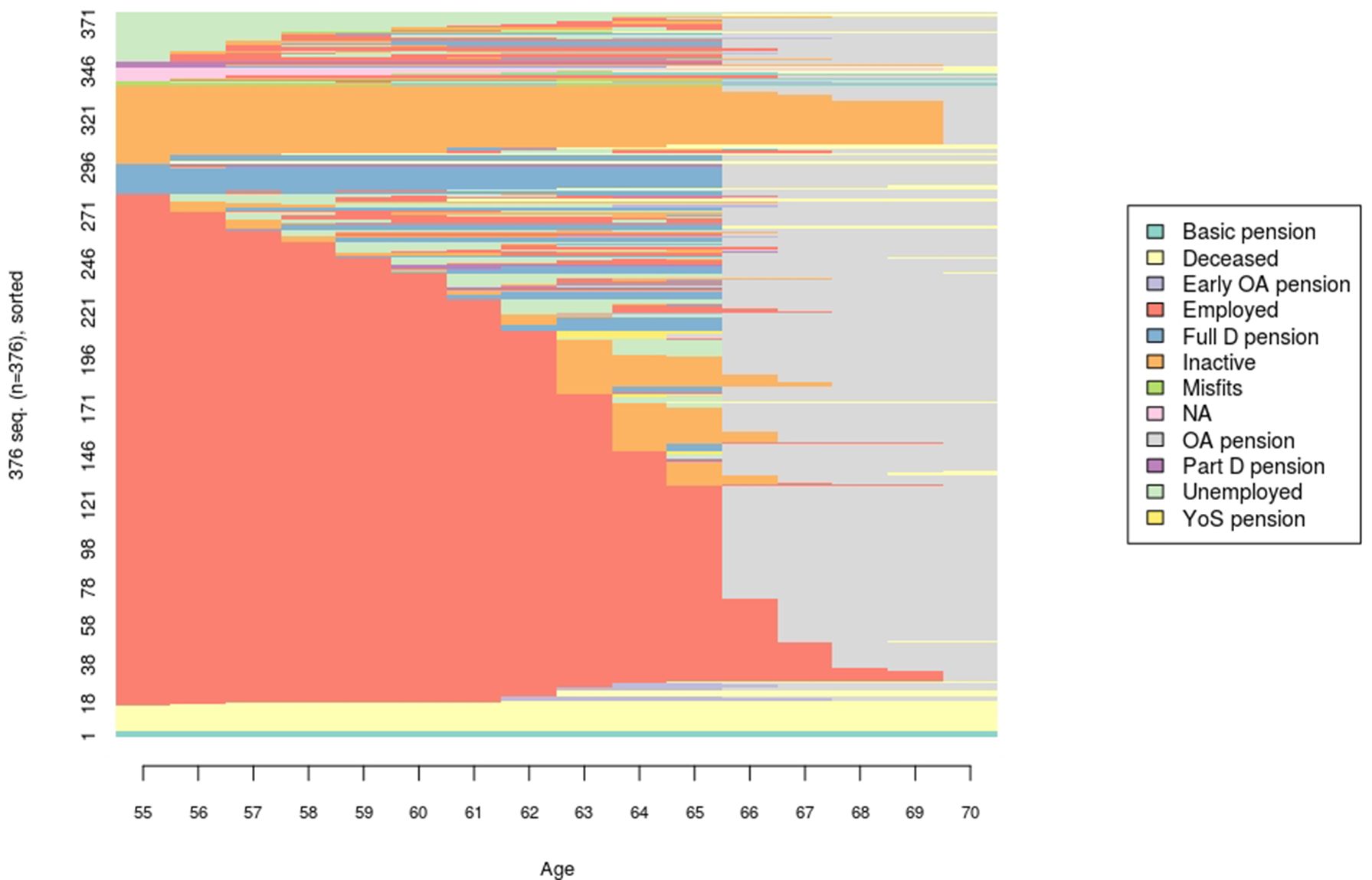
The first analysis shows the individual transitions (the tiny horizontal line in Figure 1). Figure 1 has three dimensions: individual, age and labor market status. The sequence index plot shows every individual as long as the total number of individuals (vertical axis) does not exceed 400. In this example, the number of individuals is 376, for whom the plot visualizes the true transitions from age 55 to 70 (horizontal axis). The individuals are sorted according to their labor market state at age 55. It would also be possible to sort individuals at age 70, which would yield a slightly different, retrospective view of the transition patterns.
Figure 1 shows several things. First, the flexible retirement age for the cohort born in 1970 is 66 years; working is possible until age 69. We see that retirement at the earliest possible age is common, yet we also see some individuals postponing retirement because of positive economic incentives. Second, full employment is the mainstream state at age 55, but after that, there are several possible transition paths. Unemployment, sickness spells and other career breaks become more common before retirement. Retirement on a disability pension also increases after age 55. Along with disability, the share of the deceased increases by age. Finally, Figure 1 also reveals careers ending in unemployment some years before retirement (a persistent feature of the Finnish labor market.
For microsimulation practitioners, Figure 1 provides a quick overview of the actual transitions. It can be used to visually validate model assumptions and parameters. In validating ELSI, the share of the inactives after reaching the retirement age was discussed. However, the proportion is due to the handling of the model population and of the people living outside the country for whom the earnings-related old-age pension is paid at the latest possible age. This is partly a technical assumption and partly an empirical fact, as illustrated by SA.
4.2. Most common transitions
The maximum number of sequences is defined by the number of individuals in a given cohort. The optimal matching technique uses aggregates and joins individuals into typical sequences. For example, the transition sequences of the cohort born in 1970 can be classified into 24 groups with more than two cases in each group. Table 2 shows the five most common sequences and their shares in the sample. The interpretation of the sequences requires clarification. The most frequent sequence (15.4%) for the 1970 cohort is that the individuals (58 cases) are employed for 11 years before retiring on an old-age pension for 5 years, so technically, the sequence is EEEEEEEEEEEOOOOO.
Five most common transition sequences of cohorts born in 1970, 1980, 1990 and 2000, individuals and shares.
| Transition sequence | Count | % |
|---|---|---|
| 1970 | ||
| EMP/11 - oap/5 | 58 | 15.4 |
| INA/15 - oap/1 | 23 | 6.1 |
| EMP/12 - oap/4 | 22 | 5.9 |
| DEC/16 | 13 | 3.5 |
| EMP/13 - oap/3 | 13 | 3.5 |
| 1980 | ||
| EMP/12 - oap/4 | 57 | 15.4 |
| INA/15 - oap/1 | 25 | 6.8 |
| DEC/16 | 16 | 4.3 |
| EMP/13 - oap/3 | 14 | 3.8 |
| fdp/12 - oap/4 | 11 | 3.0 |
| 1990 | ||
| EMP/13 - oap/3 | 71 | 15.5 |
| INA/15 - oap/1 | 35 | 7.6 |
| EMP/14 - oap/2 | 28 | 6.1 |
| EMP/15 - oap/1 | 14 | 3.1 |
| fdp/13 - oap/3 | 13 | 2.8 |
| 2000 | ||
| EMP/13 - oap/3 | 54 | 14.0 |
| INA/15 - oap/1 | 26 | 6.7 |
| EMP/14 - oap/2 | 18 | 4.7 |
| EMP/15 - oap/1 | 18 | 4.7 |
| fdp/13 - oap/3 | 10 | 2.6 |
Table 2 illuminates a number of substantial things. First, a transition from employment into old-age retirement is by far the most common sequence for the selected cohorts. State counts further indicate that the 1970 cohort will retire on an old-age pension at age 66, and subsequent cohorts one to two years later, as it should be according to the assumptions of the ELSI model. Second, the second most common sequence among the selected cohorts collects the inactive-to-old-age pension transitions. Finally, the sequences of later old-age retirement are also becoming more common among younger cohorts.
For microsimulation practitioners, Table 2 offers a more aggregated view of the model transition classes. A good way to validate simulated model transitions would be to look at a broader list of transition sequences of selected cohorts (or other classes) in order to check the shares and, thus, the logic of the model transitions.
4.3. Transition rates
Transition rates between states give numerical estimates of model transitions. Table 3 shows a matrix where each row gives a transition distribution from the associated original state in t to the states in t+1 (the figures add up to one in each row). The alphabets are explained in Table 1.
Transition rates of cohort born in 1970, per cent.
| To | ||||||||||||
|---|---|---|---|---|---|---|---|---|---|---|---|---|
| From | bap | DEC | eop | EMP | fdp | INA | MIS | NA | oap | pdp | UNE | yos |
| bap | 97.0 | 1.5 | 0.0 | 0.0 | 0.0 | 0.0 | 1.5 | 0.0 | 0.0 | 0.0 | 0.0 | 0.0 |
| DEC | 0.0 | 100.0 | 0.0 | 0.0 | 0.0 | 0.0 | 0.0 | 0.0 | 0.0 | 0.0 | 0.0 | 0.0 |
| eop | 0.0 | 0.0 | 72.7 | 0.0 | 0.0 | 0.0 | 0.0 | 0.0 | 27.3 | 0.0 | 0.0 | 0.0 |
| EMP | 0.0 | 0.3 | 0.2 | 87.0 | 0.4 | 4.0 | 0.0 | 0.0 | 5.2 | 0.2 | 2.4 | 0.3 |
| fdp | 0.0 | 1.1 | 0.0 | 0.8 | 82.1 | 0.3 | 0.0 | 0.0 | 15.4 | 0.3 | 0.0 | 0.0 |
| INA | 0.0 | 0.5 | 0.1 | 1.2 | 5.3 | 77.9 | 0.0 | 0.0 | 11.9 | 0.1 | 2.8 | 0.0 |
| MIS | 16.7 | 6.7 | 0.0 | 0.0 | 0.0 | 0.0 | 73.3 | 0.0 | 0.0 | 0.0 | 3.3 | 0.0 |
| NA | 0.0 | 2.6 | 0.0 | 5.1 | 0.0 | 0.0 | 10.3 | 82.1 | 0.0 | 0.0 | 0.0 | 0.0 |
| oap | 0.0 | 0.5 | 0.0 | 0.0 | 0.0 | 0.0 | 0.0 | 0.0 | 99.5 | 0.0 | 0.0 | 0.0 |
| pdp | 0.0 | 0.0 | 0.0 | 0.0 | 4.8 | 2.4 | 0.0 | 0.0 | 16.7 | 76.2 | 0.0 | 0.0 |
| UNE | 0.0 | 0.6 | 1.6 | 14.9 | 0.0 | 6.3 | 0.3 | 0.0 | 10.8 | 0.0 | 65.4 | 0.0 |
| yos | 0.0 | 0.0 | 0.0 | 0.0 | 0.0 | 0.0 | 0.0 | 0.0 | 50.0 | 0.0 | 0.0 | 50.0 |
First, Table 3 implies that transition probabilities within the labor market state (diagonal elements) have values close to one, meaning that an individual in a given state at time t has a great probability to remain in the same state at time t+1. For example, transitions from bap to bap (drawing basic pension) over study ages are highly stable (97.0%), whereas transitions from UNE to UNE (staying unemployed) indicate higher instability (65.4%). The instability of transitions from EMP to EMP (staying employed) is 87.0%, indicating the various risks around the employed. Second, transition probabilities between states are also displayed in Table 3. Although a transition from UNE to UNE is the most likely one, there are also other possible transitions, such as from UNE to EMP (14.9%), from UNE to oap (10.8%) and from UNE to INA (6.3%). The probability of staying employed is high, yet there are notable transition probabilities from EMP to oap (5.2%), from EMP to INA (4.0%) and from EMP to UNE (2.4%).
In validating microsimulation model transitions, similar tables could be useful in comparing simulated cohorts.
4.4. State distribution plot
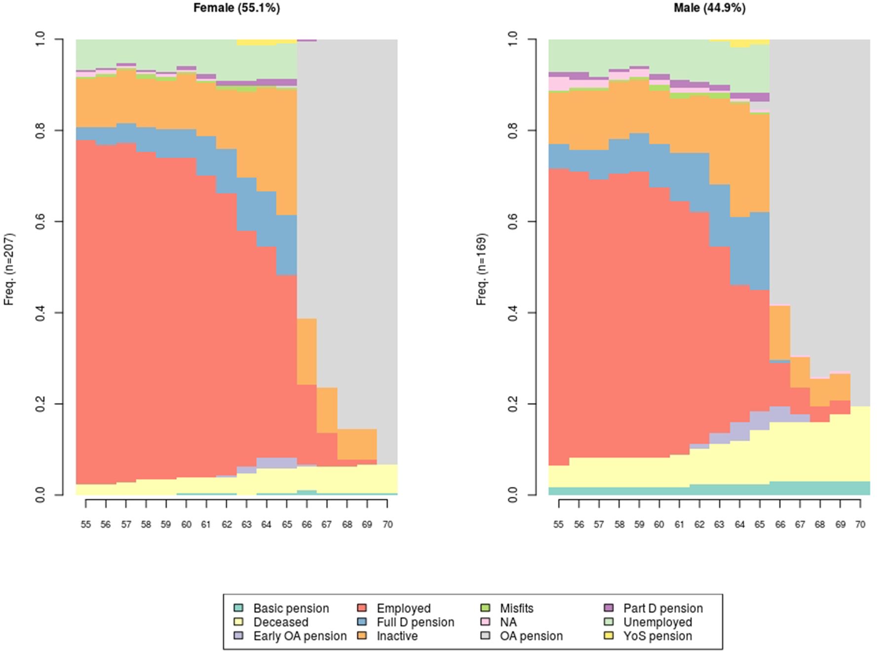
The state distribution plot (or status proportion plot) offers another perspective on model states. The plot can be drawn by any interesting ex ante classification rule to make substantial comparisons within a cohort. Figure 2 show the shares of men (44.9%) and women (55.1%) in the sample. In essence, the plot shows the state distribution, that is, the share of statuses by time points (age). Age is shown on the horizontal axis, whereas the vertical axis is defined by a percentage scale. Figure 2 shows the same cohort and individuals as Figure 1, but by gender. Beside gender, Figure 2 has two additional dimensions: age and labor market status. Here are not clustered and transition sequences are not part of this perspective.

State distribution plot for the 1970 cohort by gender, per cent.
Figure 2 shows that the share of employed at age 55 is relatively high. The share is approximately 80 per cent for women and slightly smaller, about 65 per cent, for men. At age 66 (the retirement age), about 60 per cent of the men and women retire. At age 70, about 80 per cent of the men draw an old-age pension, 16 per cent are deceased and 4 per cent draw a national pension. For women, the shares are different. About 92 per cent draw an old-age pension, 7 per cent are deceased and about one per cent draw a national pension. The gender difference in the mortality assumption is visible here as the share of the deceased is greater already at age 55. Figure 2 also shows the increasing shares of disability pensioners with rising age.
For microsimulation practitioners the state distribution plot offers similar possibilities to validate model transitions as does Appendix table A.3. The share of cases in different model states at a given age can be compared to auxiliary information sources.
4.5. Mean time in state
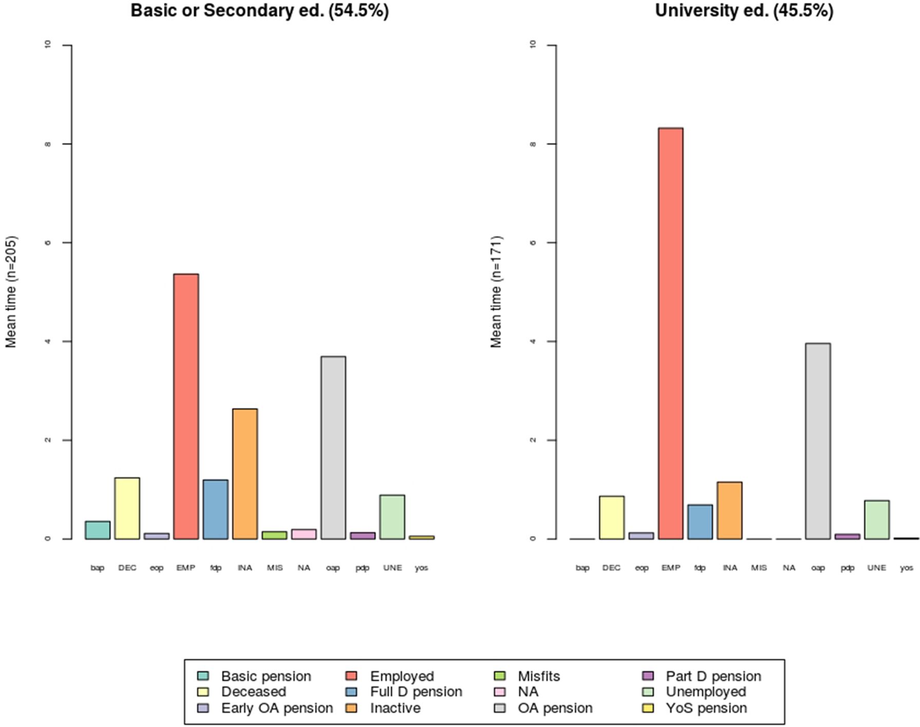
A useful measure in comparing classes such as gender or level of education is the mean time spent in each state. Figure 3 shows the mean estimates by education. The dataset is split by the level of education. One group consists of individuals with at least a secondary education (Basic or Secondary ed.), and another group consists of people with a higher-level education (Low or High univ.). There are slightly more people with a lower-level education (54.5%) than a higher-level education (45.5%).

Mean time in state for 1970 cohort by education, years.
As expected, the employment attachment is stronger among the highly educated who have more than eight years of employed time (EMP). For those with a lower-level education the employed time is under six years. As a result, those with a lower-level education spend more time on a full disability pension (fdp) and as inactive (INA).
4.6. Clustering of the sample
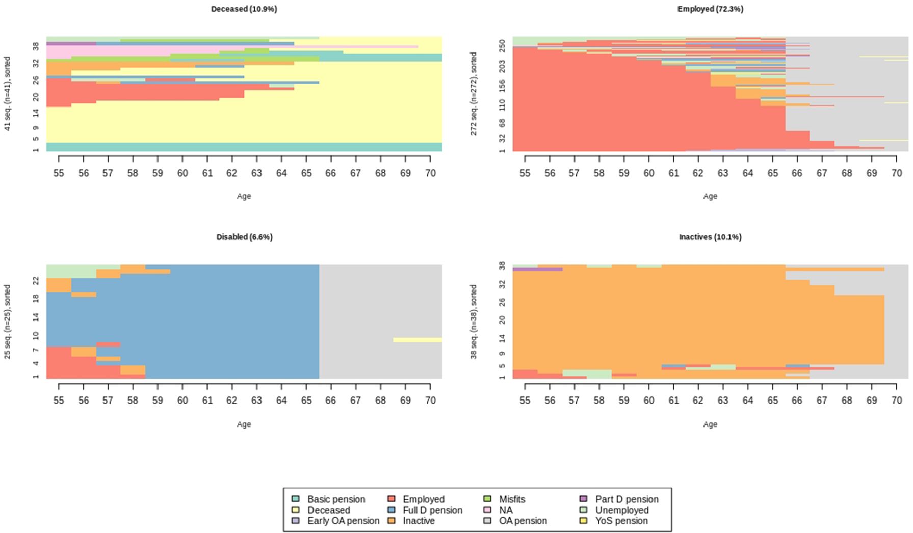
The aforementioned sequence aggregation is preliminary clustering. The sample can be divided into sub-groups. To make a typology of the transition sequences, a Ward hierarchical clustering of the sequences from the optimal matching distances are made and for each individual sequence, the cluster membership of the four-group solution is retrieved. Naturally other groupings are possible, as well as a different number of clusters.
The clustering makes it possible to focus on the possible latent groups within the sample. The clustering could also be useful in illustrating substantial topics. In the following, we have named the clusters heuristically. Figure 4 shows that the largest cluster (Employed 72.3%) consists mainly of those whose employment is strong when approaching retirement. There are two clusters of equals sizes. One consists of the deceased and individuals drawing a basic pension only (Deceased 10.9%) and another of the inactives (Inactives 10.1%). The smallest cluster (Disabled 6.6%) consists of cases with a disability pension before the old-age pension.

Clustering transition sequences of cohort born 1970.
5. Trajectory analysis of employment
Trajectory analysis is a natural statistical reference point for sequence analysis, but what added value does SA provide compared to TA? As was shown in chapter 4, SA is a technique that can illuminate data contents such as model transitions in great detail. On the other hand, TA is commonly used in identifying latent sub-groups in sample and visualizing mean developments in outcome(s). Next, we will show how TA can be used to analyze the same labor market transition data.
5.1. Modeling developmental trajectories
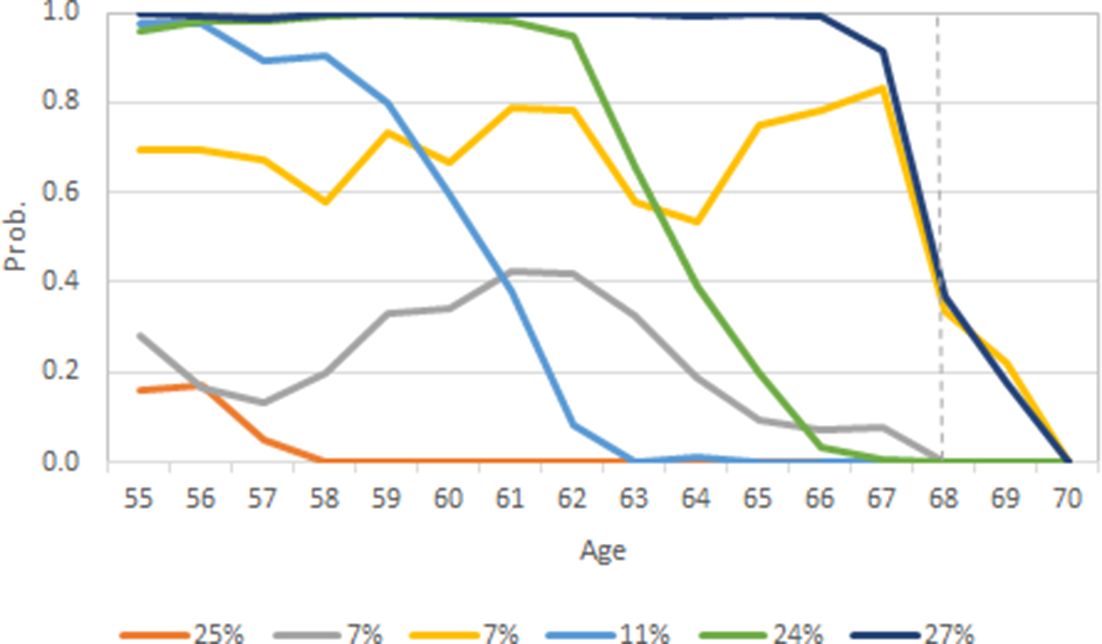
Following the practices in Salonen et al. (2019), a TA was done for analyzing employment near old-age retirement for a cohort born in 2000. Using the example data (findata) and transforming the outcome variable (EMP transformed into binary variable: 1=Employed, 0=Not employed) and independent variables slightly, a univariate TA can be done. Selecting the number of sub-groups using BIC criterion (k=2 to 6: -2316.8, -1980.4, 1888.8, 1832.7 and -1819.2) indicates that a six-group solution yields the best statistical model fit. By subjective evaluation of the solution, the results are reasonable. Figure 5 shows the employment trajectories, that is, the group averages of six sub-groups. We can see that there are two groups with sizes 27% and 7% with relatively high and stable probabilities of employment until old-age retirement. There are also two groups with sizes 11% and 24% with gradually decreasing probability of employment with age. Finally, there are groups with sizes 25% and 7% with persistently low probability of employment.

Employment trajectories of cohort born in 2000 (k=6). Dotted line indicates old-age retirement age.
TA is most useful in this kind of analysis, focusing on one or just a couple of analysis variables. The analysis reveals the latent groups and associated developmental trajectories. It is possible to formulate a multivariate TA (e.g. Nagin et al., 2018; Nummi et al., 2017) to analyze several outcomes simultaneously. However, this kind of analysis was not successful with the available measures. Furthermore, with TA it would be possible to analyze the group composition and even model factors affecting group membership.
In analyzing model transitions, SA gives more detailed information (at individual level) compared to TA. SA also captures a range of model states in the figures (12 in the above examples). SA also provides interesting additional measures, as was shown in chapter 4, which are lacking in TA. If detailed individual-level information is not necessary, TA could be more useful with certain outcomes. For example, focusing on monetary measures, such as wages and pensions, could better be analyzed with TA. In addition to monetary measures, the TA can also be used to illuminate developmental trajectories in nominal variables such as level of education.
6. Conclusion
The results of dynamic microsimulation oftentimes include simulated dataset(s), which entail individual level information about labor market or population transitions over a simulated time-period. For example, the data contents could include labor market patterns related to employment, unemployment, sickness spells or retirement. Population patterns such as level of education, occupation selection, or family configurations are also common elements in dynamic microsimulation. All the information contents of simulation must be modeled sensibly and consciously, yielding credible heterogeneity within the simulated population. In fact, microsimulation is a controlled framework in which to create biographical trajectories.
Sequence analysis (SA) can be an interesting tool for microsimulation practitioners when investigating simulated heterogeneity and revealing possible latent transformation patterns. In a nutshell, SA includes three steps. First, the data is coded, divided into subsets, and formatted for the core program (e.g., R). Second, the sequences are counted and usually compared by means of optimal matching analysis. Finally, typologies of transformation sequences are obtained by clustering analysis. These steps were presented in this study.
This study showed, in detail, how to use SA with simulated data from the Finnish ELSI model. The examples given were based on transitions near retirement. Beside retirement modeling or labor market modeling in general, SA could also be applied with other dynamic models such as firm or farm models as long as the models simulate states in discrete time steps.
There is another statistical technique called trajectory analysis (TA), which can be used together with SA to analyze microsimulation outcomes. SA gives a detailed overview of individual model transitions, whereas TA is applicable in visualizing sub-population mean developmental trajectories. For microsimulation practitioners, the simulated outcomes determine which statistical technique is most useful. Certainly, SA and TA complement each other.
In practice SA can be used to visualize microsimulation results, and to validate simulation. The sequence index plots are a powerful tool in visualizing transition patterns. The model validation can also benefit from visual inspection of sequences, but more from the subsetting and grouping options, which allow for a study of the coherence of simulated groups.
SA did not reveal any serious misspecification in the ELSI model. The labor market transitions in ELSI are driven by ex ante defined transition probabilities. This kind of modeling is sensitive to misspecification. Therefore, a clustering technique like SA is useful in model validation.
This study showed certain possibilities and one practical application of the TraMineR and TraMineRextras packages in a microsimulation context. There are further useful functions, but they are beyond the scope of this study.
A.1 An example R code
The TraMineR and TraMineRextras packages count a number of measures to collate and visualize transition sequences. In this example we show some of their possibilities in microsimulation. The example data (findata.dat) are drawn from the model and consist of simulated individuals of a cohort born in 2000. The data focus on individuals aged 55 to 70.
The TraMineR library needs a distinct color for each microsimulation model state. A color palette is therefore attached to the sequence object. A default color palette is automatically selected according to ten number of model states. The library accepts both numerical and character measurements.
The first step of the analysis is to load the necessary libraries and retrieve the sample data. The sample (n=387) is from the simulated dataset. The view(findata) function gives an overview of the data. The data content is the following: case number, birth-year, education, gender and model statuses (16 longitudinal measurements). The par(mfrow = c(2 2)) function can be used, with different argument values when necessary to divide the graphic area. The arguments used divide the graphical area into two rows and two columns.
Initializing the session.
1. library(TraMineR)
2. library(TraMineRextras)
3. library(cluster)
4. findata <- read.table("findata.dat", header = TRUE, na.strings = "NAS")
5. View(findata)
6. par(mfrow = c(1, 1))
The labor market states are defined as in the actual dataset in function findata.alphabet. The model states are assigned abbreviations and labels in functions findata.labels and findata.scodes, which are user-definable. The abbreviations are a necessity to draw clear and informative figures.
Creating formats and abbreviations.
1. findata.alphabet <- c("Basic pension", "Deceased","Early OA pension","Employed","Full D pension","Inactive","Misfits","NA","OA pension","Part D pension","Unemployed","YoS pension")
2. findata.labels <- c("Basic pension","Deceased","Early OA pension","Employed","Full D pension","Inactive","Misfits","NA","OA pension","Part D pension","Unemployed","YoS pension")
3. findata.scodes <- c("bap","DEC","eop","EMP","fdp","INA","MIS","NA","oap","pdp","UNE","yos")
The data are read to create a state sequence object from the age specific status variables (columns 5 to 20). If there is no need to further subset the sample, the first line of the code is not completely necessary. However, because of some functions (see Algorithm 5), it is practical to subset the sample by, for example, gender or education. The subsets are defined as different sequence objects. The seqlegend(findata.seq) function illustrates the colors attached to the states.
Selecting subsets of sample and analysis variables.
1. findata <- findata[which(findata$Birth_year == 2000),]
2. findata.seq <- seqdef(findata, 5:20, xtstep = 1, alphabet = findata.alphabet, states = findata.scodes, labels = findata.labels)
3. seqlegend(findata.seq)
The next step initializes the actual SA. The individual labor market transition sequences in the sample are drawn by the function seqIplot. The essential argument is sortv, which defines the sorting order for different illustrations. In this example, the observations are sorted by the first model status (at age 55). A slightly different graph can be drawn with the option sortv = "from.end". The rest of the arguments are merely to adjust the graphics.
Labor market transition sequences.
1. seqIplot(findata.seq, sortv = "from.start", cex.lab = 0.8, cex.axis = 0.8, cex.legend = 1.3, with.legend = "right", xlab = "Age", xtstep = 1)
The function seqtab aggregates the transition sequences to some extent. The function prints the most common sequences into the console with frequencies and shares. This function can be used, for example, to compare classes in the sample. However, this would require subsetting the sample according to the interesting classes in Algorithm 3. The number (5) of the most common sequences is given in the argument idxs.
Common transition sequences, five most common.
1. seqtab(findata.seq, format = 'SPS', idxs = 1:5)
Microsimulation practitioners are familiar with transition probabilities between model states. They are counted by the seqtrate function, which prints the transition probabilities from one state to the next ones in the console.
Transition probabilities.
1. tr <- seqtrate(findata.seq)*100
2. round(tr, 1)
The state distributions are calculated in the seqdplot function. This example shows the state distribution by gender, which is defined by the group argument. The rest of the arguments are merely to adjust the graphics.
Labor market state distribution by gender.
1. seqdplot(findata.seq, group = group.p(findata$Gender), cex.main = 0.9, cex.lab = 0.9, cex.axis = 0.9, with.legend = TRUE, border = NA, xlab = "Age", xtstep = 1)
The seqmtplot function provides a useful measure to compare different classes, namely mean time in state. This example shows the mean times by education group (level of education) which, in this function, is also defined by the group argument. The rest of the arguments are merely to adjust the graphics.
Mean time in model state.
1. seqmtplot(findata.seq, group.p(findata$Education), cex.lab = 0.8, cex.axis = 0.6, with.legend = FALSE, xtstep = 1, ylim = c(0, 10))
An essential addition to SA is clustering analysis, which is used to find latent sub-groups in the sample. The next step is to illustrate the clustering. Using OMA, a four-group partition of the sample is obtained with Algorithms 9 and 10. In the first stage, OMA is applied by computing pairwise optimal matching distances between transition sequences, using an insertion or deletion cost of 1, and a substitution cost matrix, which is based on observed transition rates. The Ward method is used in this example.
The second stage of the analysis is HCA. When proceeding to an agglomerative hierarchical clustering using the obtained distance matrix, we select the four-cluster solution and express it as a factor. The number of clusters (k=4) is user-defined. The group-assignment can be retrieved for further analysis via factors in object cl1.4fac, which is used in subsequent steps of SA.
Initializing optimal matching analysis.
1. dist.om <- seqdist(findata.seq, method = "OM", indel = 1, sm = "TRATE")
Initializing cluster analysis.
1. clusterward <- agnes(dist.om, diss = TRUE, method = "ward")
2. cl1.4 <- cutree(clusterward, k = 4)
3. cl1.4fac <- factor(cl1.4, labels = paste("Cluster", 1:4))
The clusters can be further illustrated, for example, by functions seqIplot and seqdplot. Algorithm 11 is similar to 7, with the difference that the grouping is done by the cluster assignments. The rest of the arguments are again merely to adjust the graphics.
Labor market state distribution by cluster.
1. par(mfrow = c(2, 2))
2. seqdplot(findata.seq, group = group.p(cl1.4fac), border = NA, xlab = "Age", cex.main = 0.8, cex.lab = 0.8, cex.axis = 0.8, xtstep = 1)
For further statistical analyzes it can be useful to merge the original dataset and clustering result (see Algorithm 12).
Adding the cluster variable to the dataset
1. findata.seq$cl1.4fac <- cl1.4fac
ELSI model states.
| No. | Contents |
|---|---|
| 15 | Full-time employed for the first consecutive year |
| 16 | Full-time employed for the second consecutive year |
| 1 | Full-time employed for at least the third consecutive year |
| 2 | Unemployed (excluding those on an unemployment pathway to retirement) |
| 3 | On an unemployment pathway to retirement |
| 4 | Sickness benefits preceding full disability pension |
| 5 | Part-time pension |
| 11 | Partial old-age pension and employed |
| 10 | Partial disability pension and employed |
| 6 | Years-of-service pension |
| 7 | Partial old-age pension and not employed |
| 8 | Old-age pension |
| 17 | Full disability pension for the first consecutive year |
| 9 | Full disability pension for at least the second consecutive year |
| 18 | Partial disability pension and not employed |
| 21 | National old-age pension only |
| 22 | National disability pension only |
| 13 | Outside the labor force but has accrued earnings-related pension |
| 19 | Permanently outside the labor force but has accrued earnings-related pension |
| 20 | Outside the labor force and has not accrued earnings-related pension |
| 12 | Deceased |
Labor market states of the cohort born in 1970 at ages 55 to 70, per cent.
| Labor market state | 55 | 56 | 57 | 58 | 59 | 60 | 61 | 62 | 63 | 64 | 65 | 66 | 67 | 68 | 69 | 70 |
|---|---|---|---|---|---|---|---|---|---|---|---|---|---|---|---|---|
| Basic pension | 1 | 1 | 1 | 1 | 1 | 1 | 1 | 1 | 1 | 1 | 1 | 1 | 2 | 2 | 2 | 2 |
| Deceased | 3 | 3 | 4 | 4 | 4 | 5 | 5 | 6 | 6 | 7 | 7 | 8 | 9 | 9 | 10 | 11 |
| Early OA pension | 0 | 0 | 0 | 0 | 0 | 0 | 0 | 0 | 2 | 3 | 3 | 2 | 1 | 0 | 0 | 0 |
| Employed | 69 | 67 | 67 | 65 | 64 | 61 | 59 | 56 | 44 | 37 | 35 | 14 | 5 | 2 | 1 | 0 |
| Full D pension | 5 | 5 | 6 | 6 | 7 | 8 | 10 | 11 | 13 | 15 | 15 | 0 | 0 | 0 | 0 | 0 |
| Inactive | 12 | 12 | 12 | 12 | 12 | 12 | 13 | 13 | 21 | 24 | 24 | 13 | 8 | 5 | 5 | 0 |
| Misfits | 1 | 1 | 1 | 1 | 1 | 1 | 1 | 1 | 1 | 1 | 1 | 0 | 0 | 0 | 0 | 0 |
| NA | 2 | 2 | 2 | 2 | 2 | 2 | 1 | 1 | 1 | 1 | 1 | 1 | 1 | 1 | 0 | 0 |
| OA pension | 0 | 0 | 0 | 0 | 0 | 0 | 0 | 0 | 0 | 0 | 1 | 61 | 75 | 81 | 82 | 87 |
| Part D pension | 0 | 0 | 0 | 1 | 1 | 1 | 1 | 1 | 1 | 1 | 1 | 0 | 0 | 0 | 0 | 0 |
| Unemployed | 8 | 8 | 8 | 8 | 8 | 9 | 10 | 10 | 10 | 10 | 10 | 0 | 0 | 0 | 0 | 0 |
| YoS pension | 0 | 0 | 0 | 0 | 0 | 0 | 0 | 0 | 0 | 1 | 1 | 0 | 0 | 0 | 0 | 0 |
| Total | 100 | 100 | 100 | 100 | 100 | 100 | 100 | 100 | 100 | 100 | 100 | 100 | 100 | 100 | 100 | 100 |
References
-
1
Sequences of social events: Concepts and methods for the analysis of order in social processesHistorical Methods: A Journal of Quantitative and Interdisciplinary History 16:129–147.https://doi.org/10.1080/01615440.1983.10594107
-
2
Event sequence and event duration: Colligation and measurementHistorical Methods: A Journal of Quantitative and Interdisciplinary History 17:192–204.https://doi.org/10.1080/01615440.1984.10594134
-
3
Optimal matching methods for historical sequencesJournal of Interdisciplinary History 16:471–494.https://doi.org/10.2307/204500
-
4
Sequence analysis and optimal matching methods in sociology: Review and prospectSociological Methods & Research 29:3–33.
-
5
Classifying life course trajectories: A comparison of latent class and sequence analysisJournal of the Royal Statistical Society: Series C 61:765–784.https://doi.org/10.1111/j.1467-9876.2012.01047.x
-
6
Sequence analysis and related approaches innovative methods and applicationsGraphical representation of transition and sequences, In:, Sequence analysis and related approaches innovative methods and applications, Life Course Research and Social Policies 10, Springer.
-
7
New developments in sequence analysisSociological Methods & Research 38:359–364.https://doi.org/10.1177/0049124110363371
-
8
Sequence analysis with StataThe Stata Journal: Promoting communications on statistics and Stata 6:435–460.https://doi.org/10.1177/1536867X0600600401
- 9
-
10
Sequence analysis and related approaches innovative methods and applicationsDo different approaches in population science lead to divergent or convergent models?, In:, Sequence analysis and related approaches innovative methods and applications, Life Course Research and Social Policies 10, Springer.
-
11
Applications of microsimulation modellingProspective microsimulation of pensions in European Member States, In:, Applications of microsimulation modelling, Hungary, Társadalombiztosítási Könyvtár.
- 12
- 13
-
14
Analyzing and visualizing state sequences in R with TraMineRJournal of statistical software 404:1–37.
-
15
SADI: sequence analysis tools for StataDepartment of sociology working paper series WP2014-03, University of Limerick.
-
16
Binary codes capable of correcting deletions, insertions, and reversalsSoviet Physics Doklady 10:707–710.
-
17
But what have you done for us lately? Commentary on Abbott and TsaySociological Methods & Research 291:34–40.
-
18
Detailed molecular model for transfer ribonucleic acidNature 224:759–763.https://doi.org/10.1038/224759a0
-
19
Longitudinal methods for life course research: a comparison of sequence analysis, latent class growth models, and multi-state event history models for studying partnership transitionsLongitudinal and Life Course Studies 8:191–208.https://doi.org/10.14301/llcs.v8i2.415
- 20
-
21
Group-based multi-trajectory modelingStatistical Methods in Medical Research 27:2015–2023.https://doi.org/10.1177/0962280216673085
-
22
New advances in statistics and data scienceStatistical analysis of labor market integration: A mixture regression approach, In:, New advances in statistics and data science, Springer, ICSA Book Series in Statistics.
-
23
Holistic analysis of the life course: methodological challenges and new perspectivesAdvances in Life Course Research 41:100251.https://doi.org/10.1016/j.alcr.2018.10.004
-
24
Extended working lives and late-career destabilisation: a longitudinal study of Finnish register dataAdvances in Life Course Research 35:114–125.https://doi.org/10.1016/j.alcr.2018.01.007
-
25
Sequence analysis and related approaches innovative methods and applicationsSequence analysis: Where are we, where are we going?, In:, Sequence analysis and related approaches innovative methods and applications, Life Course Research and Social Policies 10, Springer.
- 26
-
27
Using trajectory analysis to test and illustrate microsimulation outcomesInternational Journal of Microsimulation 12:3–17.https://doi.org/10.34196/ijm.00198
- 28
-
29
ELSI: The Finnish pension microsimulation modelFinnish Centre for Pensions, Reports 08/2020., http://urn.fi/URN:ISBN:978-951-691-312-7.
- 30
- 31
-
32
Distributional effects of forthcoming Finnish pension reform – a dynamic Microsimulation approachInternational Journal of Microsimulation 83:75–98.
-
33
Hierarchical grouping to optimize an objective functionJournal of the American Statistical Association 58:236–244.https://doi.org/10.1080/01621459.1963.10500845
-
34
Some comments on “Sequence analysis and optimal matching methods in sociology: Review and prospect”Sociological methods & research 29:41–64.https://doi.org/10.1177/0049124100029001003
Article and author information
Author details
Funding
No specific funding for this article is reported.
Acknowledgements
The authors wish to thank chief editor Matteo Richiardi for his many thoughtful comments that greatly improved this article.
Publication history
- Version of Record published: August 31, 2020 (version 1)
Copyright
© 2020, Salonen, Möttönen, TikanmäkiNummi
This article is distributed under the terms of the Creative Commons Attribution License, which permits unrestricted use and redistribution provided that the original author and source are credited.