In-work Benefits in Belgium: Effects on Labour Supply and Welfare
Abstract
Belgium has implemented, following the example of other countries, in-work benefit policies since the early 2000’s, with the objective of increasing employment rates and fighting poverty. Belgian in-work benefits differ from most other in-work benefits as eligibility requires low hourly earnings. We study the effects extensions of those benefits would have both on labour supply and welfare, using a random-utility - random-opportunity model estimated on cross-sectional SILC datasets. Results show that further increasing the benefits would slightly increase labour supply and welfare of low-to-middle income deciles, but at very high net cost per job created. We compare our results with existing research and explain some mechanisms that possibly led to an underestimation of negative intensive margin labour supply responses in previous simulations.
1. Introduction
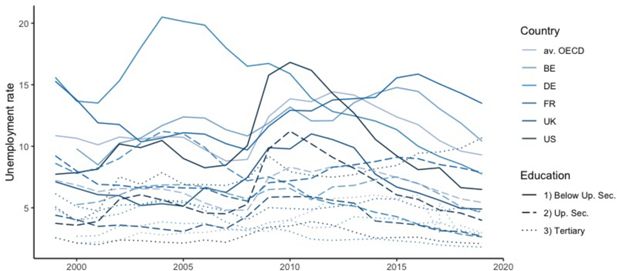
Persistent high unemployment rates, especially for low-skilled workers (see Figure 1), have an important impact on the government budgets, by on one hand lowering the tax revenues and social security contributions, and on the other hand increasing social security expenses as unemployment and social assistance benefits. An important public policy question is therefore if and how those high rates could best be reduced by means of adequate active labour market policies.
Active labour market policies are, in their broad definition, government programmes that intervene in the labour market to help the unemployed find work. They can be divided in five categories: coaching and controlling unemployed in their job searches, training schemes that aim at reducing potential qualification mismatches, flexibilization of labour regulations,1 direct creation of public jobs and tax-benefit reforms that consist of rendering hiring more affordable for employers and working more attractive for unemployed. Measures of this last category typically consist of diminishing labour income taxes and social contributions (or increasing subsidies).2 When those measures are specifically designed with the purpose of providing an income supplement to those that work, they are called ‘‘in-work benefits’’ (IWB). IWB are usually presented by policy-makers as a financial boost for workers by ‘‘making work pay’’ that has the advantages to reduce unemployment traps and to create large compensatory cost effects due to the increase in employment rates.3 By targeting disadvantaged groups on the labour market, IWB also often have the attractive feature of redistributing income, and seem to therefore combine both equity and efficiency improvements.
Two main paths can be taken regarding eligibility to IWB: using labour income (at individual or household level) in the eligibility test, or using hourly labour income in the eligibility test.4 Most in-work benefits (see section 2), are designed according to the first approach. The French ‘‘Prime pour l’Emploi’’ (PPE) and the Belgian ‘‘work-bonus’’ (WB) are examples of the second approach. While both approaches increase the attractiveness of working situations relative to being unemployed or inactive, they have different consequences on the net wages of working options. The first approach creates part-time traps, which is a situation in which a worker has an incentive to work less in order to become eligible to an earnings-tested benefit, or seen differently, a situation where a part-time worker has little incentive to work more due to the phase-out of IWB. To some extent, the scheme also creates low-wage traps, which is a situation where an increase in gross wage will be passed through only to a limited extent to the net wage due to the phase-out of the IWB. This makes it expensive for an employer to increase the net wage of an employee, and reduces the relative attractiveness of higher-paid jobs, giving distorted market-signals to workers. The second approach aims at shifting the reward from low-earning to hard-working but low-earning capacity individuals, by linking the benefit level to hours of labour supplied and restricting eligibility to low hourly wages. This reduces the part-time trap but worsens the low-wage trap, and thus represents a different choice of trade-off between the indirect effect of incentivizing part-time work vs. low-paid work. Besides this dimension, IWB can vary with respect to eligibility thresholds, tapering mechanisms, duration, etc.
Our purpose is to study the effects of in-work benefits targeting individuals having a low hourly wage. For this, we run a partial equilibrium analysis by simulating 3 hypothetical reforms that increase the generosity of the Belgian WB and analyzing resulting effects on employment, using a random-utility random-opportunity model estimated on SILC data. Besides complementing existing research and providing a useful benchmark for countries with similar economies considering such benefits, we shed light on model assumptions of previous simulations that possibly led to an underestimation of the negative labour supply reactions and budgetary costs of such schemes. Moreover, our model uses cross-sectional datasets of different years, which allows to use policy variations over time to improve the identification of the model. Lastly, our study includes a welfare analysis, essential for a thorough policy evaluation.
The paper is structured as follows: Section 2 discusses briefly past research on in-work benefits, and gives an overview of the roll-out of those kind of policies in Belgium. Section 3 details the current Belgian WB scheme. Section 4 presents the labour market model that is used to simulate the reforms. Section 5 presents and discusses the effects of our different reforms on labour supply and income distribution. Results are then compared with previous research. Section 6 concludes.
2. State of research
2.1. International examples of in-work benefits
The most famous and researched examples of in-work benefits are the US Earned Income Tax Credit (EITC) and the UK Working Tax Credit (WTC). Besides those two schemes, we also give some attention to the French PPE, which shares the feature of the Belgian WB of targeting benefits to individuals having low hourly earnings. Other IWB that received significant attention from academic researchers are the German Mini-jobs reform in 2003 and the Self-Sufficiency Project experiment in Canada in the 90’s. A detailed overview of IWB policies in OECD countries and a summary of research findings are available in Immervoll and Pearson (2009).
EITC The EITC, enacted in 1975 and still lasting, is a refundable tax credit for low- to moderate-income working individuals and couples. In this scheme, the amount of the benefit depends on a recipient’s earned income and number of children. Most studies indicate that the scheme has a positive effect on the labour force participation of single mothers (Crandall-Hollick, 2016).5 Regarding the impact on married secondary earners’ decisions to start working, research still is inconclusive. Looking at the intensive margin, most of the empirical evidence indicates the EITC has had a negligible to small effect on the number of hours unmarried people worked, while it has had a negative effect on the hours worked by secondary earners. Lastly, as the EITC was not primarily focused on childless adults, their opportunity sets are less affected and little information has been published regarding potential effects on their labour supply decisions.
WTC The ancestor of the current WTC was introduced in Britain in 1970, under the name Family Income Support.6 The WTC is similar to the EITC but is more generous and is based on net (rather than gross) family income. It has been shown consistently (see Brewer et al. (2006) for a discussion) across a number of studies that the scheme increased participation of single parents significantly. Moreover, it has been estimated that WFTC reduced labour supply of married women, both at the intensive and extensive margin, but that this was more than compensated by labour supply increases among married men.
PPE The PPE was introduced in 2001, reformed a couple of times in the later years, and lasted until 2015, where it was merged with an other IWB, the ‘‘RSA activité’’, into the ‘‘Prime d’activité’’. It’s value is lower than the EITC and WFTC schemes, culminating at a few hundreds of EUR per year. Eligibility is based on full-time equivalent earnings. The benefit also depends on the family situation, and the scaling with respect to working time is not linear, so that the scheme still creates a part-time premium. Almost all studies (see Sterdyniak (2007) and Arnaud et al. (2008) for a detailed overview) find positive but very small employment effects of less than 0.5 percentage points. Stancanelli (2008) even suggests employment losses among married women and no significant gains for non-married women.
2.2. In work benefits in Belgium
2.2.1. History of in-work benefits
The first in-work benefits were deployed at the turn of the century, with the goal of reducing structural unemployment. They were introduced on the one hand through a reduction of social security contributions in December 1999,7 and on the other hand through a refundable earned income tax credit, gradually phased in and phased out and conditional on working at least 13 hours a week, in the summer of 2001.8 Both reforms were intended for low-wage earners. In 2005, those two policies were abolished and replaced by the WB, an extended social security contribution reduction for low-wage earners. The main reason was that the WB, by depending on full-time equivalent labour income instead of actual labour income, avoided part-time traps. Also, the WB had an immediate effect on monthly net earnings, while the tax credit was only computed after the fiscal year: by moving towards an extended WB, the policy maker aimed to render the link between working and the benefit more obvious, to increase the perception of work incentives.
In 2007, using fiscal freedom gained in 2001 in the Lambermont agreements, the Flemish region introduced the ‘‘jobkorting’’ (JK).9 The JK gives a tax credit to those people who earn more than 5500 EUR/year, that phases out between 21.000 EUR/year and 22.250 EUR/year. As it was the case for the first federal income tax credit, eligibility to the JK scheme depended on actual earnings. In 2011 however, for budgetary reasons and after a threat from the European Commission to start a procedure against the measure at the European Court for discrimination,10 the measure was abolished.
In 2011, the WB was complemented with a ‘‘fiscal work-bonus’’ (FWB) that reduces the personal income tax for those eligible to the WB, to further reduce unemployment traps. The level of the FWB is a fixed rate of the WB. In 2015, the government increased the WB and FWB schemes further as part of a broader tax-shift aiming at reducing the tax burden on labour.11
In September 2019, the Flemish government announced the introduction of a large in-work benefit scheme the “Jobbonus” (JB). According to the Flemish government, the policy will be one of the main measures to get 120,000 more people at work in Flanders. At the time of writing, the exact parameters are not known, but the government gives the number of 50 EUR extra net monthly income for low-wage earners, and a complete phase-out at a gross monthly wage of 2500 EUR. They estimated the budget for the measure to be around 350 million EUR yearly.
2.2.2. Research findings
As explained in the introduction, Belgian in-work benefits are quite innovative in the sense that they depend on the full-time equivalent gross labour income and not on the actual labour income, which is supposed to create less negative labour supply incentives at the intensive margin of the labour market. Orsini (2006a) and Dagsvik et al. (2011) discuss this particular feature more in detail and analyze for the first time rigorously the effects of the Belgian WB. They use a discrete-choice labour supply model and compare the policy with some alternative situations, including the tax credit on low earnings that was temporarily implemented in 2001-2004. They conclude that both measures have a positive impact on labour supply but that the WB is more efficient as it avoids the ‘‘part-time trap’’ created by the tax credit system.
Decoster and Vanleenhove (2012) analyze the Flemish Jobkorting (JK). The authors compare the JK with 2 alternative scenarios of JK and show that in all three types of tax credits, labour supply reactions are negative at the intensive margin, and positive at the extensive margin, with a slightly positive net effect. However, the compensatory effects (specifically tax and social security contributions increases due to increases in labour supply) are small and the costs of the measure therefore important.
Vandelannoote and Verbist (2016) analyze various types of hypothetical in-work benefits, playing with income thresholds, tapering mechanisms, individual or household schemes, etc., to give an overview of how the design of the scheme can lead to different effects on poverty and employment.12 They conclude that such benefits imply a trade-off between poverty reduction and labour market activation which has to be considered in light of the aim of the policy. Regarding labour market activation, individual schemes with an income threshold and a tapering-in mechanism seem to work the best, while household schemes perform the best when looking at poverty reduction.
Regarding the future Flemish Jobbonus, Decoster and Vanheukelom (2019) question to what extent those benefits will be effective in increasing labour supply, given already existing federal in-work benefits, and underline the risk of low-wage traps due to high effective marginal tax rates for low-wage earners. Moreover, they show that the purchasing power gains are spread over the income distribution and not concentrated at low disposable income households. Finally, they estimate the cost of the measure at 174 million EUR, quite less than what the Flemish government announced.
3. The Work-Bonus: policy details
The WB is a Belgian in-work benefit that consists of a reduction of social security contributions for individuals with low earning capacity. The level of the WB depends on the full-time equivalent (hereafter FTE) gross salary, denoted , of the employee: for FTE gross salaries lower than a certain threshold , the WB is equal to a fixed amount weighted by the work regime, calculated as where L is the number of hours worked and corresponds to a full-time regime. For FTE gross salaries higher than the fixed amount is tapered out at a rate of , until it reaches at . As explained in subsection 2.2.1., the WB is complemented with a fiscal work-bonus. The fiscal work-bonus is a tax reduction that is calculated as a percentage of the WB. The WB and FWB granted can thus be written:
The values for the above-mentioned parameters for white-collar workers for the year 2016 are given in Table 1.13 Note that the WB cannot exceed social security contributions, and that the fiscal bonus cannot a exceed a maximum value (set at 640 EUR/year in 2016).
Policy parameters (2016): Work-Bonus and Fiscal Work-Bonus
| Parameter | Unit | Value |
|---|---|---|
| A | EUR/month | 193.79 |
| θ 1 | EUR/month | 1,577.89 |
| θ2 | EUR/month | 2,461.27 |
| ρ 1 | % | 21.94 |
| ρ 2 | % | 28.03 |
4. Model
To model workers’ labour supply decisions, we estimate a random utilty-random opportunity (RURO) model, where labour supply is seen as the outcome of agents choosing from a set of job offers. Our model builds on Capéau et al. (2016). For a detailed derivation of the RURO model, see also Dagsvik and Strøm (1992).
We first discuss the database we use and filtering we do in subsection 4.1. Then we go through the building blocks of the model in subsections 4.2. and 4.3.: the utility functions and the opportunity functions. In section 4.4. we calculate the probability that an individual chooses a job with a given wage and amount of required hours. Having the actual worked hours in the database, we can compute the parameters of the utility and opportunity functions that maximize the likelihood that the sample was observed. This procedure is explained in section 4.4..
4.1. Data
To estimate our model, we use the Belgian database of the European Union Statistics on Income and Living Conditions (EU-SILC). This database is representative for the Belgian population and contains information on income, socio-demographic situation and various other dimensions related to labour supply. We assume preferences of individuals did not change over the time of the different EU-SILC surveys used (2006-2017) in our estimation.14 If preferences did indeed not change significantly over time, our method would increase the accuracy of the estimates on one hand because there are more observations, and on the other hand because people are observed in different tax-benefit contexts, helping for the identification of preferences. The tax-benefits system of the corresponding years are used to calculate the disposable incomes (section 4.3.), which are up-rated with consumer price indices to render them comparable.
We consider two types of households: singles workers (hereafter: singles) and couples of workers (hereafter: couples). Singles are defined as households with one adult person that is available to the labour market (i.e. aged between 16 and 64 years and not being sick, in education, disabled or (pre-)retired). Couples are households with 2 adult people that are available to the labour market, and those 2 people form a couple. All other types of households are dropped as their labour supply decision processes might differ too much from the typical cases (e.g. households with one parent and one child available to the labour market are excluded). We also exclude people declaring outlying (>70 h/week) numbers of weekly worked hours, and outlying wages (>60 EUR/h), as well as self-employed for whom information on labour income and worked hours might be less reliable. The percentage of labour market available individuals included in our sample varies from 64.9 to 69.4 , depending on the survey year. Descriptive statistics of the selected households are given in Table 2.
Descriptive statistics - households included in the estimation sample
| Single | Couple | |||
|---|---|---|---|---|
| Male | Female | Male | Female | |
| Number of observations | 4057 | 4585 | 8344 | |
| Av. working time - Workers (h/week) | 39.6 | 34.9 | 40.7 | 32.9 |
| Average hourly gross wage (EUR/h) | 20.3 | 19.9 | 22.2 | 19.7 |
| Participation (%) | 77.3 | 74.7 | 96.1 | 92.6 |
| Highest level of education (%) - Workers | ||||
| - Primary or no education | 6.1 | 5.2 | 4.4 | 3.8 |
| - Lower secondary education | 13.3 | 10.7 | 11.0 | 8.0 |
| - Upper secondary education | 37.2 | 31.4 | 36.0 | 30.2 |
| - High education | 43.5 | 52.8 | 48.6 | 57.9 |
| Highest level of education (%) - Non-workers | ||||
| - Primary or no education | 24.1 | 25.3 | 22.5 | 14.8 |
| - Lower secondary education | 28.4 | 23.1 | 22.2 | 24.7 |
| - Upper secondary education | 27.8 | 33.2 | 36.4 | 35.6 |
| - High education | 19.7 | 18.5 | 18.8 | 25.0 |
| Household composition | ||||
| Average household size | 1.4 | 1.8 | 3.3 | |
| - of which children | 0.1 | 0.6 | 1.3 | |
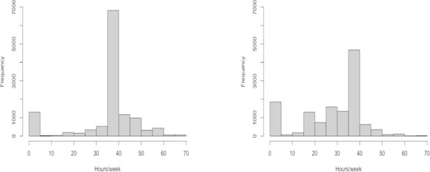
An histogram of the hours worked, by gender, is displayed in Figure 2. The hours worked are those declared by the surveyed individuals, when asked how much hours per week they work on average (including overtime) in their main and complementary jobs. It is important to note that in our sample, overtime workers (that we define as workers working more than 40 hours per week, as will be explained in 4.3.) represent 19% of the population. This is substantially more than what is observed in administrative data, where overtime hours are due to people combining different jobs and represent less than 2% of situations.15 While self-reported data is known to be vulnerable to exaggeration or biases,16 we believe that this discrepancy reveals that many workers work more than contractual (or legal) hours, what may lead to different estimations of hourly wages, that are computed as gross earnings divided by worked hours. Our assumption is that people working more than contractual hours are generally compensated by a higher wage (in other words, they accept a job that is expected to necessitate frequent overtime, if this job provides a consequential salary). This assumption seems supported by the fact that people working overtime declare higher monthly earnings. In this regard, using survey data might bring an insightful and more accurate estimation of hourly wages, especially when used as a proxy for earning capacity. Moreover, as tax-benefit reforms might alter the relative attractiveness of such over-time opportunities (see sub-section 5.2.), including them more accurately in the opportunity sets of individuals will provide a more complete picture of likely behavioural changes. The profiles of those overtime workers are detailed in Table 3.
Descriptive statistics - overtime workers in sub-sample
| Work regime | Comparison | ||
|---|---|---|---|
| All | Overtime | ||
| (>0h/w) | (>40h/w) | ||
| Average age | 40.4 | 40.4 | +0 |
| Average working time (h/week) | 37.1 | 49.5 | +12.4 |
| Average years of education | 13.3 | 14.4 | +1.1 |
| Average gross hourly wage (EUR 2016) | 20.7 | 21.5 | +0.8 |
| Average gross earnings (EUR 2016) | 3310.5 | 4569.7 | +1259.2 |
| Percentage of males | 51.9 | 72.6 | +20.7 |
| Type of ISCO occupation (%) | |||
| - 0: Armed forces | 0.7 | 0.5 | -0.2 |
| - 1: Senior officials and managers | 6.5 | 18.2 | +11.7 |
| - 2: Professionals | 23.5 | 32.2 | +8.7 |
| - 3: Technicians | 16.0 | 15.0 | -1.0 |
| - 4: Clerical support workers | 19.3 | 11.9 | -7.4 |
| - 5: Services and sales workers | 9.9 | 6.7 | -3.2 |
| - 6: Skilled agricultural | 0.4 | 0.3 | -0.1 |
| - 7: Craft and trade workers | 8.5 | 6.4 | -2.1 |
| - 8: Plant and machine operators | 6.0 | 5.9 | -0.1 |
| - 9: Elementary occupations | 9.2 | 2.8 | -6.4 |
4.2. Utility
Let denote the utility of an individual i choosing a job j, and denote the utility function of couple i choosing jobs and , where is the disposable income, the weekly hours of leisure (equal to time endowment minus the number of working hours required for the job opportunity) and a taste shifter corresponding to the job choice(s). Superscripts m (male) and f (female) represent the respective variables of the members of a couple. The utility function is assumed to be decomposable into a deterministic function and the random taste shifter that represents utility derived from unobserved (by the researcher) attributes of a job. This taste shifter is assumed to be i.i.d. distributed across job combinations and households according to a Gumbel distribution with location parameter and scale parameter .
The deterministic part of the utility function is assumed to have the following Box-Cox structural specification17 for singles (Equation 3), where the parameters are allowed to differ for single males and single females, and couples (Equation 4), for which a cross-leisure term is added:
We allow for heterogeneity in the marginal rates of substitution between leisure and income by introducing covariates related to age, number of children in different age-categories, region and education linearly into the leisure parameters ( , , ):
where X are vectors of covariates.
4.3. Opportunities
We assume hourly wages are drawn from a log-normal distribution and are independent of hours worked.
where and the vector γ are parameters. is a vector of covariates that might affect the median of the wage distribution: education, gender, (potential) experience and survey year.
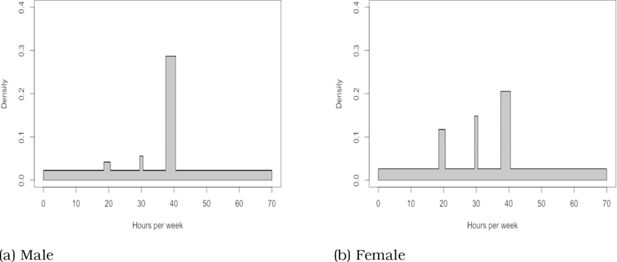
Average weekly working hours of job opportunities are assumed to be drawn from a uniform-with-peaks distribution, where the peaks are chosen to correspond to typical part-time regimes as well as the full-time regime, and where parameters allow to calibrate their height. Peak height can differ only by gender, reflecting the fact that part-time jobs are mostly available in female-dominated sectors of activity (Meulders and O’Dorchai, 2009): health and social work, other community, social and personal service activities, private households with employed persons and also, although to a lesser extent, education. The domain represents the possible values, and is assumed to range from to .
In addition, a number of ‘‘out-of-market’’ job opportunities can be available to the individuals. The intensity of job offers relative to out-of-market opportunities is allowed to vary across individuals, according to the gender and a set of covariates.
where is the vector of covariates that includes region, education level and group-specific unemployment rate. The group-specific unemployment rate corresponds to the unemployment rate per gender-education group, taken from Eurostat. Those rates vary across years and are assumed to be inversely related to the number of suitable jobs accessible to those groups of individuals at a particular point in time. The inclusion of this variable therefore could improve the identification of job-offer intensities.
For each job opportunity requiring an amount of hours h, the gross wage is computed as the multiplication of required hours h and the hourly wage w. EUROMOD then allows to calculate the disposable income corresponding to the job choice: it takes gross income values as an input and determines,18 based on the socio-demographic characteristics of the households, the amount of taxes and benefits they are subject and eligible to, which are respectively subtracted and added to the gross income. This transformation is denoted .
We assume that people opting for an out-of-market opportunity apply for means-tested social assistance. In practice, people not working are eligible to unemployment benefits under the condition that they have a sufficient work-history and are involuntarily unemployed. When, on the contrary, an employee voluntarily quits his job, he can be subject to a penalty of some weeks (from 4 to 52) before being eligible to unemployment benefits. If the employee leaves his job with the intention of relying on unemployment benefits on the long run, he can even be sanctioned indefinitely. Those not eligible to unemployment benefits can apply for social assistance. In that case a thorough means-test, encompassing also means of relatives and assets owned, can be expected. Those being ineligible or not applying to those two schemes (due to stigmatization for example) probably rely on some types of private transfers, personal savings, informal work, mendicancy, etc., as basic needs have to be fulfilled. It is difficult to infer from the data in which of those situations workers opting for an out-of-market opportunity would end up, due to limited information on their preferences and financial situation. For those that are observed not working the same assumption is made, even tough some report unemployment benefits. The reason is that it would be difficult to consider those benefits, that are observed at one point in time, as representative of the level of revenue those individuals (expected to) receive when not working, as such benefits decrease importantly over time.
Considering means-tested social assistance benefits as the out-of-labour income is therefore a simplification needed to compensate the lack of information and an approximation of a consumption floor for survival. An additional argument could be that, especially since the reform of 2012,19 the declining unemployment benefits come near (and even drop below, for cohabitants) social assistance benefit levels in the long-term (see Galand and Termote, 2014), and that our assumption thus does not misrepresent too much the evaluation of out-of-market opportunities by forward-looking agents with reasonably low discount rates counting on unemployment benefits.
4.4. Probability and MLL estimation
Let’s define . The likelihood that an individual i will choose a particular job offer requiring labour time , and paying a wage w, can, given our assumptions on the random utility term, will be written (Dagsvik and Strøm, 1992):
and
in case of an out-of-market opportunity.
In practice, we do not observe the set of wage and time regimes offers. We therefore draw a set of offers for each individual, denoted , from a prior density function, denoted , conditional on the observed choice being included.20 The probability to observe a given choice, conditional on this choice being in the drawn set of offers, is therefore given respectively by:
for market opportunities, and
for out-of-market opportunities.
As we know the probability an individual works a given amount of hours, given his characteristics and given parameters, we can compute the likelihood that our observed sample was indeed observed, by multiplying those probabilities over all observations. We then look for the parameters that maximize the log-likelihood by using the Broyden–Fletcher–Goldfarb–Shanno (BFGS) optimization algorithm (Broyden, 1970; Fletcher, 1970; Goldfarb, 1970; Shanno, 1970), a quasi-Newton method for solving unconstrained nonlinear optimization problems. The estimated parameters are in Appendix A (Tables A1–A4). Table 4 summarizes the covariates used in the different building blocks of the model, which are similar to those used in Capéau et al. (2016), with the exception of the year-dummies in the wage-offers. For a discussion regarding the identification of RURO models, see for example Capéau et al. (2016) or Aaberge et al. (1999).
Model specification - covariates
| Preferences | Opportunities | |||
|---|---|---|---|---|
| intensity job offers | hours | wages | ||
| <disp-formula> </disp-formula> | <disp-formula> </disp-formula> | <disp-formula> </disp-formula> | <disp-formula> </disp-formula> | |
| Regional dummies | yes | yes | no | no |
| Education dummies | yes | yes | no | yes |
| Age | yes | no | no | no |
| Group-specific unemp. | no | yes | no | no |
| Number of children | yes | no | no | no |
| Gender | yes | yes | yes | yes |
| Experience | no | no | no | yes |
| Year | no | yes* | no | yes |
-
*
Included implicitly as group-specific unemployment rates are year-specific.
4.5. Estimation results
4.5.1. Preferences
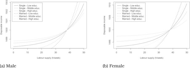
Preferences are defined over the positive ‘‘leisure time - disposable income’’ domain, with heterogeneity allowed in the leisure parameter. We estimate that utility increases with both disposable income and leisure time for almost all the individuals, as summarized in Table 5. Higher education in contrast decreases preferences for leisure time. We illustrate this with indifference curves of individuals with different education levels on Figure 3a and Figure 3b. Moreover, the number of children younger than 7 y.o. increases the importance of leisure time, except for single men.
Marginal utilities
| % Observations | Single Male | Single Female | Couples |
|---|---|---|---|
| <disp-formula> </disp-formula> | 100 | 100 | 100 |
| <disp-formula> </disp-formula> | 100 | 100 | Male: 99.89Female: 99.86 |
4.5.2. Opportunities
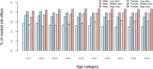
The estimated percentage of job offers in workers’ opportunity sets is given in Figure 4. One can observe that higher education strongly increases the number of job opportunities. For women, higher unemployment rates in an age category slightly decreases the number of job offers for those in that category, in line with the intuition that higher unemployment rates increase competition between unemployed and diminishes the probability to find suitable jobs. For men however, this effect is estimated to be smaller and opposite, resulting in young man having more job offers, despite higher unemployment rates.
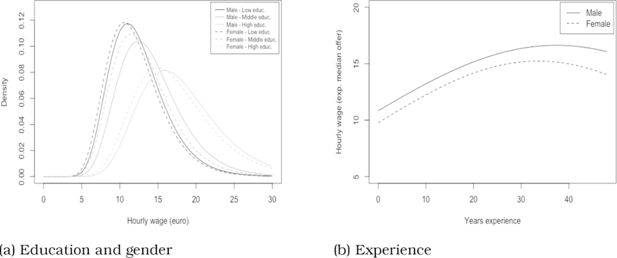
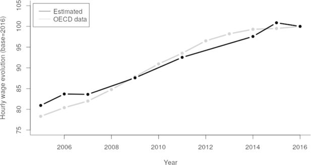
The estimated wage distributions and evolution are given in Figures 5 and 6. Education has the strongest positive impact on wage offers. Males also receive slightly higher wage offers than females. Years of (potential) experience, calculated as age minus expected age of labour market entry,21 have a positive impact on wage offers, up to a certain limit (34 for men and 35 for women) at which the person is close to retirement and possibly becomes less attractive for employers, resulting in lower wage offers.
The estimated hours distributions are illustrated on figure Figure 7a and Figure 7b . We estimate that men receive more full-time job offers than any other regime. The same holds for women, who however receive a significant amount of part-time offers.
4.5.3. Fit
A first check to see whether our model fits common perception of leisure and income preferences, is to verify the marginal utilities with respect to those variables are positive. Reasonably assuming most people would accept extra money or extra holidays ceteris paribus, those marginal utilities should be positive for a vast majority of people.22 The percentage of people for whom those marginal utilities are positive at the observed choices are in Table 5.
Secondly, Table 6 reports the estimated elasticities following an increase of of the wage offers. Besides total elasticities, we also report intensive margin elasticities, that reflect the average changes in labour supply of people who are already working. The third and fourth lines give the percentage (with respect to the total number of people in the gender-marital status category) of people starting/stopping to work. The estimated elasticities are in the range (and rather at the right of the distribution) of those estimated in the literature (see for example Keane, 2011).
Elasticities and participation changes (10 wage increase)
| Increase of male wages | Increase of female wages | |||||
|---|---|---|---|---|---|---|
| Single | Couple | Single | Couple | |||
| Male | Male | Female | Female | Male | Female | |
| Total elasticity | 0.270 | 0.117 | -0.072 | 0.210 | -0.067 | 0.163 |
| Intensive margin | 0.049 | 0.068 | -0.090 | 0.042 | -0.087 | 0.106 |
| Participation (entering, % of total) | 1.791 | 0.506 | 0.193 | 1.388 | 0.214 | 0.548 |
| Participation (leaving, % of total) | 0.025 | 0.000 | 0.531 | 0.000 | 0.535 | 0.000 |
Single men increase their labour supply slightly more than single women after an increase in wage offers, both at the intensive as at the extensive margin.23 Regarding married individuals, estimates indicate that married women would increase their labour supply more than men.24 This can be partly explained by the fact married women more often are out of the labour market or work part-time, and thus have more room to increase their supply of labour.
A number of married individuals will also react to an increase in their partners’ wage. This is due on one hand to an income effect, and on the other hand to the complementarity between partners’ leisure time. The income effect will tend to reduce the partners’ labour supply, while the effect of leisure complementarity will depend on the labour supply change of the first partner. Positive and negative labour supply reactions are predicted both at the intensive and extensive margin, but in both cases the negative effect dominates when looking at the aggregate level. Married individuals will thus on average decrease their labour supply or leave the labour market following an increase in their partners’ wage offers.
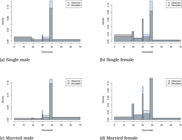
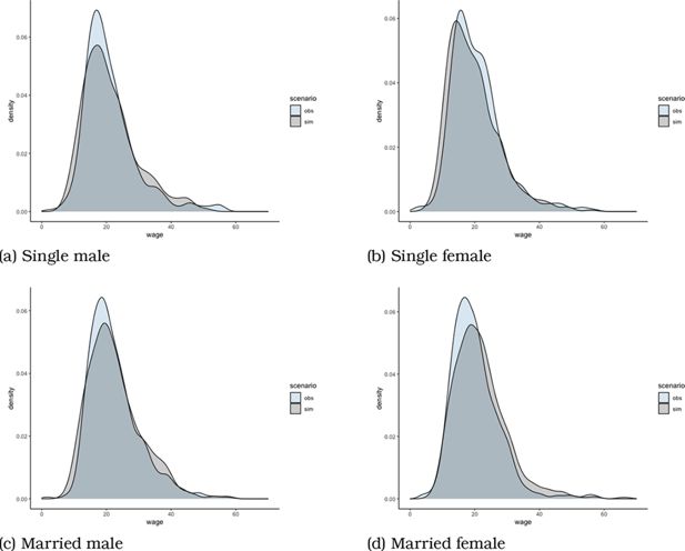
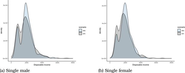
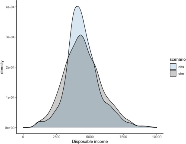
Lastly, we compare the observed distribution and the predicted distribution of some variables, using random draws for the stochastic part of the utility in the latter case. Density plots of observed and simulated hours worked, wages and disposable incomes are given in Appendix B.1 (Figures A3-A6).
5. Simulated policies
5.1. Reform scenarios
We simulate 3 hypothetical scenarios that increase the generosity of the work-bonus, named respectively reform , and .25 Those scenarios do not change the structure of the scheme, but only its generosity, in terms of base amount and/or in terms of eligibility thresholds, and are calibrated to have the same budgetary cost before behavioural changes, set at 300M EUR yearly. The first scenario consists of increasing the maximum amount of the reduction (parameter ), thereby further decreasing the participation tax rate for low earning capacity workers. The second scenario consists of increasing both the maximum amount and the thresholds proportionally (parameters , and ), which, besides further decreasing participation tax rates, also extends the scheme to higher earning capacity workers. Finally, in the third scenario the maximum amount is kept constant, but the eligibility range is increased (parameters and ).26
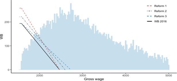
The base case policy is represented on Figure 8 together with the 3 reform scenarios. The continuous line represents the level of the existing WB granted to a full-time worker, in function of his gross monthly wage. The dotted lines represent the 3 hypothetical reform scenarios. The domain starts at the level of the minimum wage, and one can observe that the phase-out area starts soon after, as explained in Section 3. It can also be seen that reforms 1 and 3 will change the withdrawal rate of the policy, respectively to 29.2 and 16.9 , while reform 2 keeps this rate unchanged at 21.9 . Lastly, the bars represent the distribution of monthly FTE gross wages across the population, and show that our reforms will change the budget set of a significant number of individuals.
5.2. Theoretical predictions
Two effects can arise when changing the shape of the budget constraint of an individual working for a given hourly wage. If in the reform scenario, for a given amount of hours, income increases, a person working that amount of hours will feel richer and might reduce his labour supply in order to have more leisure time with an income higher or equal to the initial one. This effect is called the income effect, and is stronger when the marginal utility of income is relatively small, at the condition that leisure is a normal good. On the other hand, a reform of in-work benefits will also change the marginal return to work (corresponding to the slope of the budget constraint). An increase in the marginal return to work means that ‘‘not working’’ (or ‘‘leisure’’) implicitly costs more in terms of foregone wages. People facing a higher (lower) marginal return to work will therefore have a stronger incentive to work more (less). Those effects are called substitution effects. Note that besides those two effects, occurring on a budget constraint for a given wage, workers can also opt for jobs paying different wages.
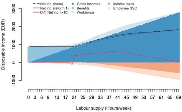
The change in budget constraint is illustrated for reform 1, for a single individual working at the minimum wage, on Figure 9. The dotted and continuous black lines represent the disposable incomes in the base and reform 1 scenarios, which is decomposed into different components in the reform case. We see that the reform renders many in-work options more attractive. The reason of the flat part on the left is that for small numbers of hours worked the benefit of the reform is offset by lower means-tested social assistance benefits. Then come part-time and full-time job situations where the reform has a strong and increasing (with labour supply) effect, which is straightforward given the design of the scheme. The benefit will start decreasing when working overtime. This result comes from the fact that the FTE wage, used for the determination of the WB level, is calculated by dividing gross earnings by contractual hours of work. People that have accepted a better paid job requiring frequent (informal) overtime, thus see their hourly wage over-estimated in that calculation.27 The option to work less and by doing so become eligible to the WB therefore becomes relatively more attractive. This third effect is not detectable with administrative data, where informal overtime is not taken into account. Lastly, note that for higher levels of hourly wages, the reform would have less impact, as the WB phases gradually out with hourly wages. Our reforms might thus incentivize individuals to switch to lower-paid jobs, that become relatively more attractive.
In summary, we can say that the options that become relatively more attractive following a WB increase are those that pay low wages, and that require hours that are not too low (as the means-tested benefits will offset the WB), nor too high (as the hourly wage will be overestimated in case of frequent overtime work).
5.3. Simulation procedure
We use a procedure proposed by Duncan and Weeks (1998) to simulate the behavioural changes resulting from our tax-benefit reforms. The procedure is essentially a Monte Carlo method relying on repeated random sampling of the random utility term. The different steps of this procedure are detailed next.
The first step of the procedure consists of, for each household, drawing a set of opportunities (market and out-of-market) from the estimated hours and wage distributions, conditionally on the observed opportunity being included. For each opportunity, we calculate the corresponding disposable income in the base and reform scenarios with the arithmetic micro-simulation model EUROMOD, of which the parameters are adapted in the case of the reform scenario. This allows to calculate the deterministic part of the utility function for each opportunity.
We then draw a vector of random utility terms from a Gumbel distribution in a way that guarantees that the total utility will be the highest for the observed choice, following a procedure proposed in Bourguignon et al. (2001). This operation is repeated times to get vectors of random Gumbel draws that predict choices that correspond to the observed choice.
Lastly, in each of the cases we predict which would be the ‘‘reform opportunity’’ chosen by the household by adding those random utility terms to the deterministic utilities under the reform scenario. This gives rise to a probability distribution over the set of opportunities of each household under the new tax-benefit system. This probability distribution then allows to calculate the expected hours of labour supply after the reform as well as expected income, tax and benefit amounts. Our simulations are run on the 2017 SILC dataset, which has income reference year 2016, and we set and .
5.4. Simulation results
5.4.1. Labour supply
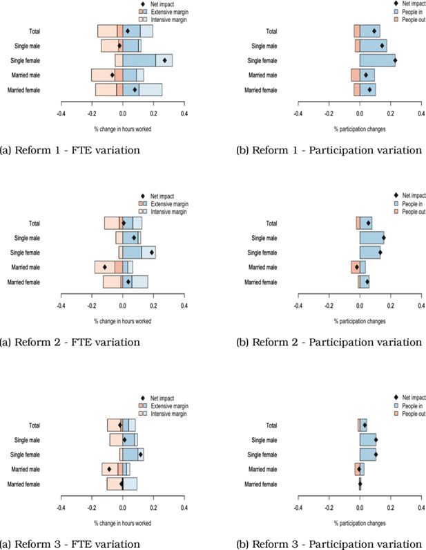
All 3 scenario’s predict an increase in labour supply if measured in terms of participation (number of people working positive hours). If measured in FTE, only scenario 1 and 2 predict an increase, while scenario 3 predicts a small decrease. An overview of the impact of the 3 different reforms is given in Table 7.28 Those effects are further decomposed for the different gender-marital status groups in Figure 10.
Effects of the reforms on labour supply
| Overview LS effects | Param. | Base | Ref1 | Ref2 | Ref3 |
|---|---|---|---|---|---|
| <disp-formula> </disp-formula> | 193.79 | 257.81 | 222.05 | 193.79 | |
| <disp-formula> </disp-formula> | 1577.89 | 1577.89 | 1577.89 | 1577.89 | |
| <disp-formula> </disp-formula> | 2461.27 | 2461.27 | 2590.07 | 2721.83 | |
| <disp-formula> </disp-formula> | 21.94 | 29.18 | 21.94 | 16.94 | |
| <disp-formula> </disp-formula> | 28.03 | 28.03 | 28.03 | 28.03 | |
| ΔLabour supply (FTE) | +669 (+0.032%) | +141 (+0.007%) | -362 (-0.017%) | ||
| - Ext. margin (FTE) | +1609 | +895 | +530 | ||
| - Int. margin (FTE) | -939 | -754 | -892 | ||
| ΔParticipation | +2024 (+0.093%) | +1200 (+0.055%) | +688 (+0.032%) | ||
| - people starting to work | 2831 | 1697 | 964 | ||
| - people stopping to work | 807 | 497 | 276 | ||
| ΔTotal gross labour income (M EUR) | -190.2 (-0.217%) | -166.3 (-0.190%) | -105.3 (-0.120%) | ||
| - average gross wage change (EUR/h) | -0.053 | -0.041 | -0.022 |
One can clearly observe that in all scenarios women increase their labour supply the most. The same holds for singles versus married. The first observation can be explained by the fact women receive lower wage offers on average and therefore potentially benefit from the increased workbonus more often. In addition, they start from higher unemployment/inactivity rates, and decreased participation tax rates have thus a higher potential effect on labour market entry. In addition, men have more jobs requiring overtime, and as explained in 5.2., such jobs can in certain cases become relatively less attractive than other jobs after a workbonus increase, leading overtime workers to switch to jobs requiring less hours.
The smaller or negative labour supply reactions of couples are mainly explained by stronger income effects: low-wage workers experience a revenue increase, resulting in a reduction of labour supply of one (or both) of the household members. Note also that married men reduce worked hours on average, which is explained by a partial substitution of male labour by female labour supply. Overall, the WB leads to a more homogeneous distribution of work.
Finally, one can observe total gross labour income decreases. This is driven by the decrease in average wages, due to a number of people switching to jobs that offer lower wages but desirable attributes, as those became relatively more attractive after the reform.
5.4.2. Welfare analysis
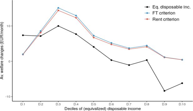
Besides equivalized disposable income,29 we present here, following Decoster and Haan (2014), two alternative welfare measures that account for leisure: the rent criterion and the full-time (FT) criterion.
The rent is the income that gives the same utility to an individual as a particular point in the ‘‘leisure-disposable income’’ space, when his labour supply is . In a standard representation of the labour supply decision with labour supply in abscissa and net income in ordinate, it is found at the intersection of the indifference curve passing through a given bundle and the vertical line at labour supply . The FT criterion is found at the intersection of the indifference curve with the vertical line at the level of full-time labour supply. The main reason to prefer those measures over traditional individual welfare metrics (for example equivalent or compensating variations, fixed preference orderings, …), is that they respect maximally the heterogeneous preferences of the agents, while bringing the normative choices, unavoidably present in all interpersonal comparisons, clearer to light.30 , 31 This can be intuitively understood by the fact those metrics use information on individual preferences, in the form of indifference curves, to translate the chosen ‘‘leisure-disposable income’’ combination into an ‘‘equivalent’’ income (rent or FT in this case). They moreover shed light on the normative assumptions made in the interpersonal comparison. For example, the rent-criterion gives maximal protection for people who give importance to leisure, and renders them minimally responsible for their aversion to work. The FT-criterion on the contrary treats industrious individuals (i.e. those having less distaste for work) more favourably.
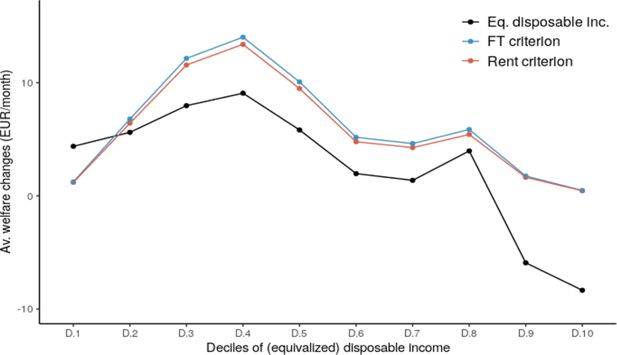
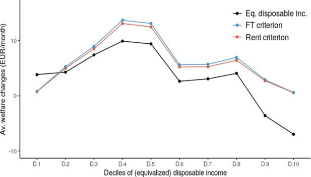
The welfare changes per equivalized disposable income decile are represented in Figure 11 for reform 1. The same graphs are provided for reforms 2 and 3 in Appendix B (Figure A1 and A2) . One can see that the reform has the strongest impact on lower middle class individuals. The poorest individuals, of whom a significant share is out of the labour market because of stronger preferences for leisure and/or fewer job opportunities,32 do not see their welfare increase much. The reason is that the welfare gains resulting from disposable income increases following the acceptance of a job are almost offset by the welfare losses due to the decrease in leisure time. The third and fourth decile individuals on the contrary have higher employment rates, and many will thus benefit from a higher disposable income, without sacrificing leisure time. In the highest deciles, the average disposable income decrease is explained by a number of individuals opting for lower-paid jobs that have more attractive attributes. Welfare gains are thus small when measured with the FT and Rent criteria: gains in welfare due to preferred job-attributes barely exceed the losses due to the disposable income decreases.
In Table 8, we compute the population-wide weighted Gini-coefficient and poverty rate (assuming people out of the model do not change their labour supply). The Gini is calculated on equivalized incomes (using the OECD-modified scale), and the poverty rate is defined as the percentage of people having an equivalized income lower than 60% of the median equivalized income. All the reforms reduce inequalities and poverty by a small amount, with reform 1 reducing inequalities and poverty the most. This limited impact is due to the fact the purchasing power gains resulting from the WB scheme are, even though concentrated at the left of the wage distribution, quite spread over the equivalized income distribution.
Effects of the reforms on poverty and inequality
| Poverty and Inequality | Base | Ref1 | Ref2 | Ref3 |
|---|---|---|---|---|
| Gini | 21.25 | 21.18 | 21.19 | 21.20 |
| Poverty rate | 10.37 | 10.20 | 10.22 | 10.26 |
5.4.3. Budget
The total budget necessary for each reform was set at 300M EUR yearly before behavioural changes.33 The decomposed effects on the government budget, both before and after behavioural changes (where we assume individuals not included in the labour supply model do not change labour supply), are given in Table 9. None of the reforms pays for itself. In other words, the reduction of government expenses that follow such reforms, resulting from a decrease in social assistance and unemployment benefits, do not compensate the decreases in revenues from taxes and social security contributions. Those decreases are due to a direct effect resulting from the WB extension that reduces taxes and social security contributions paid by employees. In addition, workers will choose lower-paid jobs on average, which will reduce social security contributions, and to a lesser extent taxes, paid by employees even more. Those effects are not compensated by the additional taxes and social security contributions paid by new entrants.
Effects of the reforms on budget balance (Million EUR)
| Budget Balance | Ref1 | Ref2 | Ref3 |
|---|---|---|---|
| +Δ Social Security contrib. (static) | -83.4 | -82.4 | -82.9 |
| +Δ Personal Income Tax (static) | -234.9 | -233.2 | -232.1 |
| –Δ Benefits (static) | -16.7 | -15.9 | -15.2 |
| =Δ Budget balance (static)* | -301.5 | -299.7 | -299.7 |
| Additional impact following LS changes | |||
| +Δ Social Security contrib. | -176.1 | -168.8 | -160.4 |
| +Δ Personal Income Tax | +40.9 | +53.0 | +82.3 |
| –Δ Benefits | -23.8 | -17.8 | -12.7 |
| =Δ Budget balance (total)* | -413.0 | -397.7 | -365.2 |
-
*
A negative balance corresponds to a deficit for the government.
5.5. Discussion
All 3 reforms predict labour supply increases when measured in participation. Reform 3 however, predicts a labour supply decrease when measured in FTE. An interesting complementary statistic for the parsimonious policy makers that see in-work benefits mainly as a labour market activation policy is the average net cost to increase labour supply by a FTE or alternatively, by a participant. Note however, that the denominator of this indicator can be close to in reforms that create positive and negative labour supply changes that on average almost compensate each other, as in our reform 3, and to a lesser extent, reform 2, resulting in high numbers.
We obtain costs per additional FTE ranging from 368.5 thousand EUR in reform 1 to 1660.1 thousand EUR in reform 2 . In reform 3 the ratio is not calculated as number of FTE decreases. Other studies on relatively similar schemes find lower numbers for Belgium. For example Orsini (2006b) and Dagsvik et al. (2011), estimate costs per FTE to be located respectively between 136.0 and 204.1 and between 35.5 and 171.3 thousand EUR depending on the in-work benefit structure and structural model used.34 Regarding neighbour countries, Orsini (2006b) estimates costs per FTE in the the order of 272.1 thousand EUR for the WFTC, 231.3 thousand EUR for the German Mini-Jobs tax reform and 163.2 thousand EUR for the French PPE.
Costs per new participant are estimated in our simulation to lie between 121.1 and 560.7 thousand EUR, corresponding respectively to reforms 1 and 3 (Table 10). Only Dagsvik et al. (2011) gives numbers for Belgium, located between 18.8 and 36.3 thousand EUR. For Other European countries, Bargain and Orsini (2006) estimate it to vary from 88.9 for France and 127.1 for Germany to 234.4 thousand EUR for Finland. Compared to previous studies and simulations of in-work benefits, we thus estimate rather high costs per FTE and per new participant.
Net costs to increase labour supply (Thousand EUR)
| Net costs | Ref1 | Ref2 | Ref3 |
|---|---|---|---|
| Cost / additional FTE | 368.5 | 1660.1 | - |
| Cost / additional participant | 121.1 | 195.1 | 560.7 |
An important difference with some previous research (for example, Orsini (2006a); Orsini (2006b) and Bargain and Orsini (2006)) is that our simulation allows people to not only change worked hours, but also opt for lower paid jobs (with preferable attributes). In section 5.4 we showed that this would make the reform more costly, as people opt for lower-paid jobs, which mechanically decreases tax and social security contribution revenues of the government. This consequently increases the overall cost/additional worker of the reform. Particular attention should therefore be paid to this effect, especially when analyzing reforms that significantly change the relative attractiveness of jobs offering low wages, as is the case of the Belgian WB.
Those differences might also be explained by a modelling decision regarding how overtime workers are taken into account. It is common when using survey data to exclude people declaring ‘‘unrealistic’’ amounts of hours and it is necessary to round the observed values to values in the choice set when using a discrete hours choice model (in Orsini (2006a) and Orsini (2006b) people working >80h/week are excluded from the sample and the hours of those working between 45 and 80 hours are rounded to 50 hours), while in administrative data informal overtime workers are not detected, (as in Dagsvik et al. (2011)). Those limits result in potentially underestimated intensive margin elasticity estimations, as one do only take into account overtime workers reducing their labour supply to a limited extent.
As suggested by Decoster and Vanheukelom (2019) about the proposed Flemish WB extension, higher costs per additional FTE or participant might also be explained by decreasing marginal utility of income, meaning that further increasing in-work benefits will probably not have effects of the same magnitude as the initial introduction of those benefits. Along the same line, it could be explained by the purchasing power increases (following real wage increases) over the last decades that decreased marginal utility of income at a given labour supply level.
Finally, those estimate differences are probably partly explained by differing initial situations and reforms simulated: an in-work benefit is more likely to have a positive impact on employment in situations where more people are jobless. On the contrary, in an economy with full employment, the benefit will be costly and mainly create negative income effects.
6. Conclusion
In this paper, we discussed the history and the particularity of in-work benefit schemes in Belgium and simulated the effects of 3 different extensions of the work-bonus scheme, varying in terms of eligibility ranges and benefit amounts. We showed that such reforms would slightly increase labour supply when measured in terms of participation. When measured in terms of full-time equivalent workers, labour supply decreases in one of the 3 scenario’s and slightly increases in the 2 others. Those small net effects are the result of opposing effects, both at the intensive and extensive margin.
We then calculated that the cost of such reforms is significant, and that savings in social assistance and unemployment benefits resulting from higher employment rates are far from compensating the important decreases in social security contributions and personal income taxes. Those decreases are exacerbated by the fact some workers will opt for lower-paid jobs, that become relatively more attractive with the work-bonus extension. This results in costs per FTE and new participant that are considerable, starting at 368.5 thousand EUR per FTE and 121.1 thousand EUR per new participant. Compared to previous studies, those figures are rather high. We gave different arguments why those figures could however be more accurate than previous estimations in subsection 5.5. We moreover calculated that the welfare gains are the highest for the third and fourth welfare deciles, while the first decile is almost unaffected.
The natural question that arises is whether increasing the workbonus is the most effective way to reach poverty reduction and labour market participation goals. One can reasonably wonder if investing in other active labour market policies as training programmes, additional coaching, more targeted wage subsidies or public jobs, possibly combined with investments in poverty-alleviating programmes, could not be a more adequate government spending.
Footnotes
1.
Note that flexibilization can concern wage regulations, hours regulations, conditions of dismissal,... and that less regulation is not necessarily synonym of more jobs: there is for example, no unanimity about the effect of minimum wages on employment (Neumark and Wascher, 2006)
2.
Other measures in this category consist for example of lowering unemployment benefits or rendering them decreasing over time.
9.
Note that this measure is not the same as the “Federale Jobkorting”, the name given to an increase in the amount of deductible professional expenses.
10.
The measure was accused to discriminate people working in Flanders but living outside Flanders, as those would not have the right to the jobkorting.
11.
Other measures part of this tax shift include: decreases of the personal income taxes through expansions of the brackets and the abolition of the 30-% bracket, decreases of the social security contributions for employers and self-employed, the introduction of an increased and uniform tax free amount, etc.
12.
See also the reworked version Vandelannoote and Verbist (2019).
13.
The amount of the basic reduction is slightly different for blue and white collar workers. Since it is not possible to distinguish between these types based on SILC data, only the amount forwhite collar workers is given here and simulated in EUROMOD.
14.
We use the data as different cross-sections (we abstract from the fact that a share of individuals might appear in different surveys).
15.
Estimated based on figures 2 and 3 in Dagsvik et al. (2011). Note also that there are very specific situations where for technical and organizational reasons the law authorizes derogations to the 38 (to 40) hours week, but those should mostly be compensated by periods of rest in a way that average weekly hours do not exceed the legal working week.
16.
As the social desirability bias (a tendency of survey respondents to answer questions in a manner that will be viewed favorably by others) that could for example result from individuals desiring to be seen as hard-working.
17.
We abandon i, j and k subscripts for clarity.
18.
EU-wide arithmetic tax-benefit model widely used by the European commission for policy analysis and developed and managed by the Institute for Social and Economic Research (ISER) at the University of Essex.
19.
Arrêté royal du 23 Juillet 2012 modifiant l’arrêté royal du 25 novembre 1991 portant la réglementation du chômage dans le cadre de la dégressivité renforcée des allocations de chômage, Moniteur belge, 30 Juillet 2012. (Royal decree of 23 July 2012 modifying Royal decree of 25 November 1991 relating to unemployment benefits in the context of the reinforcement of degressivity of unemployment benefits)
20.
We use uniform distributions for the hours (from 0 to 70) and hourly wages (from 0 to 60). The prior probability to draw an out-of-market offer is set at 0.10.
21.
Estimated at 15 for low educated individuals (ISCED levels 0,1,2), 19 of middle educated individuals (ISCED levels 3,4,5), and 23 for high educated individuals (ISCED level 6).
22.
The exception in our eyes that could be significant is the case of unemployed finding no suitable job offer. In that case the unemployed might be desiring to find a good job, which provides a feeling of accomplishment, even if it would not be associated with an income increase. Also, young workers could be desiring to work many hours, even without additional salary, to build human capital and increase future utility.
23.
Note that the number of men that stop working after a wage increase is slightly positive. This seemingly counter-intuitive result is due to the fact disposable income does not always increase monotonically with labour income due to discontinuities in certain means-tested benefits (for example due to a yearly 250EUR exemption in the means-test for social assistance).
24.
We use the adjective married to refer to members of the couples. Those can also be in a consensual union.
25.
Note that we use 2016 as reference scenario, even though the workbonus has (very) slightly and gradually been augmented during the 2015-2019 tax-shift.
26.
Note that in the reference scenario, the WB cannot exceed social security contributions due, and the FWB cannot exceed 640 EUR/year. In our reforms we allow the WB and FWB to be refundable benefits in case they would outreach those limits.
27.
As an illustration, imagine a low-level manager earning a gross wage of 2500 EUR per month for a job that requires on average 200 hours of work monthly (of which some informal overtime). This person’s hourly wage equals 12,5 EUR/hour. However, as the legal or contractual working week counts 38 hours (about 165 per month), his earning capacity in the eyes of the fiscal authority will be estimated at more than 15 EUR/hour, excluding him from the WB scheme.
28.
Not all workers are included in our simulation sample (see section 4.1.). Our filtering procedure keeps 64.9% of individuals who are labour market available, for that dataset. If one would be interested in having the absolute changes in labour supply for the whole population, a possibility would be to divide the predictions of the model in Table 7 by 64.9%, which would be relatively accurate if people excluded from the sample have comparable reactions to the reforms on average.
29.
We use the term equivalized income to denote the income divided by an equivalence scale, in order to take into account economies of scale in household expenses.
30.
Normative analysis in a framework of heterogeneous preferences poses the difficult problems of comparability and aggregation of individual utilities (due to an incompatibility between two sets of axioms, one related to the respect of individual preferences and one related to interpersonal comparability, see Fleurbaey and Trannoy (2003)), that are often neglected (e.g. when simply aggregating compensating variations). One way to address these problems is to use a reference preference ordering (or a reference agent/household). The disadvantage of this choice is, however, that it would create an inconsistency between the positive part of our analysis, where household heterogeneity plays a role in the decision process, and the normative part of our analysis, where this heterogeneity is set aside. Fleurbaey (2006), and Fleurbaey (2007) propose another way to escape this incompatibility problem, by restricting (but retaining maximally) preference heterogeneity to what they call Subset Dominance. It is argued that giving priority to respecting preferences is less arbitrary and allows to shed light on the ethical priors used (and thus the cut between personal and social responsibility) when selecting the subsets: The rent-criterion for example gives maximal protection for people who give importance to leisure, and renders them minimally responsible for their aversion to work. The FT-criterion on the contrary treats industrious individuals (i.e. those having less distaste for work) more favourably.
31.
For a detailed overview of the normative foundations of the three most popular approaches to measure well-being in a multidimensional setting: the capability approach, the subjective well-being approach and the equivalent income approach, see Decancq et al. (2015). For a discussion on welfare analysis applied to Random Utility Models of Labour Supply, see Decoster and Haan (2010).
32.
In the lowest decile, individuals have an education level below average. Our estimates suggests that this results in stronger preferences for leisure and less job opportunities. Moreover, in the lowest decile, couples have more children than the average, which also contributes to higher preferences for leisure.
33.
This is done by running EUROMOD iteratively and adapting tax-benefit parameters at each loop in order to approach a pre-defined budget deficit (300M EUR). We used a tolerance level of 1% (3M EUR).
34.
Numbers from their publications are transformed in 2016 EUR with CPI indices to be comparable with ours. Orsini (2006a) database is from 2000, Dagsvik et al. (2011) from 2001 and Bargain and Orsini (2006) from 1998.
3.
An unemployment trap is a situation in which a generous social security scheme (relatively to wages) lowers the financial difference between working and being inactive.
4.
Or equivalently, using “full-time equivalent” (FTE) labour income, the gross salary an employee would receive if he worked full-time at his gross hourly wage.
5.
However this wide consensus among economists has recently been affected by new study of Henrik Kleven showing that employment increases align closely with the confounding effects of welfare reforms and a booming macro-economy. He concludes that the case for sizable extensive margin effects of the EITC is fragile (Kleven, 2019).
6.
The scheme changed a couple of times, and its name changed successively to Family Credit and Working Families Tax Credit, before its final name Working Tax Credit (combined with Child Tax Credit). Most of the evaluations of employment effects refer to the period where the IWB was named WFTC, and was significantly increased.
7.
Loi du 20 Décembre 1999 visant à octroyer [un bonus à l’emploi sous la forme d’] une réduction des cotisations personnelles de sécurité sociale aux travailleurs salariés ayant un bas salaire [et à certains travailleurs qui ont été victimes d’une restructuration].
8.
Loi du 10 Août 2001 portant réforme de l’impôt des personnes physiques.
Appendix A
Parameter estimates
Below tables give an overview of parameter estimates. The Log-Likelihood at the maximum found is -29450.05. Note that for education covariates, "Middle education" is the reference, and for region covariatas, "Flanders" is the reference, meaning that the effects of those covariates are measured comparatively to middle-educated Flemish people.
Table A1 Parameter estimates - Preferences singles
| Preferences | Estimate | Standard Error | t-value |
|---|---|---|---|
| Single male | |||
| Leisure | |||
| Constant | 8.380 | 2.074 | 4.041 |
| Log(age) | -4.654 | 1.145 | -4.065 |
| Log(age)2 | 0.665 | 0.158 | 4.208 |
| Children 4-6 | -0.117 | 0.073 | -1.611 |
| Children 7-9 | 0.002 | 0.072 | 0.034 |
| Wallonia | 0.125 | 0.035 | 3.578 |
| Brussels | 0.058 | 0.030 | 1.901 |
| Low education | 0.072 | 0.040 | 1.799 |
| High education | -0.044 | 0.026 | -1.670 |
| Exponent | -9.217 | 0.414 | -22.262 |
| Income | |||
| Constant | 1.526 | 0.057 | 26.696 |
| Exponent | 0.721 | 0.036 | 20.250 |
| Single female | |||
| Leisure | |||
| Constant | 24.608 | 4.348 | 5.660 |
| Log(age) | -13.548 | 2.392 | -5.665 |
| Log(age)2 | 1.913 | 0.331 | 5.784 |
| Children 0-3 | 0.297 | 0.104 | 2.864 |
| Children 4-6 | 0.155 | 0.078 | 1.982 |
| Children 7-9 | 0.116 | 0.064 | 1.824 |
| Wallonia | 0.145 | 0.047 | 3.093 |
| Brussels | -0.025 | 0.040 | -0.613 |
| Low education | 0.321 | 0.088 | 3.646 |
| High education | -0.332 | 0.052 | -6.400 |
| Exponent | -9.005 | 0.351 | -25.662 |
| Income | |||
| Constant | 1.604 | 0.062 | 25.748 |
| Exponent | 0.681 | 0.037 | 18.356 |
Table A2 Parameter estimates - Preferences couples
| Preferences | Estimate | Standard Error | t-value |
|---|---|---|---|
| Couples | |||
| Leisure | |||
| Constant leisureM | 5.637 | 0.110 | 51.210 |
| Log(age) | -3.117 | 0.061 | -51.380 |
| Log(age)2 | 0.443 | 0.011 | 41.785 |
| Children 0-3 | 0.012 | 0.009 | 1.287 |
| Children 4-6 | 0.003 | 0.010 | 0.326 |
| Children 7-9 | 0.003 | 0.009 | 0.343 |
| Wallonia | 0.042 | 0.011 | 3.738 |
| Brussels | 0.036 | 0.015 | 2.347 |
| Low education | 0.053 | 0.018 | 2.885 |
| High education | -0.003 | 0.010 | -0.293 |
| Constant leisureF | 13.996 | 5.220 | 2.681 |
| Log(age) | -7.480 | 2.900 | -2.579 |
| Log(age)2 | 1.100 | 0.403 | 2.730 |
| Children 0-3 | 0.137 | 0.049 | 2.821 |
| Children 4-6 | 0.151 | 0.052 | 2.882 |
| Children 7-9 | 0.031 | 0.046 | 0.676 |
| Wallonia | 0.123 | 0.053 | 2.303 |
| Brussels | -0.159 | 0.064 | -2.508 |
| Low education | 0.091 | 0.103 | 0.888 |
| High education | -0.402 | 0.064 | -6.275 |
| Exponent leisureM | -10.872 | 0.243 | -44.764 |
| Exponent leisureF | -8.371 | 0.264 | -31.751 |
| Income | |||
| Constant | 3.016 | 0.122 | 24.687 |
| Exponent | 0.561 | 0.028 | 20.351 |
| Cross-effect | |||
| Cross-effect leisure | 0.032 | 0.005 | 6.541 |
Table A3 Parameter estimates - Opportunities
| Opportunities | Estimate | Standard Error | t-value |
|---|---|---|---|
| Male | |||
| Intensity | |||
| Working | -3.899 | 0.090 | -43.151 |
| Group specific unemp. | 0.011 | 0.004 | 2.898 |
| Wallonia | -0.626 | 0.088 | -7.133 |
| Brussels | -1.084 | 0.102 | -10.655 |
| Low education | -0.894 | 0.094 | -9.477 |
| High education | 0.484 | 0.102 | 4.758 |
| Offered time regimes | |||
| Part-time dummy 1 | 0.618 | 0.092 | 6.725 |
| Part-time dummy 2 | 0.909 | 0.082 | 11.106 |
| Full-time dummy | 2.543 | 0.031 | 80.733 |
| Offered wages | |||
| Constant | 2.407 | 0.017 | 143.643 |
| Low education | -0.121 | 0.011 | -11.476 |
| High education | 0.247 | 0.007 | 33.057 |
| Experience | 2.290 | 0.140 | 16.404 |
| Experience2 | -3.063 | 0.307 | -9.969 |
| Standard dev. | 0.295 | 0.001 | 315.096 |
| Female | |||
| Intensity | |||
| Working | -3.237 | 0.077 | -42.108 |
| Group specific unemp. | -0.021 | 0.003 | -6.481 |
| Wallonia | -0.540 | 0.077 | -7.050 |
| Brussels | -0.879 | 0.094 | -9.383 |
| Low education | -0.677 | 0.090 | -7.522 |
| High education | 0.565 | 0.089 | 6.352 |
| Offered time regimes | |||
| Part-time dummy 1 | 1.496 | 0.050 | 30.180 |
| Part-time dummy 2 | 1.731 | 0.055 | 31.664 |
| Full-time dummy | 2.055 | 0.033 | 61.666 |
| Offered wages | |||
| Constant | 2.303 | 0.016 | 141.385 |
| Low education | -0.079 | 0.012 | -6.793 |
| High education | 0.273 | 0.008 | 33.886 |
| Experience | 2.650 | 0.131 | 20.200 |
| Experience^2 | -3.950 | 0.295 | -13.400 |
| Standard dev. | 0.304 | 0.001 | 395.650 |
Table A4 Parameter estimates - Wage eq. year dummies (Ref year: 2017)
| Opportunities | Estimate | Standard Error | t-value |
|---|---|---|---|
| Wage eq. year dummies | |||
| 2006 dummy | -0.212 | 0.010 | -21.924 |
| 2007 dummy | -0.178 | 0.009 | -19.012 |
| 2008 dummy | -0.179 | 0.009 | -19.061 |
| 2010 dummy | -0.133 | 0.009 | -14.050 |
| 2012 dummy | -0.078 | 0.010 | -7.982 |
| 2015 dummy | -0.025 | 0.010 | -2.580 |
| 2016 dummy | 0.009 | 0.010 | 0.908 |
Appendix B
Welfare changes
Simulated distributions
To test the fit of the model, we take a vector of random Gumbel draws and add them to the deterministic utilities of the different options in decision maker’s choice sets. We then compare the simulated distribution and observed distribution of some key variables. Note that we estimate the model using 7 cross-section data sets of years ranging from 2005 to 2015, while we here simulate distributions for 2015.
References
-
1
Labour supply in Italy: an empirical analysis of joint household decisions, with taxes and quantity constraintsJournal of Applied Econometrics 14:403–422.https://doi.org/10.1002/(SICI)1099-1255(199907/08)14:4<403::AID-JAE520>3.0.CO;2-4
-
2
Les effets incitatifs de la prime pour l’emploi: une évaluation difficileEconomie et Statistique 412:57–80.https://doi.org/10.3406/estat.2008.7042
-
3
In-work policies in Europe: killing two birds with one stone?Labour Economics 13:667–697.https://doi.org/10.1016/j.labeco.2005.10.007
-
4
Fast development with a stable income distribution: Taiwan, 1979-94Review of Income and Wealth 47:139–163.https://doi.org/10.1111/1475-4991.00009
-
5
Did working families’ tax credit work? The impact of in-work support on labour supply in Great BritainLabour Economics 13:699–720.https://doi.org/10.1016/j.labeco.2005.11.002
-
6
The convergence of a class of double-rank minimization algorithmsIMA Journal of Applied Mathematics 6 :222–231.https://doi.org/10.1093/imamat/6.3.222
-
7
Estimating and simulating with a random utility random opportunity model of job choice presentation and application to BelgiumInternational Journal of Microsimulation 9:144–191.https://doi.org/10.34196/ijm.00139
-
8
The Earned Income Tax Credit (EITC): an economic analysis. Congressional Research Service
-
9
Subsidies on low-skilled workers’ social security contributions: the case of BelgiumEmpirical Economics 40:779–806.https://doi.org/10.1007/s00181-010-0367-6
-
10
Labor supply with non-convex budget sets, hours restriction and non-pecuniary job-attributesDiscussion Papers 76:1.
-
11
Handbook of income distribution67–140, Inequality, income, and well-being, Handbook of income distribution, 2, p, https://doi.org/10.1016/B978-0-444-59428-0.00003-5.
-
12
Empirical welfare analysis in random utility models of labour supplySSRN Electronic Journal 17:1.https://doi.org/10.2139/ssrn.1736554
-
13
Welfare effects of a shift of joint to individual taxation in the German personal income taxFinanzArchiv 70:599–624.https://doi.org/10.1628/001522114X685500
-
14
De jobbonus: nuttig medicijn of overdosis?De jobbonus: nuttig medicijn of overdosis?, http://www.andredecoster.be/publication/de-jobbonus-nuttig-medicijn-of-overdosis/.
-
15
In-work tax credits in Belgium: an analysis of the Jobkorting using a discrete labor supply modelBrussels Economic Review 55:121–151.
-
16
Simulating transitions using discrete choice modelsJournal of the American Statisitcal Association 1.
-
17
A new approach to variable metric algorithmsThe Computer Journal 13:317–322.https://doi.org/10.1093/comjnl/13.3.317
-
18
Social welfare, priority to the worst-off and the dimensions of individual well-beingInequality and Economic Integration, London: Routledge.
-
19
Social choice and the indexing dilemmaSocial Choice and Welfare 29:633–648.https://doi.org/10.1007/s00355-007-0248-x
-
20
The impossibility of a Paretian egalitarianSocial Choice and Welfare 21:243–263.https://doi.org/10.1007/s00355-003-0258-2
-
21
La dégressivité renforcée des allocations de chômage: impact sur La pauvretéRevue Belge de Securite Sociale 2:273.
-
22
A family of variable-metric methods derived by variational meansMathematics of Computation 24 :23–26.https://doi.org/10.1090/S0025-5718-1970-0258249-6
-
23
A good time for making work pay? Taking stock of in-work benefits and related measures across the OECDOECD Social, Employment and Migration Working Papers 81:1.https://doi.org/10.1787/225442803245
-
24
Labor supply and taxes: a surveyJournal of Economic Literature 49:961–1075.https://doi.org/10.1257/jel.49.4.961
-
25
The EITC and the extensive margin: a reappraisalNational Bureau of Economic Research Working Paper 1.https://doi.org/10.3386/w26405
-
26
Gender and flexibility in working time in BelgiumTechnical report ULB–Universite Libre de Bruxelles 1.
-
27
Minimum wages and employment: a review of evidence from the new minimum wage researchNational Bureau of Economic Research Working Paper Series 1.https://doi.org/10.3386/w12663
- 28
-
29
Tax-Benefits reforms and the labor market: evidence from Belgium and other EU countriesSSRN Electronic Journal 3988:1.https://doi.org/10.2139/ssrn.898847
-
30
Conditioning of quasi-newton methods for function minimizationMathematics of Computation 24:647.https://doi.org/10.2307/2004840
-
31
Evaluating the impact of the French Tax credit on the employment rate of womenJournal of Public Economics 92:2036–2047.https://doi.org/10.1016/j.jpubeco.2008.02.007
-
32
Low-skilled jobs: the French strategyObservatoire Français des Conjonctures Economiques 1.
-
33
The design of in-work benefits: how to boost employment and combat poverty in BelgiumImPRovE Working Paper 1.
-
34
Werkt het design van de werkbonus om tewerkstelling te stimuleren en armoede te bestrijden in België?Belgisch tijdschrift voor Sociale zekerheid 1.
Article and author information
Author details
Funding
This work was supported by UCLouvain Saint-Louis Bruxelles, FSR grant (fonds spécial de recherche).
Acknowledgements
I am grateful to André Decoster, Tom Truyts, Bruno Van der Linden, Gilles Grandjean, Koen Declercq, Toon Vanheukelom, Sebastiaan Maes, Bart Capéau, Liebrecht De Sadeleer and David Sonnewald for their introduction into and/or discussions about micro-simulation, RURO-modelling and labour economics literature, as well as their regular feedback and comments. The usual disclaimer applies.
The results presented here are based on EUROMOD version I2.0+. EUROMOD is maintained, developed and managed by the Institute for Social and Economic Research (ISER) at the University of Essex, in collaboration with national teams from the EU member states. We are indebted to the many people who have contributed to the development of EUROMOD. The process of extending and updating EUROMOD is financially supported by the European Union Programme for Employment and Social Innovation "EaSI" (2014-2020). The results and their interpretation are the author’s responsibility.
Publication history
- Version of Record published: April 30, 2021 (version 1)
Copyright
© 2021, de Mahieu
This article is distributed under the terms of the Creative Commons Attribution License, which permits unrestricted use and redistribution provided that the original author and source are credited.


