The Complexity of Incorporating Carbon Social Returns in Farm Afforestation: A Microsimulation Approach
- Teagasc, Ireland
- National University of Ireland, Ireland
Figures

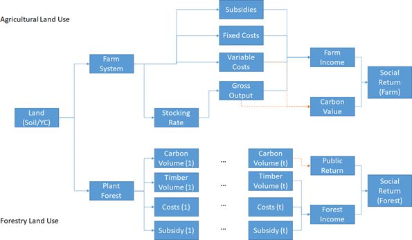
Structure of the Forestry Land use Change Microsimulation Model

Total carbon (C) storage curves for unthinned (u) and thinned (t) Sitka spruce yield class 8, 16 and 24

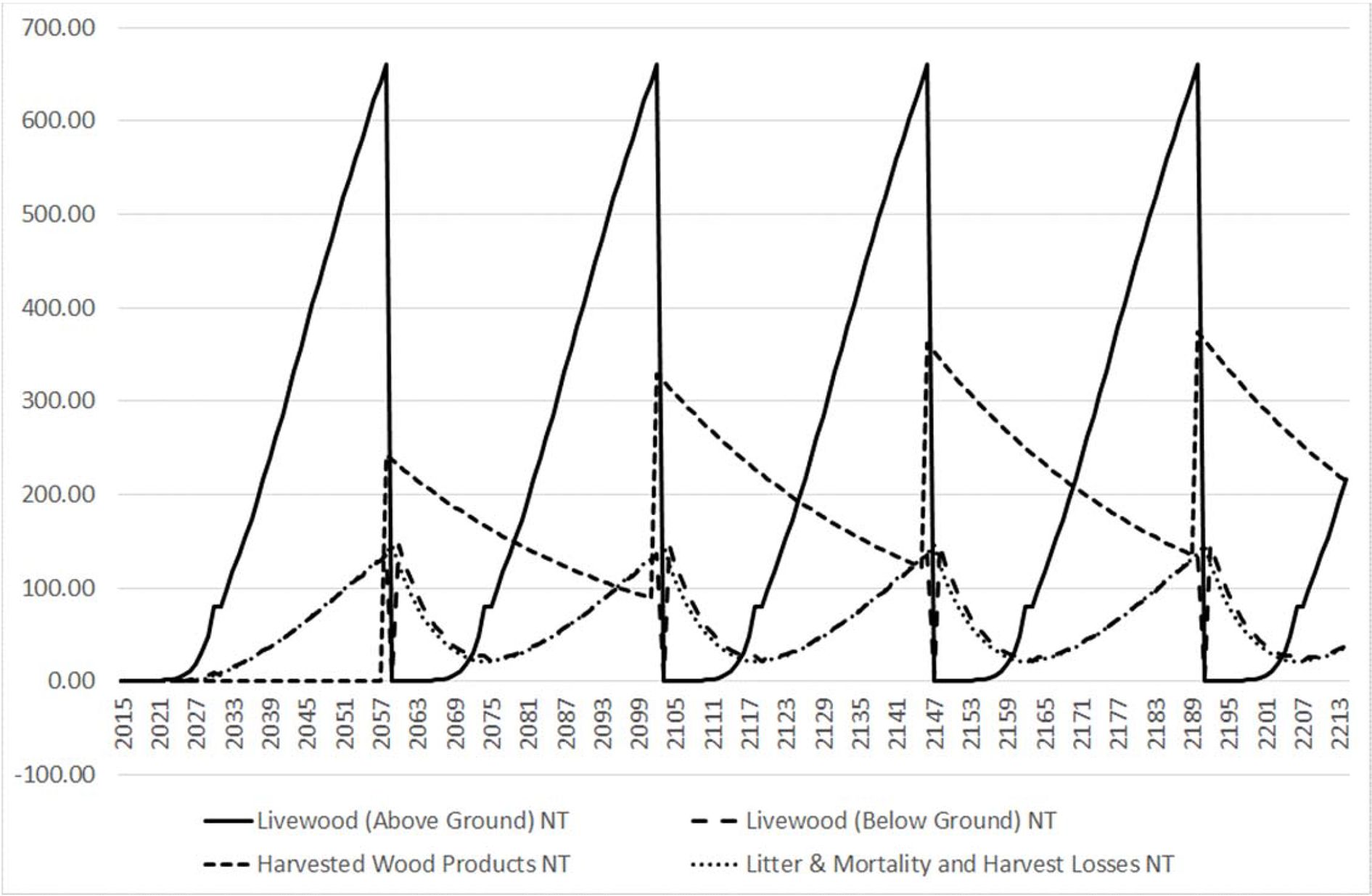
Carbon (C) Sequestration/Loss for No Thin (NT) Yield Class 18 over 200 years
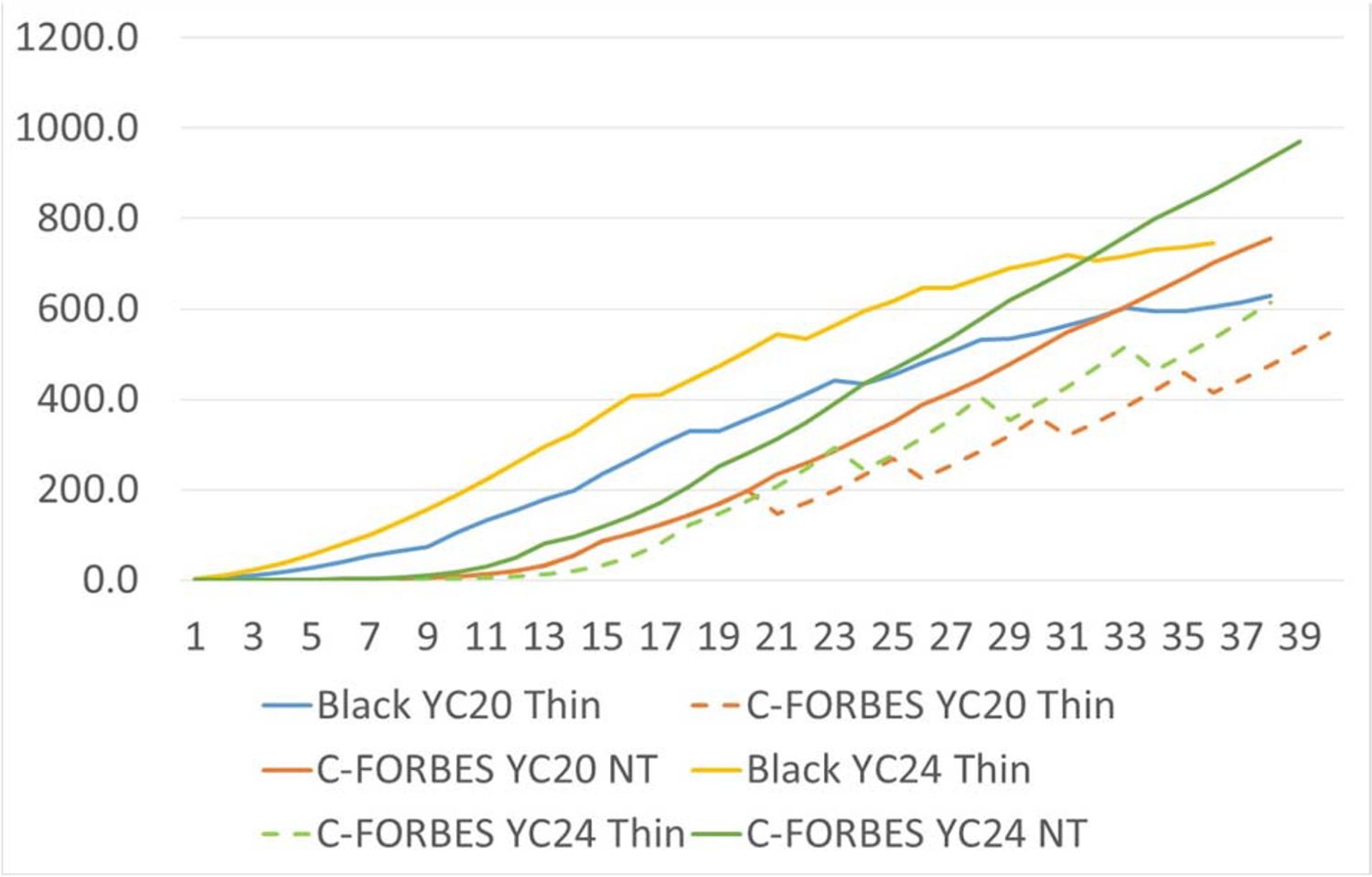
Comparison of Above Ground tCO 2 (C-ForBES and Teagasc Forest Carbon Tool) over one rotation

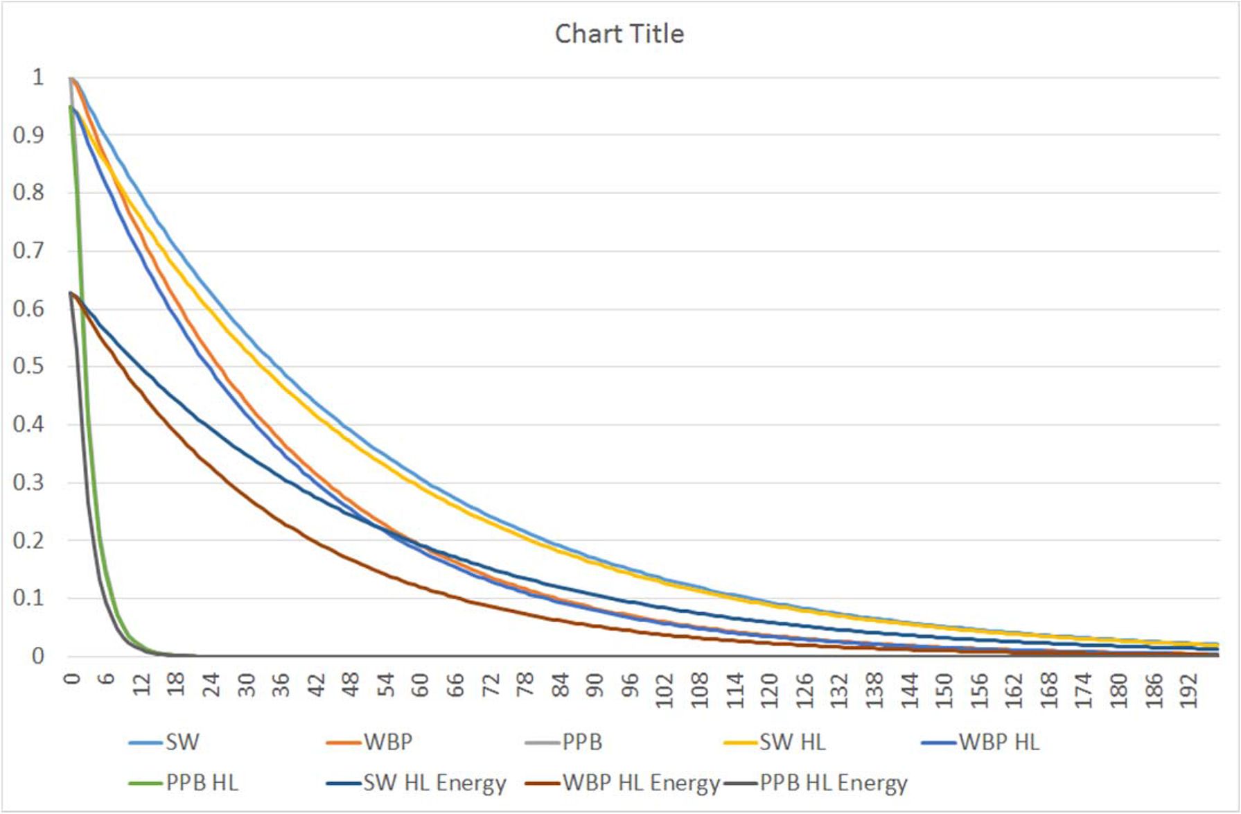
Impact of different approaches to determine the wood inputs to HWP on SW, WBP, PPB Carbon Liberation Curves for NIR (2018) WBP, PPB Carbon Liberation Curves for NIR (2018) approach, C-ForBES harvest losses (HL) and C-ForBES harvest losses + wood energy losses (HL Energy)

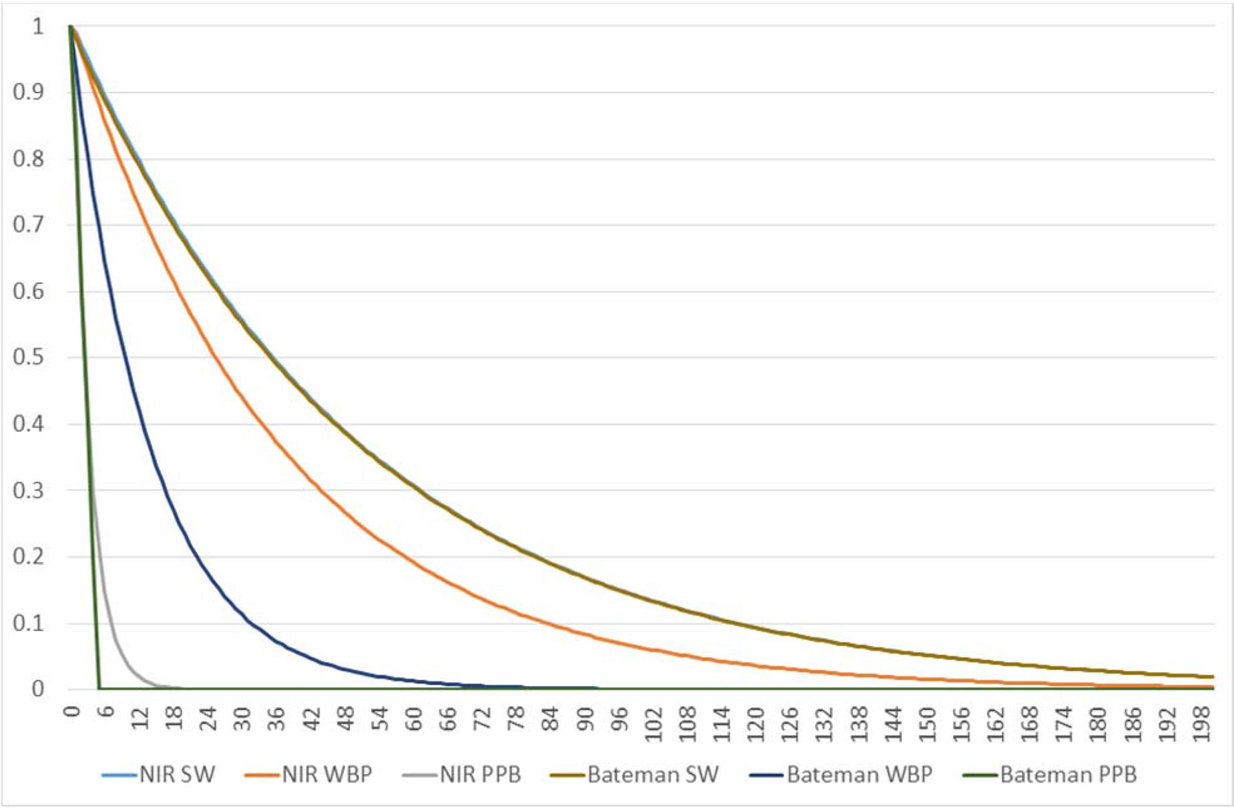
Harvested Wood Flow Carbon Liberation Curves: Comparison of NIR (2018) (SW, WBP, PPB) with Bateman & Lovett (2000) (Bateman SW, Bateman WBP, Bateman PPB)
Tables
Agricultural Carbon Emission Factors and GHG equivalent conversions
| Energy CO 2 | Energy CH 4 | Energy CH 4 | CH 4 | Agri CH 4 | Total CO 2 | Total CO 2e | |
|---|---|---|---|---|---|---|---|
| tCO 2/€ | tCH 4/€ | tCO 2e/€ | tCH 4/head/yr | tCH 4/head/yr | tCO 2e/head | tCO 2e/LU | |
| Dairy | 0.124 | 0.00012 | 3.129 | 3.129 | |||
| Cattle | 0.051 | 0.00013 | 1.308 | 2.975 | |||
| Sheep | 0.006 | 0.00001 | 0.152 | 0.684 | |||
| Horses | 0.020 | 0.00015 | 0.544 | 1.238 | |||
| Pigs | 0.006 | 0.00003 | 0.262 | 1.176 | |||
| Poultry | 0.000 | 0.000001 | 0.00590 | 0.006 | |||
| Fuel | 0.003 | 0.00000154 | 0.00000015 | ||||
| Fertiliser | 0.000032 | ||||||
| Crops | 0.00000041 | ||||||
| CO 2 equiv conversion factor | 1 | 25 | 298 | 25 | 298 |
-
Source: Common Reporting Framework 2015[6]
Private Returns to Planting SS Forest in 2015 (annual equivalised (AE) of Average NPV per ha) at 5% discount rate
| Yield Class | Average AE of NPV (€ ) |
|---|---|
| 24 | 563 |
| 20 | 473 |
| 18 | 425 |
| 14 | 355 |
-
Source: C-ForBES
-
Carbon Models, Assumptions and Validation
Average Private Returns (Gross Margin € ha −1) to Agriculture by Soil Code and Farm System (2015)
| SC | YC | Specialist Dairy | Cattle Rearing | Cattle Other | Sheep | Tillage |
|---|---|---|---|---|---|---|
| 1 | 24 | 1566 | 1029 | 996 | 954 | 1098 |
| 2 | 24 | 1181 | 855 | 882 | 1066 | 1186 |
| 3 | 20 | 1145 | 766 | 764 | 740 | 1103 |
| 4 | 20 | 1082 | 656 | 878 | 859 | 803 |
| 5 | 18 | 670 | 497 | 550 | 471 | |
| 6 | 14 | 584 | 583 | 356 | 681 | |
| All | All | 1237 | 784 | 867 | 811 | 1114 |
-
Source: Teagasc NFS (2015)
-
Note: SC: Teagasc NFS Soil Code (1 – Best, 6 – Worst), YC: Forest Yield Class
Economic Components of Agriculture and Forestry (2015) (Annual Equivalised NPV per ha (€)
| Soil Code | Agriculture | Forestry | ||
|---|---|---|---|---|
| Mkt Gross Margin /ha (A) | Subisides /ha (B) | Mkt Gross Margin /ha (©) | Subsidies /ha (D) | |
| € | € | € | € | |
| SC1/YC24 | 1200 | 366 | 224 | 306 |
| SC2/YC22 | 792 | 388 | 224 | 306 |
| SC3/YC20 | 803 | 342 | 154 | 302 |
| SC4/YC18 | 731 | 351 | 154 | 302 |
| SC5/YC16 | 356 | 314 | 124 | 300 |
| SC6/YC14 | 258 | 326 | 52 | 298 |
| Average | 878 | 359 | 155 | 296 |
Average Annual Equivalised Social Return to Planting one hectare of Unthinned Forest (2015) Displacing Agriculture
| Soil Code | Private Return10 | Agriculture | Forestry | Social Return | |||
|---|---|---|---|---|---|---|---|
| (C+D) – (A+B) (€/ha) | E11 | F12 | C – (A+B) + (F-E)*P13 (€/ha) | ||||
| tCO 2 Value (P) | €0 | tCO 2 | tCO 2 | €20 | €32 | €100 | €163 |
| SC1 | 1036 | -9.2 | 14.9 | -556 | -268 | 1365 | 2878 |
| SC2 | 651 | -8.4 | 14.9 | -185 | 95 | 1680 | 3148 |
| SC3 | 690 | -7.5 | 11.8 | -304 | -72 | 1239 | 2455 |
| SC4 | 627 | -7.4 | 11.8 | -242 | -11 | 1298 | 2511 |
| SC5 | 246 | -4.5 | 10.8 | 59 | 242 | 1281 | 2243 |
| SC6 | 234 | -4.9 | 7.8 | 19 | 171 | 1031 | 1828 |
| Total | -8.0 | 13.4 | -359 | -103 | 1347 | 2691 | |
-
Note: No-thinning assumed; BEF Factors from the 2015/18 National Inventory Reports are used;
-
All values are discounted using a 5% discount rate. Sensitivity Analyses
Comparing the Annual Equivalised tCO 2 for Thinned Forests by Soil Type if all thinnings are used for energy
| Soil Code | Equal Allocation from Thinnings and Clearfell to Energy | Thinnings only Allocated to Energy |
|---|---|---|
| 1 | 10.77 | 9.60 |
| 2 | 10.77 | 9.60 |
| 3 | 9.04 | 8.16 |
| 4 | 9.04 | 8.16 |
| 5 | 9.14 | 8.37 |
| 6 | 5.37 | 4.83 |
| Average | 9.98 | 8.95 |
-
Note: 2015/18 National Inventory Report Assumptions
Total Annual Equivalised tCO 2 Forest Carbon Sequestration for Mineral and Peat Soils by Yield Class
| Yield Class | Mineral | Peat |
|---|---|---|
| 24 | 12.69 | 10.56 |
| 24 | 12.69 | 10.56 |
| 20 | 10.44 | 8.32 |
| 20 | 10.44 | 8.32 |
| 18 | 9.34 | 7.21 |
| 14 | 7.60 | 5.48 |
| Average | 11.56 | 9.43 |
-
Note: For simplicity purposes in peat calculations, these values are calculated using EFs from NIR (2012)
Share of Farms with greater social returns from Forestry than from Agriculture (Annual Equivalised NPV-2015) for a range of Discount Rates
| Discount Rate | 0 | 1 | 2 | 3 | 4 | 5 | 6 | 7 |
|---|---|---|---|---|---|---|---|---|
| Carbon Value (€): | 32 | |||||||
| Soil Code | ||||||||
| 1 | 1.000 | 0.998 | 0.958 | 0.846 | 0.720 | 0.643 | 0.597 | 0.563 |
| 2 | 1.000 | 1.000 | 0.991 | 0.940 | 0.923 | 0.895 | 0.853 | 0.824 |
| 3 | 1.000 | 1.000 | 0.955 | 0.868 | 0.805 | 0.755 | 0.736 | 0.724 |
| 4 | 1.000 | 1.000 | 0.969 | 0.922 | 0.844 | 0.814 | 0.779 | 0.741 |
| 5 | 1.000 | 1.000 | 0.979 | 0.932 | 0.919 | 0.912 | 0.912 | 0.903 |
| 6 | 1.000 | 1.000 | 1.000 | 1.000 | 1.000 | 1.000 | 1.000 | 1.000 |
| Total | 1.000 | 0.999 | 0.969 | 0.892 | 0.820 | 0.774 | 0.739 | 0.712 |
-
Distribution of Private and Social Returns
Share of Farms with a positive Private and Social return to Forestry by BEF Assumption and inclusion of Forest Subsidy
| Private Return | Social Return | ||||
|---|---|---|---|---|---|
| Carbon value (€) | 0 | 20 | 32 | 100 | 163 |
| BEF (NIR, 2012) | |||||
| Incl Farm Subsidy | 0.324 | 0.264 | 0.427 | 0.943 | 0.998 |
| Excl Farm Subsidy | 0.551 | 0.577 | 0.672 | 0.983 | 0.999 |
| BEF (NIR, 2015) | |||||
| Incl Farm Subsidy | 0.324 | 0.304 | 0.466 | 0.965 | 0.999 |
| Excl Farm Subsidy | 0.551 | 0.594 | 0.697 | 0.991 | 0.999 |
-
Impact of substitution of trees for livestock
Area of livestock production that could be offset by one hectare of SS, at different livestock densities (LUha−1), with/without accounting for land use change (LUC) by soil code
| Soil Code | Stocking Rate | Area (ha)offlivestock displaced by one ha of forest | Area (ha) of livestock displaced by one ha of forest | LU displaced per Ha of Forest | LU displaced per ha of Forest | LU per Ha of Forest |
|---|---|---|---|---|---|---|
| LU per Ha | No LUC (not accounting for displaced emissions) | With LUC (accounting for displaced emissions) | No LUC | With LUC(No Thin) | With LUC (Thin) | |
| 1 | 1.57 | 1.62 | 2.62 | 2.56 | 4.13 | 3.03 |
| 2 | 1.52 | 1.76 | 2.76 | 2.67 | 4.18 | 3.03 |
| 3 | 1.33 | 1.59 | 2.59 | 2.12 | 3.45 | 2.69 |
| 4 | 1.36 | 1.59 | 2.59 | 2.17 | 3.52 | 2.75 |
| 5 | 0.87 | 2.38 | 3.38 | 2.06 | 2.93 | 2.29 |
| 6 | 0.90 | 1.61 | 2.61 | 1.44 | 2.34 | 1.85 |
| Average | 1.41 | 1.68 | 2.68 | 2.38 | 3.79 | 2.84 |
Enteric Fermentation and Nitrous Oxide Emission Factors
| CH 4 | N 2 O | ||
|---|---|---|---|
| Enteric Fermentation | Manure Management | Manure Management (kt) | |
| Emission Factor | (kg/head CH 4/yr) | (kg CH 4/head/yr) | (kg/N 2 O/head) |
| Dairy | 113.41 | 10.30 | 0.12 |
| Cattle | 46.39 | 4.43 | 0.13 |
| Sheep | 5.61 | 0.39 | 0.01 |
| Horses | 18.00 | 1.99 | 0.15 |
| Pigs | 1.33 | 5.04 | 0.03 |
| Poultry | 0.00 | 0.22 | 0.00 |
| Deer and Goats | 25.00 | 1.62 | 0.12 |
-
Source: Common Reporting Framework http://www.epa.ie/pubs/reports/air/airemissions/ghg/nir2015/
Average LU per Ha by Soil Code
| Soil Code | Dairy | Cattle | Sheep |
|---|---|---|---|
| SC1 | 2.09 | 1.74 | 1.62 |
| SC2 | 2.03 | 1.48 | 2.13 |
| SC3 | 2.00 | 1.42 | 1.66 |
| SC4 | 1.84 | 1.35 | 1.25 |
| SC5 | 1.58 | 0.73 | 0.42 |
| SC6 | 1.14 | 1.69 | |
| Average | 2.00 | 1.45 | 1.28 |
-
Source: C-ForBES
Average tCO2 per hectare by source of emissions by Soil Code
| Soil Code | Dairy | Cattle | Sheep | Fuel | Fertiliser | Crops |
|---|---|---|---|---|---|---|
| SC1 | 1.77 | 4.00 | 0.21 | 0.000207 | 0.001297 | 0.000019 |
| SC2 | 0.96 | 4.00 | 0.79 | 0.000190 | 0.001071 | 0.000018 |
| SC3 | 1.15 | 3.79 | 0.56 | 0.000221 | 0.000937 | 0.000008 |
| SC4 | 1.31 | 3.58 | 0.38 | 0.000219 | 0.000853 | 0.000003 |
| SC5 | 0.36 | 1.42 | 0.41 | 0.000080 | 0.000303 | 0.000002 |
| SC6 | 0.00 | 2.80 | 0.68 | 0.000107 | 0.000378 | 0.000001 |
| Average | 1.24 | 3.57 | 0.45 | 0.000191 | 0.000993 | 0.000012 |
-
Source: C-ForBES
C-ForBES Modelling Assumptions
| Model component | C-ForBES parameters and assumptions | Comparisons with parameters/assumptions in NIR (2018) and Bateman and Lovett (2000) | Additional notes |
|---|---|---|---|
| Scale of analysis | Per hectare net carbon storage or emissions in a given year. | Bateman and Lovett (2000): Per hectare net carbon storage or emissions in one year.NIR (2018): National Carbon Stock Change (CSC) over time. | |
| Period of analysis | 200 years. To accommodate approx. 4 rotations of SS (dep on YC) to allow for consideration of half-life of Harvested Wood Products (HWP). Replanting is assumed in the year following harvest. | Bateman and Lovett (2000) model extends to 1000 yearsNIR (2018): Annual CSC 1990 – 2016 | |
| Yield Class (YC) | Yield classes14-24 are analysed. YC14 is lower bound for eligibility for afforestation grants and subsidies. | NIR (2018) reports across all historic and current YCs.Bateman and Lovett (2000) estimate YC 6 – 24. | |
| [1] C-ForBES Forest ManagementAssumptions derived from Teagasc FIVE (see Ryan et al., 2018) | [1a] Tree species:Forest Investment and Valuation Estimator (FIVE):Sitka spruce (SS), which is the most commonly planted conifer in Ireland.To reduce complexity a simplifying assumption is made to model one hectare of pure SS (see [2] and [11]) as cost, growth and price data in FIVE are not as robust for mixtures of broadleaf and conifers.However, productive area is modelled at 85% to account for broadleaf component. In this analysis therefore, carbon sequestration from broadleaves is not modelled. | NIR (2018) estimates CSC for all species planted in Ireland.Bateman and Lovett (2000) model and map C storage for SS and Beech in Wales | “The forest must contain a minimum of 15% broadleaves by area. This can comprise: broadleaves planted in broadleaf GPC plots of minimum width; and/or broadleaves planted as part of the 'at least 10% diverse' requirement for GPC 3; and/or additional broadleaves planted for environmental and landscape reasons”.www.teagasc.ie/forestry/Grants |
| [1b] Forest Yield:Merchantable Timber Volume (MTV)(Edwards and Christie, 1981) | NIR (2018) is based on a range of models including FORCARB (based on Edwards and Christie, 1981), CARBWARE & Carbon Budget Model (CBM) (NIR, 2019).Bateman and Lovett (2000): MTV from (Edwards and Christie, 1981) and combine with data on carbon storage in Sitka spruce (Cannell and Cape, 1991) to plot thin and no-thin carbon storage curves. | ||
| [1c] Thinning:Marginal Thinning Intensity (MTI)15 @5 year intervals from Edwards and Christie (1981) | NIR (2018)/Bateman and Lovett (2000) also use this static thinning assumption. | ||
| [1d] Rotation:‘Reduced rotation’ = (Age of max MAI – 20%)16 (Phillips, 1998; Anon, 1977, ). | NIR (2018)rotation = max MAI from CARBWARE (Black, 2016).Bateman and Lovett (2000) estimates felling year (F) based on age of max NPV for given species, YC and discount rate – see Bateman (1996) | ||
| [2] ForSubs model (Ryan et al. (2016) | Forest subsidy:General Planting Category GPC3 (10% Diverse Conifer, e.g. Sitka spruce and 10% broadleaves)€510/ha/year - paid annually for 15 years for first rotation only | GPC 3 – 10% Diverse Conifer/Broadleaf:Comprises of a mix of Sitka Spruce/Lodgepole pine together with at least 10% Diverse conifer (approved conifer other than SS/LP). Broadleaves adjacent to roads and watercourses may also form part of this 10% www.teagasc.ie/forestry/grants | |
| [3] CostsTeagasc FIVE (Ryan et al., 2018) | Ground preparation, fencing, planting, maintenance, insurance, replanting. | ||
| [4] Timber prices | Coillte (State forestry body) 10 year average timber pricesAnnual timber price series published annually by Irish Timber Growers Association (ITGA) (see Symons et al. (1994); Teagasc (2019)) | ||
| [5] NPV discount rate | The conventional discount rate used for forestry in Ireland is 5% (Clinch, 1999). | Bateman and Lovett (2000) also use a discount rate of 5% for forest NPVs. | |
| [6] Soil organic matter (SOM) | Analysis assumes land use change on grassland on mineral soil only with no change in SOC.In the sensitivity analysis of planting on mineral or peat soils, the coefficients from NIR (2012) are used. | NIR (2018) assumes (a) no carbon stock change on the planting of forests on mineral soils and (b) a mean organic soil EF of 0.59 t C/ha/year over the first rotation (50 years) as organic soils are not a source following successive rotations (Byrne and Farrell, 2005).Bateman and Lovett (2000) assume long term net gain of soil carbon (50 t C ha-1 on mineral soils) or loss (750 t C ha-1 on peat soils) occurring within 200 years. | NIR (2018) categorises Irish soils into three major groupings based on soil carbon characteristics. All mineral soils are grouped together, while all organic soils with an organic layer greater than 30 cm are classified as peat. Finally, organic soils with an organic layer less than 30 cm are classified as peaty/mineral.CARBINE (Temperli et al., 2020): V Changes in soil carbon are assumed to take place in response to land use change. Magnitude and changes over time are estimated according to soil type (texture) and major land use category. |
| [7] Early growth | We use a logistic function to interpolate early growth and the growth in 5 year intervals recorded in Edwards and Christie (1981) models. | NIR (2018) uses a modified expo-linear growth function (Monteith, 2002) to simulate early annual growth.Bateman and Lovett (2000) fitted an S shaped curve to Edwards and Christie (1981) data | |
| Carbon mass of Sitka spruce (SS) | [8] Basic density 0.387 (NIR, 2012, p. 123 ) | [9] Carbon fraction 0.5 (NIR, 2015, p. 123 ) | |
| Biomass – above ground | [10] Biomas Expansion Factor (BEF) follows NIR (2018) methodology. | NIR (2015). A dynamic BEF is used in this analysis based on species, yield class and growth phase. Ranging from a value of 2 to 1.68 for lower YCs (14 & 16), 3 to 1.68 for YCs 18 & 20, 4 to 1.68 for the most productive YCs (22 & 24). A constant BEF of 1.68 is utilised once stand volume is equal to or greater than 200m 3 ha− 1 Bateman and Lovett (2000).estimated functional relationships for livewood. MTV is related to total woody volume (TWV) by allowing for branchwood, roots, etc. (Corbyn et al., 1988). | NIR (2018): Based on the model developed by Dewar and Cannell (1992), (Kilbride et al., 1999) used a static value of 1.3 for all species, age and yield classes, while the 2012 NIR uses a value of 1.64. However, since the allocation of biomass between different forest components is dependent on species, yield class and the growth phase of the forest, current estimates of sink capacity have been revised to use age and species-specific BEF values that include the below ground fraction. |
| [11] Productive area | 85% of the area taken out of agriculture is classified as productive area due to mandatory areas of biodiversity enhancement (ABE), set-back distances for roads, rivers, houses, fencing, unplantable terrain etc., (Ryan et al., 2018). | In scaling up, NIR (2018) applies a 10% area reduction to account for open spaces. | |
| Biomass – below ground | [12] Ratio of below ground to above ground biomass: 0.2Country specific ratio (NIR, 2015) | ||
| DOM | Litter [13 ] LLF represents the transfer of carbon from the above ground pool to the litter pool. It is simulated using derived leaf/needle biomass (LB) and the foliage turnover rates (Ft) from Thorne and Fingleton (2006):LLF = LB × F t The F t rate is assumed to be 6.7 years for conifer crops and 1 year for broadleaf crops (Thorne and Fingleton, 2006). Needle biomass is calculated according to the equation defined in Annex 3.4.A.4 of NIR (2018):LB = 0.025 × AB + 0.089 × exp (−0.003 × AB)The litterfall LLF is assumed to decompose at a rate of 14% per year (NIR (2018) p 222). | NIR, 2018 – p197: Biomass carbon losses from the above ground biomass pool are calculated based on harvest (Ltimber), harvest residue (LHR), litter fall (LLF), above ground losses due to mortality (Lmort(AB)) and fire (Lfire):Ltimber is calculated based on the above ground biomass removed from harvest,LHR includes the harvest residue representing all stems and branches with a DBH less than 7cm and litter left on site after timber is removedLLF reflects the transfer of carbon from the AB pool to the litter poolNIR (2018): Equation from NIR (Thorne and Fingleton, 2006) (needle turn- over is 6.7 years for conifers and annually for broadleavesCalculation of matter from equation in NIR, 2018Decomposition = 14% decline/yr p222 NIR, 2018 Bateman and Lovett (2000): litter is not modelled | CARBINE (Temperli et al., 2020): Litter is not modelled |
| Deadwood [14]Inflow is 1.6%Decomposition rate is 14% decline /year (Carbware) | NIR (2018) Mortality:Growth, harvest and mortality derived from Edwards and Christie (1981) described by Black et al. (2012).Net deadwood stock changes (CDW) are derived from carbon inputs associated with timber extraction residue (Ltr), timber from mortality (Mtimber), dead roots from mortality (Lmort(BB)), roots from harvest (LHRroot) and carbon loss due to decomposition of the new and previously existing deadwood pool (DDW):Biomass carbon losses from the below ground biomass pool are calculated as the sum of losses due to death of roots after harvest (LHRroot), natural mortality of roots (Lmort(BB)) and root death following fire (Lfire).Bateman and Lovett (2000): Assume 5 year oxidation of deadwood | ||
| [15] Harvest losses | We assume differential harvest losses for each harvest as per Teagasc FIVE.Ist Thin – 14% loss of Merchantable Timber Volume (MTV)2nd Thin - 12% loss of MTVSubsequent Thin - 9%Clearfell/Final harvest – 5% | NIR (2018) assumes static harvest losses of 4% | Morison et al. (2012) include HL in HWP as they may not be immediately oxidised |
| Wood fuel oxidation [16] | 34%In the 2017 Wood Flow report, 34% of forest biomass is used as wood fuel (Knaggs and O’Driscoll, 2017). | ||
| HWP allocations [17] | ForBES follows Pingoud & Wagner (2006) model (2006 IPCC guidelines)Assumes the same allocation of wood to the value chain from thinnings and from final harvest (scenario analysis to examine alternative scenario).Allocation of SW, WBP and PPB to HWPSW: 52%, WBP 48%.PPB: zero (no longer any paper production). | Phimmavong and Keenan (2020) model (2006 IPCC guidelines) | The UK CARBINE model (Temperli et al., 2020) allocates MTV to HWP pool (long-lived sawnwood, short-lived sawnwood, particleboard and paper), with remainder to waste. |
| Saw-milling losses [18] | SW: 50%WBP: 41% | ||
| IPCC conversion factor [19] | Conversion factor from C to CO 2: 3.67 | 3.67 | A cost of USD 1 per tonne of carbon dioxide is equivalent to a cost of USD 3.67 per tonne of carbon. OECD |
| Carbon Valuation [20] | Carbon values applied as per Irish Government shadow price of carbon for 2019, 2020, 2030, 2040.Future carbon sequestration and emissions are discounted at 5%. | NIR (2018) does not discount future carbon sequestration or emissions.Bateman and Lovett (2000) discount carbon at 5% and include scenario analysis for discount rates of 2 – 12% | |
| Annual Equivalised (AE) NPV per hectare [21] | Assume no agricultural income in year of planting |
Harvested Wood Flow Carbon Liberation Curves: Comparison of NIR (2018) (SW, WBP, PPB) with Bateman & Lovett (2000) (Bateman SW, Bateman WBP, Bateman PPB)
| Bateman | 0 | 0 | 0 | 1 |
|---|---|---|---|---|
| Harvest Loss | 0 | 1 | 1 | 0 |
| Energy | 0 | 0 | 1 | 0 |
| Sawnwood (SW) | 0.255 | 0.242 | 0.160 | 0.253 |
| Wood-based panels (WBP) | 0.186 | 0.177 | 0.117 | 0.072 |
| Paper and paper board (PPB) | 0.020 | 0.019 | 0.012 | 0.015 |
Comparing the Annual Equivalised tCO2 for Thin and No Thin by Soil Code/Yield Class for 2012 and 2015/18 Biomass Expansion Factor (BEF) National Inventory Report Assumptions
| Soil Code (SC)/Yield Class (YC) | 2012 BEF | 2015/18 BEF | Ratio | 2012 BEF | 2015/18 BEF | Ratio |
|---|---|---|---|---|---|---|
| No Thin | No Thin | No Thin | Thin | Thin | Thin | |
| SC1/YC24 | 12.69 | 14.86 | 1.17 | 8.46 | 10.77 | 1.27 |
| SC2YC/24 | 12.69 | 14.86 | 1.17 | 8.46 | 10.77 | 1.27 |
| SC3/YC20 | 10.44 | 11.83 | 1.13 | 7.58 | 9.04 | 1.19 |
| SC4/YC20 | 10.44 | 11.83 | 1.13 | 7.58 | 9.04 | 1.19 |
| SC5/YC18 | 9.34 | 10.75 | 1.15 | 7.43 | 9.14 | 1.23 |
| SC6/YC14 | 7.60 | 7.80 | 1.03 | 5.14 | 5.37 | 1.04 |
| Average | 11.56 | 13.37 | 1.16 | 8.04 | 9.98 | 1.24 |
-
Note BEF – Biomass expansion Factor
Data and code availability
The data used in this model is publicly available. The farm level data (National Farm Survey) is accessible via the Irish Social Science Data Archive, while the growth curves used in the model are available online in the referenced documentation. All other parameters used in the model have been documented in the extensive documentation provided within this and referenced papers.
The models have been coded in Stata. While they are not currently stored in the public domain (primarily because they haven’t been documented to a standard to facilitate such dissemination), we are happy to share code for the algorithms and indeed have documented the main algorithms and modelling choices made in this paper and other cited references.