Investigating the Incidence of Value Added Tax on Households Income: New Evidence from Italy
- Ministry of Economy and Finance, Department of Finance, Italy
- Article
- Figures and data
- Jump to
Abstract
This paper analyses the incidence of the Value Added Tax (VAT) on Italian households income. To address this question, we developed a non-behavioural microsimulation model, the Value Added Tax Simulation Model (VATSIM-DF II). The goals of VATSIM-DF (II) are to estimate actual and expected VAT revenues, assess the VAT incidence on households disposable income, and simulate the distributional effects of changes in fiscal policies in Italy. Compared to existing models, the main achievements of this study are: (i) the creation of a unique original dataset, which includes tax register data; (ii) the implementation of a matching procedure, based on Tax Register data, which outperforms other data fusion strategies used in the existing literature. These innovations allow us to create a reliable and unique dataset to simulate changes in VAT and to produce results consistent with the most updated macroeconomic data. We tested our model, at current VAT legislation, and we show the VAT burden on Italian households confirming the regressivity of VAT. Finally, we analyse the effect of a revenue neutral reform, with two VAT rates, which applies the reduced VAT rate also to female and babies sanitary products.
1. Introduction
Since the introduction of the Value Added Tax in Italy, in 1973, VAT rates were subject to a number of changes and the recent debate on tax-shift from direct to indirect taxation revamped the attention on this topic and the need to rigorously assess the effects produced by fiscal policies changes. To this end, along the years, researchers and institutions developed different instruments to assess the economic effects produced by variations in VAT rates. In particular, microsimulation models were proven to be powerful tools to predict the economic effects of fiscal changes for governments, firms and households. In Italy, there exist several microsimulation models on VAT and the objective of this paper is to contribute to the existing literature by proposing a new non-behavioural distributional model, the Value Added Tax Simulation Model (VATSIM-DF II).
The goals of VATSIM-DF (II) are: (i) to estimate actual and expected VAT amounts; (ii) to estimate the VAT incidence on households’ disposable income; (iii) and to simulate the distributional effects of changes in fiscal policies. The idea to develop VATSIM-DF (II) origins from the need to produce an original model to check the distributional effects of VAT and to support Italian policy makers in designing fiscal policies. Compared to existing models, the main achievements of this study are the creation of a unique original dataset, which includes Tax Register data, and the implementation of a matching procedure, which outperforms other data fusion strategies used in the existing literature. Our model has the great advantage to benefit from several data sources that are not accessible by all research institutions.
Our model contributes to a rich literature that, along the years, proposed powerful microsimulation models on the Italian VAT, which contributed to shed a light on this topic. One of the first works in Italy was due to Marenzi (1989) who, relying on the SHIW (Survey on Household Income and Wealth) data, simulated the distributional effect of taxation in Italy. Then, in 1999, the Microsimulation Unit in the Department of Applied Economics at the University of Cambridge, 1 launched Euromod, a tax-benefit tool which covers 15 European countries, including Italy, that was then updated in 2017 with the creation of Euromod-ITT (Bourguignon et al., 1997; Immervoll et al., 1999; De Agostini et al., 2017; Ceriani et al., 2017). In 2001, Baldini published a study about MAPP98, a static tax-benefit microsimulation model, based on SHIW and consumption data, which was then updated in 2009, by Baldini and Pacifico, to assess the dynamic effects of changes in personal income taxes in the labour market (Baldini, 2000, Baldini and Pacifico, 2009). In 2007, the Department of the Treasury, at the Italian Ministry of Economy and Finance, developed the ITaxSIM (Italian TAXation SImulation Model) which relies on SILC data (Statistics on Income and Living Conditions) and focuses on the analysis of personal income tax, VAT, property tax, in-kind benefits and family allowances. 2 More recently, Arachi et al. (2012) and Gastaldi et al. (2014) built their microsimulation models to assess the effect of a shift from personal and corporate income taxes to indirect taxation. In particular, Gastaldi et al. (2014) rely on an integrated dataset, produced by Pisano and Tedeschi (2014) for their model (EGaLiTe). While Arachi et al. (2012) updated a microsimulation model originally developed by Pellegrino et al. (2010) to study the distributive impact of housing taxation in Italy. Another Italian micro-simulation tool is the BIMic model, developed by Curci et al. (2017) at the Bank of Italy. BIMic originally focused on the budgetary impact and on the distributional effects of social security contributions, family allowances, social benefits, personal income tax and property taxes. Recently, Curci and Savegnano (2019) extended the scope of BIMic by including the simulation of VAT to assess the effects of tax shifts from labour to consumption. Finally, at regional level, Maitino et al. (2013) developed the MicroReg model, which is a static model aimed at assessing the effects of PIT and VAT.
The common challenge and limitation faced by researchers and institutions to develop these microsimulation models is the lack of a dataset, which includes detailed information on both income and consumption. Indeed, in Italy a dataset on income and consumption does not exist. To match data on income and consumption from different datasets, researchers rely on a third data source used as “bridge” dataset (to calculate estimated income or consumption) or they match similar households basing on socio-demographic variables only. These procedures show limitations related to the reliability of a matching based on socio-demographic variables only, and to the small sample size and accuracy of aggregate data on consumption of the “bridge” dataset. 3 To address these issues, we take advantage of our unique access to the Tax Register data of all the households surveyed in the expenditure and income surveys. Indeed, we create a unique dataset on VAT, income and consumption (VATIC dataset) that is a strong innovation with respect to existing dataset produced before. Indeed, instead of relying on estimated consumption or socio-demographic variables only, we use Tax Register income data to match, with a high level of precision, households in the income survey with similar households from the expenditure dataset.
The value added of VATSIM-DF (II), with respect to the existing models, are: (i) the creation of a unique dataset with data on income and consumption with a very high level of reliability, since the matching procedure relies on tax codes and Tax Register data; (ii) and the adjustment of survey data on income and consumption to National Accounts data at the year of the simulation, which makes our estimations on VAT coherent with the most updated macroeconomic data. To the best of our knowledge, there are not existing models in Italy with these features and this makes VATSIM-DF (II) a promising tool for reliable microsimulations about the distributional effects of VAT.
In our paper, we show how our matching procedure, to create the VATIC dataset, outperforms those used in other microsimulation models to match different data sources. Also, we analyse the current VAT burden on Italian households showing the regressivity of VAT. Finally, we show the distributional effects that a revenue neutral reform of the VAT system could produce on the Italian households. The reform sets two VAT rates and applies the reduced rate also to female sanitary towel and babies nappies.
The paper is structured as follows: in Section 2 we describe the data used in our model; in Section 3 we briefly illustrate the strategies used in the literature to integrate different Italian data sources, we describe our method, and we test the reliability of our procedure with respect to those used in the literature; in Section 4 we report the steps to estimate theoretical and actual VAT amounts and VAT incidence on individuals’ disposable income, and we show the simulation outputs for 2019 at current legislation; Section 5 describes a revenue neutral reform and the expected VAT burden for households; Section 6 concludes.
2. Data
In Italy, a database including detailed information on both income and consumption expenditures is not available. This is the main challenge faced by researchers and institutions when it comes to create a reliable and rigorous dataset for microsimulation models. We rely on three different data sources: Statistics on Income and Living Conditions (SILC), Household Budget Survey (HBS), and Tax Register data. Unfortunately, SILC includes data on income but not on expenditure, vice versa for HBS. 4 The access to Tax Register data constitutes one of the main advantages of our model because it allows us to match households from the other two surveys by relying on declared income variables. 5 In this paper, we describe the model for 2019, that is based on surveys data from 2017, which are then updated to 2019 statistics by relying on National Accounts data (details are provided in Section 4). Below we provide a description of each dataset, while in Section 3 we provide details about the integration of the different data sources. 6
2.1. Data on income
The IT-SILC survey includes cross-sectional data about income, social exclusion, and multidimensional poverty at household and individual level. Households are randomly selected from the 640 Italian municipalities. Data about income are collected only for individuals aged more than 16 years old and refers to the year before the interview, while data about social exclusion refers to the survey year. Indeed, we use IT-SILC 2018 which includes data on income for 2017. Currently, data are collected through both Computer Assisted Personal Interview (CAPI) and Computer Assisted Telephone Interview (CATI). IT-SILC 2018 sample includes 21,173 households and 45,761 individuals (among them, 39,969 are aged more than 16 years old) (Istat, 2018a).
2.2. Data on expenditure
The HBS collects monthly data about expenditure for goods and services devoted to households expenditures. The two-stages sampling strategy identifies, first, municipalities and then it randomly selects households. The survey includes expenditure voices that can be aggregated to obtain COICOP (Classification of Individual Consumption by Purpose) voices, to ensure international comparability, and socio-demographic households variables. Data are collected through both interviews and daily self-administered diaries. The VATSIM-DF (II) 2019 model relies on HBS 2017, which includes 16,946 households (Istat, 2018b). Below we provide details about the procedure used to process data on expenditure.
2.2.1. Expenditure data preparation
Expenditure data are converted from monthly to yearly data. For what concerns non-durable goods we convert monthly data by simply multiplying expenditure values by twelve months. Regarding durable goods, we identify two groups of items: (i) those with a survey reference period of twelve months (e.g. means of transport, large household appliances, utensils, etc.) which do not require any conversion; (ii) those with a survey reference period of three months (e.g. furniture, small household appliances, etc.) which require an imputation procedure. For durable goods with a survey reference period of three months we implement a rigorous method to avoid the overestimation or underestimation of expenditures.
Indeed, since the survey questions refer to the last three months, we cannot exclude the possibility that households who did not report the expenditure in this time span have incurred the expenditure during the preceding nine months of the year. At the same time, we cannot be sure that households who incurred the expenditure in the last three months have (or don’t have) done the same during other months of the year. To address this issue, we impute these durables expenditures as follows. First, we use a Probit model to calculate the probability of a household to have incurred in the expenditure of at least one of these durable goods, during the last three months, given a set of socio-demographic characteristics (total expenditure, age, household size, employment status and type of job, household type, residence region, number of sons by age group, number of women and men within the households). Now, households who could have consumed durables outside the survey reference period are identified. Second, through a regression model we estimate the amount of money that households, given their characteristics, could have devoted to buy durable goods. Third, we create a dummy variable equal to one when the predicted probability (calculated with the Probit model) to have consumed durable goods is positive and we sort households according to this probability. Finally, we impute to each household the yearly amount of expenditure they could have incurred in, by assigning them the regression estimated values plus a hypothetical value of expenditure referring to the nine months not tracked by the survey. This value, is not constant but, decreases jointly with the predicted probability of the household to have spent money for this group of durable goods. The imputation process stops when the average annual expenditure, calculated through this imputation, equalizes the average annual expenditure we could have obtained by simply multiplying quarterly expenditures by four. The great advantage of our procedure is that, by simply multiplying durables to obtain the yearly data we overestimate the expenditure for households who reported consumption and we obtain a huge standard deviation which does not reflect the standard deviation of the survey quarterly data. Conversely, using the imputation procedure we obtain a yearly data with a standard deviation similar to the original one and an average expenditure similar to the one calculated by multiplying the observed data. Now the expenditure is assigned, not only to households who declared it in the survey, but also to households who did not report durable goods consumption in the last three months but could have incurred the expenditure during the rest of the year. Once the total amount of durables expenditure has been imputed to these households, we should impute also the value of single expenditure items pertaining to this group of goods. Through a statistical matching, based on the Mahalanobis distance, and relying on the set of households characteristics mentioned before (namely, total expenditure, age, household size, employment status and type of job, household type, residence region, number of sons by age group, number of women and men within the households), we match each household with positive durables expenditures observed in the survey with the most similar household with positive durables expenditures not observed in the survey but imputed through the aforementioned procedure. To each household with the imputed aggregated value, we assign the monthly item expenditure value of the nearest neighbor household with observed values. Then we convert the items monthly expenditures to the year, by multiplying for the ratio between yearly aggregated values (obtained by the imputation process) and monthly observed aggregated values.
A similar procedure is implemented for another group of goods related to the clothing and footwear sectors, which have a survey reference period of one month. Indeed, households who did not report the consumption of these goods in the last month could have bought them in other periods of the year. Since this group of goods is characterized by a seasonality of expenditures, instead of multiplying the monthly expenditure value for twelve, we implement a similar procedure followed for durable goods of the second group. However, in this case, we estimate the expenditure for eight months and impute the expenditure for the remaining fours, according to the decreasing probability of consuming this group of goods.
2.3. Tax Register Data
The third source of data is the Italian Tax Register, which includes declared income and an individual identifier, created on the basis of the tax code. 7 For the VATSIM-DF (II) 2019 we rely on Tax Register data from 2017.
3. Creation of the integrated dataset: VATIC
In order to develop our model, we need a dataset which includes, for each family, detailed information on income sources and expenditure items. In Section 3.1, we describe the methods used by existing studies to integrate Italian data sources, while in Section 3.2 we show the procedure used in our model and its value added.
3.1. Review of existing methods to integrate different Italian databases
In Section 1, we mentioned the most important microsimulation models on the Italian fiscal policies. All the authors faced the issue to create a database which includes both data on income and expenditures by matching different data sources. In Italy, the main sources of data on income and consumption expenditures are SILC and HBS, respectively, but they surveyed different households. The SHIW dataset of the Bank of Italy is the only source which includes both data on income and aggregate data on consumption but variables on specific expenditures items are not available.
Existing studies use the following methods to integrate the Italian data sources on income and consumption: (i) estimation of income or consumption in the SHIW dataset and use of the estimated coefficient as key variable to match the two datasets on income and consumption (Giarda et al., 2015; Cammeraat and Crivelli, 2020); (ii) statistical matching or hot deck methods based on socio-demographic variables only (De Vincenti and Pollastri, 2004; Sisto, 2006; Donatiello et al., 2014); (iii) a combination of these two strategies (Taddei, 2012); (iv) the integration between SHIW and HBS relying on data on income (Pisano and Tedeschi, 2014; Curci and Savegnano, 2019) or between SHIW and SILC through data on consumption (Cifaldi and Neri, 2013).
These methods show strength and weaknesses. Theoretically, SHIW could be integrated with HBS to involve information on items expenditure. However, the sample size of SHIW is small compared to the one of SILC and HBS and this is not suitable for all research purposes. Also, according to Cifaldi and Neri (2013) the risk is to consider the data accuracy level consistent across all the SHIW survey items. They show that the survey is more accurate for data related to income than for those about consumption, and this could lead to misleading results about saving rates. For these reasons, in microsimulation models, often SHIW is used as “bridge” dataset between SILC and HBS. Also, in this case there are several procedures available. According to Baldini et al. (2015) a matching procedure based on the estimated consumption (using SHIW data) is more efficient than a simple matching based on the available common socio-demographic variables. Also, matching households by strata produces better results with respect to a matching without grouping observations (ibid.). Pisano and Tedeschi (2014) tested both Propensity Score Matching (based on nearest neighbor algorithm with replacement) and Mahalanobis metric matching (coupled with propensity score), and then they select the latter procedure as it performs better.
To the best of our knowledge, our model is the first one which is able to integrate HBS and SILC without relying on SHIW (to impute income or consumption) and without relying on socio-demographic variables only to match datasets. Indeed, we use the Tax register database as “bridge” dataset. In Table 1, we provide an overview of the databases integrated in a sample of existing studies.
Review of Existing Studies on Italian Datasets Integration
| Authors and Year | Data Sources | ||||
|---|---|---|---|---|---|
| HBS | SILC | SHIW | ISTATMultipurpose | Tax Register | |
| Sisto (2006) | • | • | |||
| Pisano and Tedeschi (2014) | • | • | |||
| Curci and Savegnano (2019) | • | • | |||
| De Vincenti and Pollastri (2004) | • | • | • | ||
| Cifaldi and Neri (2013) | • | • | |||
| Taddei (2012) | • | • | • | ||
| Maitino et al. (2013) | • | • | • | ||
| Giarda et al. (2015) | • | • | • | ||
| Baldini et al. (2015) | • | • | • | ||
| Cammeraat and Crivelli (2020) | • | • | • | ||
| Donatiello et al. (2014) | • | • | |||
| Centro Studi Confindustria (2019) | • | • | |||
| VATSIM-DF (II) | • | • | • |
-
Source: Authors elaboration.
One could argue that we could rely on the Tax Register income of HBS households as reference value to estimate VAT incidence. However, the Tax Register data may show some limitation. Indeed, the SILC survey total income values (inclusive of social contributions) are 30% higher with respect to the Tax Register income values of SILC and HBS households. This difference may be caused by: i) tax erosion, because there are several income sources that are not in the Tax Register data (for instance, income from financial capital or, partially, from real estate) and we would need other datasets to have a complete picture of all the households income sources; ii) tax evasion in declared income (in particular, for self-employed income). For these reasons, we decided to rely on SILC as reference value to compute VAT incidence, instead of using Tax register income. 8
3.2. Method
To create the dataset for our microsimulation, the first step is to match SILC and HBS datasets with Tax Register data. This process is feasible because we can access the tax codes (anonymized through the creation of a unique identifier) of households included in SILC, HBS, and the Tax Register. This allows an exact matching between SILC households and Tax Register households, and between HBS households and Tax Register households. After this step, for each household we have data on the declared income, which constitutes one of the key variables used to match SILC and HBS households.
Indeed, during the second step the objective is to match SILC and HBS families. As explained in the previous section, we cannot rely on an exact matching because the households interviewed by these surveys are not the same. For this purpose, we need to integrate them through a statistical matching based on observable common variables. There are several techniques to implement a statistical matching. One of the most used is the Propensity Score Matching, a method originally developed by Rosenbaum and Rubin (1983) to identify a reliable control group in the setting of quasi-experimental impact evaluations. However, this technique can be used also to identify similar observations in the context of data fusion and can be based on the Euclidean distance (calculated through the propensity score) or on the Mahalanobis metric distance. In our model, we use a Nearest Neighbor matching (with replacement) based on the Mahalanobis distance. 9
To implement the statistical matching, we need to select variables that are comparable across the databases. The common variables to HBS and SILC are those included in the Tax Register (namely, household total income, household taxable income, household land and buildings income, first-earner total income, first-earner taxable income, other income) and a set of socio-demographic variables (such as, household size, type of family, first-earner age, sex, type of occupation, and education level) that were recoded and harmonized to be comparable across the two surveys. In Table 2, we show descriptive statistics about the common variables in HBS and SILC and we compare the two survey samples through a t-test. The p-value indicates that the two groups, on average, are not significantly different in income but they are significantly different in all the socio-demographic variables.
Comparison between SILC and HBS Samples before Matching
| Mean in SILC | Mean in HBS | p-value for difference | 95% C.I. | ||
|---|---|---|---|---|---|
| Tax Register household total income | 31,474.26 | 31,375.21 | 0.795 | -648.206 | 846.317 |
| Tax Register household taxable income | 30,584.36 | 30,553.10 | 0.930 | -668.825 | 731.349 |
| Tax Register first-earner total income | 23,972.73 | 24,195.20 | 0.479 | -837.955 | 393.008 |
| Tax Register first-earner taxable income | 23,158.80 | 23,285.98 | 0.673 | -717.342 | 462.993 |
| Tax Register household land and buildings income | 1,641.48 | 1,592.43 | 0.463 | -81.94 | 180.034 |
| Tax Register other household income | 3,260.84 | 3,365.34 | 0.649 | -554.238 | 345.246 |
| First-earner age | 59.49 | 59.02 | 0.006 | 0.136 | 0.798 |
| First-earner sex | 0.59 | 0.60 | 0.002 | -0.026 | -0.006 |
| Household size | 2.16 | 2.32 | 0.000 | -0.186 | -0.137 |
| Number of children | 0.26 | 0.32 | 0.000 | -0.077 | -0.05 |
| First-earner occupation | |||||
| Employed | 0.52 | 0.49 | 0.000 | 0.032 | 0.032 |
| Unemployed | 0.03 | 0.05 | 0.000 | -0.03 | -0.022 |
| Homemaker | 0.04 | 0.08 | 0.000 | -0.041 | -0.032 |
| Retired | 0.38 | 0.36 | 0.000 | 0.017 | 0.036 |
| Student, unable to work or other | 0.03 | 0.02 | 0.000 | 0.012 | 0.019 |
| First-earner education level | |||||
| None | 0.04 | 0.04 | 0.002 | -0.01 | -0.002 |
| Primary education | 0.17 | 0.18 | 0.072 | -0.015 | 0.001 |
| Lower secondary education | 0.27 | 0.28 | 0.423 | -0.013 | 0.005 |
| Vocational education (2-3 years) | 0.07 | 0.08 | 0.326 | -0.008 | 0.003 |
| Upper secondary education | 0.29 | 0.27 | 0.000 | 0.013 | 0.031 |
| University bachelor’s degree | 0.13 | 0.14 | 0.000 | -0.024 | -0.01 |
| Post graduate education | 0.03 | 0.01 | 0.000 | 0.012 | 0.017 |
| Type of Family | |||||
| Single | 0.37 | 0.31 | 0.000 | 0.055 | 0.074 |
| Couple with no children | 0.21 | 0.24 | 0.000 | -0.038 | -0.021 |
| Couple with 1 child | 0.16 | 0.17 | 0.016 | -0.017 | -0.002 |
| Couple with 2 or more children | 0.12 | 0.17 | 0.000 | -0.063 | -0.049 |
| Other | 0.14 | 0.11 | 0.000 | 0.023 | 0.036 |
-
Source: Authors elaboration.
-
Notes: sample weights are not used for estimations.
After the identification of common variables, we stratify the HBS and SILC samples by the 20 Italian regions and then within each of them by 18 income quantiles, based on the household total declared income from the Tax Register data. We obtain 380 strata of observations plus an additional stratum for all households with a negative declared income. Now the objective is to find, for each SILC household, the most similar household in the HBS dataset, given a set of characteristics. To this purpose, within each stratum, we implement a Nearest Neighbor matching (with replacement) based on the Mahalanobis distance relying on the following covariates (listed in Table 2): household total income, household taxable income, household land and buildings income, first-earner total income, first-earner taxable income, other income, household size, type of family, first-earner age, sex, type of job, education level.
Thanks to the matching, for each household of the SILC dataset we can identify the most similar household in the HBS survey. Therefore, we can assign to the SILC household the expenditure variables of the paired household. It is worth mentioning that, the matching procedure allows for replacement, hence one HBS household can be matched with more than one SILC household. 10
Generally, when statistical matching is used for quasi-experiment impact evaluations, verifying the matching performance is very important to produce reliable results. Indeed, after the statistical matching, the two groups (the treated and the control group) should not show significant differences in the covariates. However, in this case, we use matching to integrate two different data sources therefore also other aspects must be considered. As described by Rässler (2004), when the statistical matching is used for data fusion, the most important objective after matching is to preserve original individual values, joint distributions, correlation structures, and marginal distributions.
Hence, in order to check the matching: (i) we compare the SILC and HSB observations on average and in each income decile to check whether they are significantly different; (ii) and we provide a graphical representation of the variables distribution before and after the matching to verify whether they are preserved.
To the best of our knowledge, the existing studies on Italian microsimulation model do not test whether the two survey groups are, on average, significantly different after the matching. We provide this information to have a complete overview of the sample, even though the preservation of variables distributions is the most important aspect to check in case of data fusion. In Table 3, we compare SILC and HBS matched observations in the variables used for the matching. We want to check whether the two groups, after the matching, are not significantly different, on average, in terms of income.
Comparison between SILC and HBS Samples after Matching
| Mean in SILC | Mean in HBS | p-value for difference | 95% C.I. | ||
|---|---|---|---|---|---|
| Tax Register household total income | 31,474.26 | 30,638.12 | 0.075 | -83.54 | 1,755.83 |
| Tax Register household taxable income | 30,584.36 | 30,178.54 | 0.360 | -463.892 | 1,275.54 |
| Tax Register first-earner total income | 23,972.73 | 23,783.18 | 0.595 | -508.693 | 887.787 |
| Tax Register first-earner taxable income | 23,158.80 | 23,201.90 | 0.900 | -717.76 | 631.569 |
| Tax Register household land and buildings income | 1,641.48 | 1,033.65 | 0.000 | 483.753 | 731.91 |
| Tax Register other household income | 3,260.84 | 1,501.07 | 0.000 | 1,363.42 | 2,156.12 |
| First-earner age | 59.49 | 60.67 | 0.000 | -1.672 | -0.676 |
| First-earner sex | 0.59 | 0.62 | 0.000 | -0.05 | -0.02 |
| Household size | 2.16 | 2.01 | 0.000 | 0.123 | 0.187 |
| Number of children | 0.26 | 0.22 | 0.000 | 0.029 | 0.059 |
| First-earner occupation | |||||
| Employed | 0.52 | 0.48 | 0.000 | 0.048 | 0.048 |
| Unemployed | 0.03 | 0.02 | 0.020 | 0.001 | 0.008 |
| Homemaker | 0.04 | 0.03 | 0.017 | 0.001 | 0.01 |
| Retired | 0.38 | 0.45 | 0.000 | -0.076 | -0.046 |
| Student, unable to work or other | 0.03 | 0.02 | 0.000 | 0.015 | 0.023 |
| First-earner education level | |||||
| None | 0.04 | 0.03 | 0.002 | 0.003 | 0.012 |
| Primary education | 0.17 | 0.20 | 0.000 | -0.043 | -0.018 |
| Lower secondary education | 0.27 | 0.29 | 0.009 | -0.032 | -0.004 |
| Vocational education (2-3 years) | 0.07 | 0.05 | 0.000 | 0.014 | 0.026 |
| Upper secondary education | 0.29 | 0.31 | 0.085 | -0.027 | 0.002 |
| University bachelor’s degree | 0.13 | 0.11 | 0.000 | 0.007 | 0.024 |
| Post graduate education | 0.03 | 0.01 | 0.000 | 0.015 | 0.021 |
| Type of Family | |||||
| Single | 0.37 | 0.41 | 0.000 | -0.058 | -0.027 |
| Couple with no children | 0.21 | 0.26 | 0.000 | -0.058 | -0.032 |
| Couple with 1 child | 0.16 | 0.15 | 0.012 | 0.003 | 0.023 |
| Couple with 2 or more children | 0.12 | 0.11 | 0.270 | -0.004 | 0.013 |
| Other | 0.14 | 0.07 | 0.000 | 0.063 | 0.077 |
-
Source: Authors elaboration.
-
Notes: sample weights are not used for estimations.
Indeed, the p-value for the difference between SILC and HBS for the most important income categories shows that the two samples are not significantly different on average in these variables. However, the two groups are still significantly different in several socio-demographic variables (first-earner age and sex, household size, type of job, education level and type of family) and this is in line with what we observed before the matching.
An explanation for this unchanged difference in socio-demographic variables can be found in the sample stratification, implemented in the first step of the matching procedure. On the one hand, the stratification of households by income quantiles, allows us to obtain a good matching in terms of income, on the other, the creation of very small sub-sample of observations with similar income reduces the possibility for each SILC observation to find a similar HBS household in terms of socio-demographic characteristics. While in the setting of impact evaluation this could impair the validity of the study, for the purpose of our model this difference does not represent a limitation.
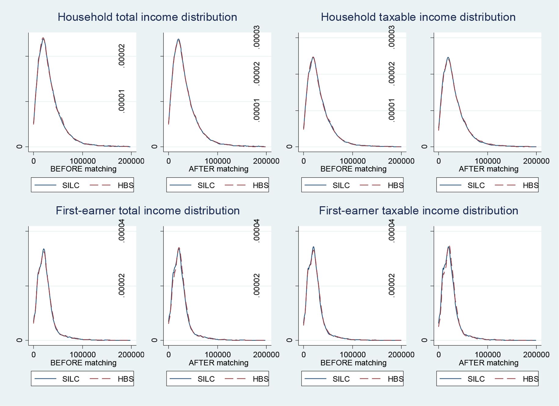
To further inspect the matching results, we compare the samples by the households total income deciles, that we are going to use to compute VAT incidence. Table 4 shows that households are not significantly different in each income decile except in the last one. This is due to the fact that in the SILC sample there are outliers with very high-income values, while in HBS sample there are not such extremely high values. While we can discard HBS observations who are not similar to SILC households, we cannot discard any SILC household because we need to keep the survey representative at the country level. Therefore, if there are SILC households that are very different from all the HBS observations, instead of discarding them, we compare them with the nearest HBS household even though it is not strictly similar. Finally, the most important aspect to be preserved after the matching are the variables distributions. In order to check whether distributions are preserved we show the Kernel density distribution of the most important income categories for SILC and HBS samples, before and after the matching (Figure 1).
Comparison between SILC and HBS Samples after Matching, by Income Deciles
| Average Household Total Income(Tax Register Data) | p-value for difference | 95% C.I. | |||
|---|---|---|---|---|---|
| SILC | HBS | ||||
| Decile 1 | 109.84 | 97.09 | 0.362 | -14.690 | 40.191 |
| Decile 2 | 6,123.82 | 6,100.1 | 0.853 | -227.601 | 275.042 |
| Decile 3 | 12,119.33 | 12,100.75 | 0.808 | -227.601 | 275.042 |
| Decile 4 | 17,048.14 | 17,003.47 | 0.479 | -79.197 | 168.543 |
| Decile 5 | 21,418.1 | 21,422.48 | 0.944 | -127.396 | 118.644 |
| Decile 6 | 26,253.72 | 26,184.46 | 0.337 | -72.261 | 210.775 |
| Decile 7 | 32,128.57 | 32,141.58 | 0.886 | -191.308 | 165.297 |
| Decile 8 | 40,270.44 | 40,385.72 | 0.382 | -373.659 | 143.105 |
| Decile 9 | 52,844.87 | 52,972.46 | 0.561 | -557.837 | 302.661 |
| Decile 10 | 100,286.9 | 92,542.72 | 0.000 | 3642.137 | 11,846.200 |
-
Source: Authors elaboration.

Tax Register Income Distribution Before and After Matching. Source: Authors elaboration based on Istat, 2018a Istat (2018a) and HBS 2017 data. Note: For graphical purposes, figures report the Kernel density distribution for income values below 200,000 Euros.
Before the matching the distribution represents all HBS household, while after the matching the distribution represents only HBS observations not discarded by the matching and it takes into account the fact that some observation is repeated more than once to be paired with SILC households. Figure 1 shows that the income distributions of SILC and HBS households is really similar with original samples and that this similarity is preserved even after the matching.
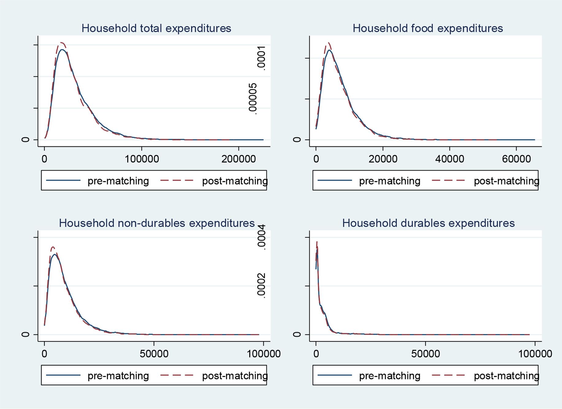
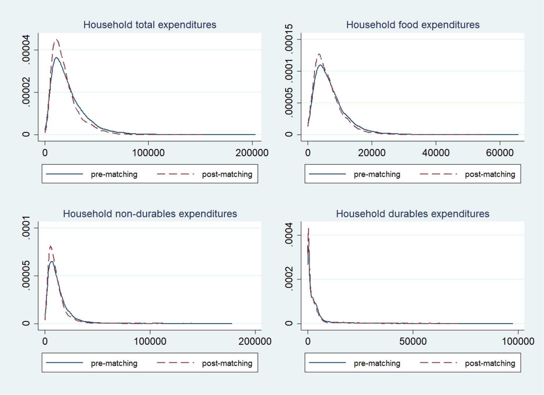
Additionally, we provide a graphic representation of the Kernel density distribution of expenditures, before and after the matching. We want to check whether the exclusion of some HBS household during the matching procedure could have altered the original distribution of the most important expenditure aggregates (namely: total expenditure, food expenditure, non-durable expenditures, durable expenditures). In Figure 2, we show that the two distributions are extremely similar before and after the matching.

HBS Households Expenditures Distribution Before and After Matching. Source: Authors elaboration based on HBS 2017 data. Note: Graphs report the Kernel density distribution of expenditures.
In general, we can consider the matching performance good for the purpose of our microsimulation model because the distributions are preserved, and the two groups, on average, are not significantly different in income.
Finally, we compared the performance of our matching with other two matching procedures commonly used by scholars. First, we tested a nearest neighbour matching with replacement (using the Mahalanobis distance) based on socio-demographic variables only and we stratify observations by type of job (as a proxy for income). After the matching, we compared the Tax Register declared income of the paired households and they are significantly different. Second, we replicate the most common procedure used in the literature, by matching SILC and HBS relying on the estimated consumption in the SHIW dataset. After the matching, we compare the Tax Register data of the two groups and we found that this procedure matches households that are significantly different in income. Also, the consumption distribution after matching is different from the consumption distribution observed before the matching (see Table A1). Basing on our estimations, the matching procedure used in this paper outperforms (thanks to the access to Tax Register data) those implemented in the existing literature.
4. The microsimulation model
Once we produced a reliable dataset, which includes both data on income and expenditures, we start to model the VAT microsimulation. In this section we describe the steps to estimate the expected and actual VAT amounts and the VAT incidence on households disposable income for the year 2019 with current legislation. We show how we compute the core microsimulation variables (Section 4.1) and then we describe the outputs of a microsimulation for 2019 with current VAT legislation (Section 4.2). Currently, the Italian VAT legislation establishes: (i) the application of a super reduced rate of 4% for basic food items, some medical services, books and newspapers; (ii) the application of two reduced rates of 5% and 10% for other food items and some house maintenance services; (iii) the application of the standard rate of 22% for other assets; (iv) the VAT exemption for some categories of goods or services, such as education. The same asset may be subject to different VAT rates (i.e. for heating gas a reduced rate of 10% is applied for domestic uses and up to a certain consumption threshold; in all other cases, the standard rate is 22%). Indeed, for each consumption item, we need to consider five weights, which represent the share of that item consumption subject to each VAT rate (4%, 5%, 10%, 22%, exempt).
4.1. The microsimulation core variables
As reported in Section 2, the last available survey data on income and consumption expenditures refer to 2017. To estimate VAT amounts and incidence coherent with the most updated National Accounts data, we convert 2017 survey data to 2019 National Accounts data. We cannot directly rely on National Accounts data on expenditure because this data is aggregated at national level and alone it is not suitable for a distributional analysis. However, we can use this data to convert expenditures from survey data to National Accounts data, as follows. First, we rely on 2019 National Accounts data on household expenditure (Aggregated into 12 consumption functions according to Coicop classification at 2 digits). (Istat, 2020a), and on the NIC Consumer Price Index weights (Classified with ECoicop at 5 digits) (Istat, 2020b). Weights are used to obtain the consumption for each product for the 12 Coicop consumption function. Then we estimate each good’s expenditure amount subject to each VAT rate by relying on the current VAT legislation (for more details see Calà et al., 2020). 11 Second, for each 2017 HBS good we calculate the aggregate expenditure for all households. Third, for each good and VAT rate, we calculate the relative change between the National Accounts expenditure data and the survey expenditure data. Since National Accounts data is not disaggregated at the household level, to obtain each household expenditure for 2019, we apply the aggregate relative change to each survey’s household expenditure. 12 Now, we know for every household, every good, and every VAT rate, the estimated expenditure in 2019. This data is perfectly consistent with the National Accounts aggregate data on expenditure, making our model ideal for microsimulation purposes and perfectly coherent with the macroeconomic data.
Expenditure data still include the VAT amounts paid by the household and VAT evasion. 13 Therefore, we calculate the net expenditure for each good, each VAT rate and each household. Once we have data on net expenditure, we can calculate the expected VAT revenues (namely, the VAT that should be paid by taxpayers when there is not evasion) by simply multiplying the net expenditure for the corresponding VAT rate. Then, to get data on VAT evasion for each item, we rely on the unobserved economy rates estimated by Istat (2020c). 14 The VAT taxable bases are calculated assuming that VAT gap for final consumption (business to customer - B2C) is entirely due to omitted invoicing. 15 Hence, we apply these evasion rates to the expected VAT revenue amount. Finally, we computed the actual VAT as the difference between the expected VAT and the VAT gap. Once we have all the data on VAT, we calculate actual expenditure as the sum between net expenditure and the actual VAT.
Now we can easily convert also income from survey data to National Accounts data, at the simulation year. First, we assign a positive income value to survey households with negative or null survey income values, by implementing an imputation process based on an OLS regression, which accounts for households expenditure and other socio-demographic characteristics. Second, we adjust data on income to equalize the National Accounts data on disposable income (estimated by Istat, 2020d). 16 To do so, we apply a procedure similar to the one implemented for expenditure data: we calculate the relative change at aggregate level (between survey and National Accounts data) and then we apply this variation to each household. 17 Finally, we have the VATIC dataset for 2019, which is consistent with National Accounts data, both on the consumption side and on the income side. 18
The model objectives are to assess the VAT incidence on households at current legislations and to simulate changes in VAT rates for a good or a set of goods. In case of simulations, we apply changes to VAT rates and to the relative amount of each good’s expenditure subject to the new rates.
4.2. Microsimulation outputs with current VAT legislation
In this section, we describe the VATSIM-DF (II) outputs. Figure 3 shows net consumption (that is the taxable VAT base) by household income deciles and VAT rates. We find that households in the first and tenth decile devote, respectively, around 8.6% and 5.8% of their total expenditure to goods with super reduced VAT rate (4%). While they spend, respectively, 33% and 35.1% of their total expenditure for goods with standard VAT rate (22%). For each VAT rate, we compute the expected and actual VAT revenue and the VAT gap (see Table 5). As expected, most of the VAT revenue is driven by goods with the standard VAT rate (22%) that are also those with the highest VAT gap in absolute terms.
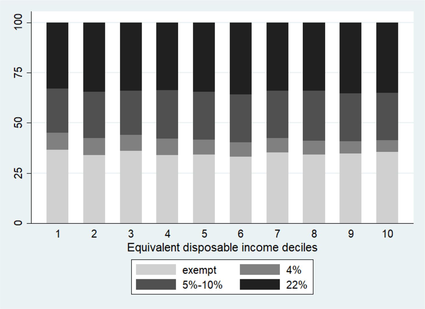
Net Consumption, by Households Income Deciles and VAT rates. Source: Authors elaboration.
Expected VAT, VAT Gap and Actual VAT, by VAT Rate
| VAT rate | Expected VAT | VAT Gap | Actual VAT |
|---|---|---|---|
| 4% | 2,909,905,600 | 307,970,616 | 2,601,934,984 |
| 5% | 114,201,667 | 17,058,621 | 97,143,046 |
| 10% | 23,543,919,955 | 3,817,302,226 | 19,726,617,733 |
| 22% | 76,787,961,011 | 8,186,778,456 | 68,601,182,579 |
| Total | 103,355,988,233 | 12,329,109,919 | 91,026,878,342 |
-
Source: Authors elaboration.
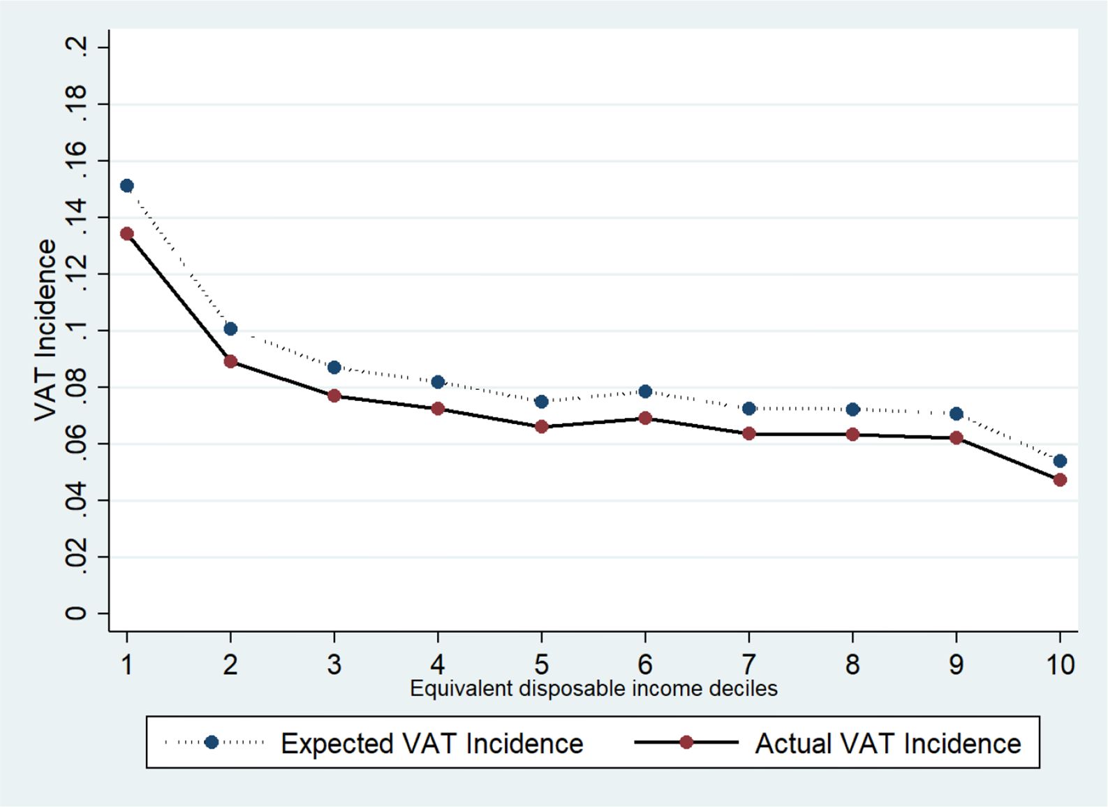
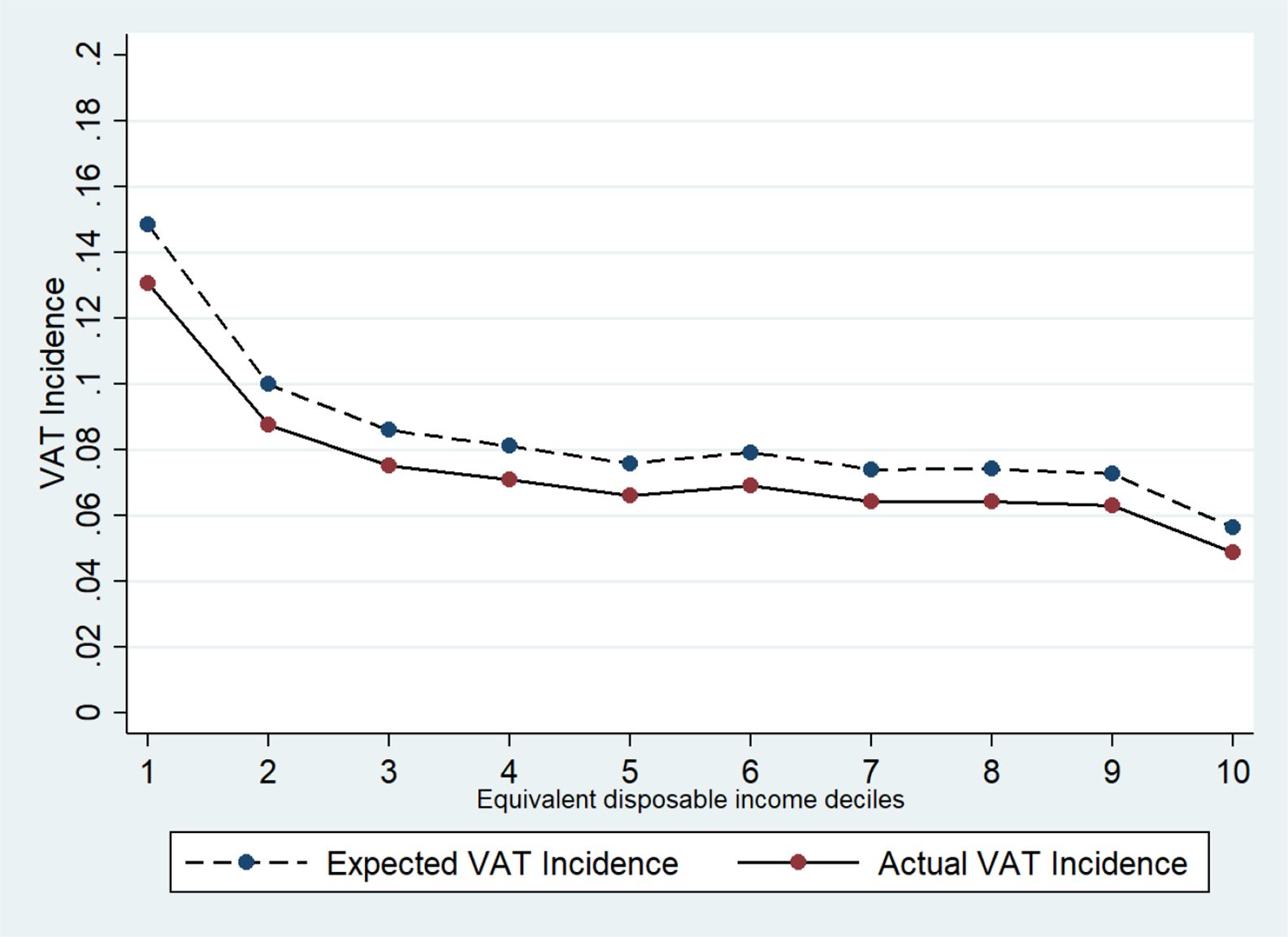
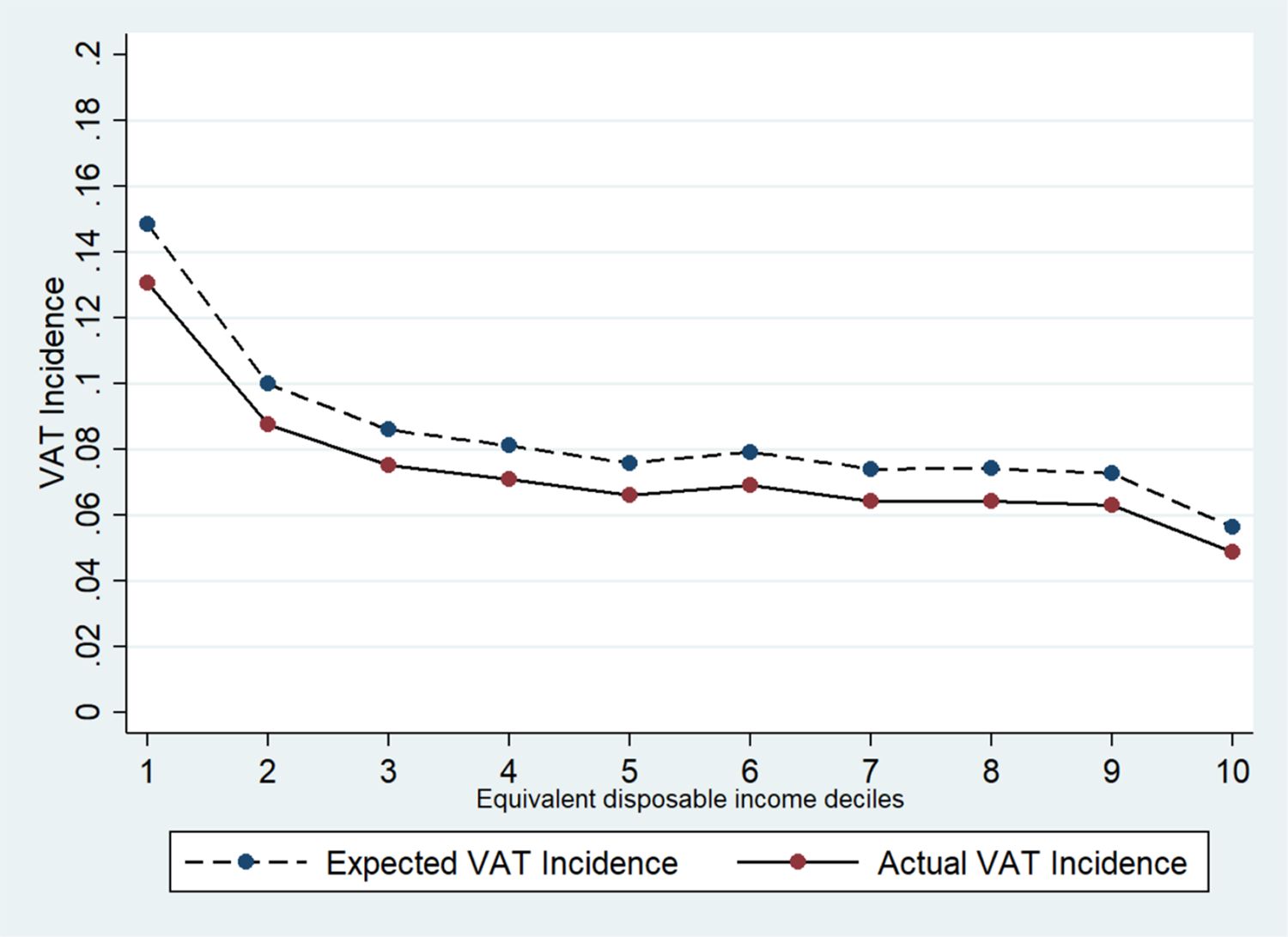
Figure 4 shows the actual and expected VAT incidence on households disposable income by equivalent disposable income deciles. 19 As expected, VAT is a regressive tax because low-income households spend a higher share of their income for consumption (and consequently for VAT) with respect to high-income households. Indeed, we find that in 2019, at aggregate level, households in the lowest income decile devote 13.4% of their income to VAT expenditure. Conversely, the highest income households spend only 4.7% of their income to pay VAT on goods (for more details see Appendix 3, Table A3).

VAT Incidence on Households Disposable Income, by Income Deciles. Source: Authors elaboration.
Our results on VAT incidence are not very different from recent findings by Centro Studi Confindustria (2019) but we found a slightly higher level of regressivity. 20 While we found a similar VAT incidence of 13% for the for the lowest income decile, for all the other deciles, Centro Studi Confindustria show a higher VAT incidence (between 10% and 9%) with respect to our findings (between 9% and 6%). For the highest income decile, this figure is even more pronounced because we found a VAT incidence of 4.7% while they find a VAT incidence of around 9%. The regressivity of VAT was confirmed also using different methodologies. For instance, Benassi and Randon (2020) rely on the stochastic dominance relationship between the income share distribution and the VAT burden distribution and provide evidence of VAT regressivity. Finally, our results show that the VAT incidence trend in Italy is similar to the one calculated on the average of other 26 OECD countries (see Thomas, 2020). 21
In order to have a complete picture of the households that bear the highest burden of VAT, we disaggregate data on VAT incidence by VAT rates (Figure 5). For goods with super reduced and reduced VAT rates (namely, 4%, 5%, and 10%), the incidence curve is flatter with respect to the one related to goods with a standard VAT rate (22%). However, the absolute difference in incidence between the highest and the lowest income deciles are 0.3, 1.9, and 6.3 percentage points, for super-reduced, reduced and standard VAT rates, respectively. This result shows that VAT is regressive, although by different degrees, for all VAT rates.
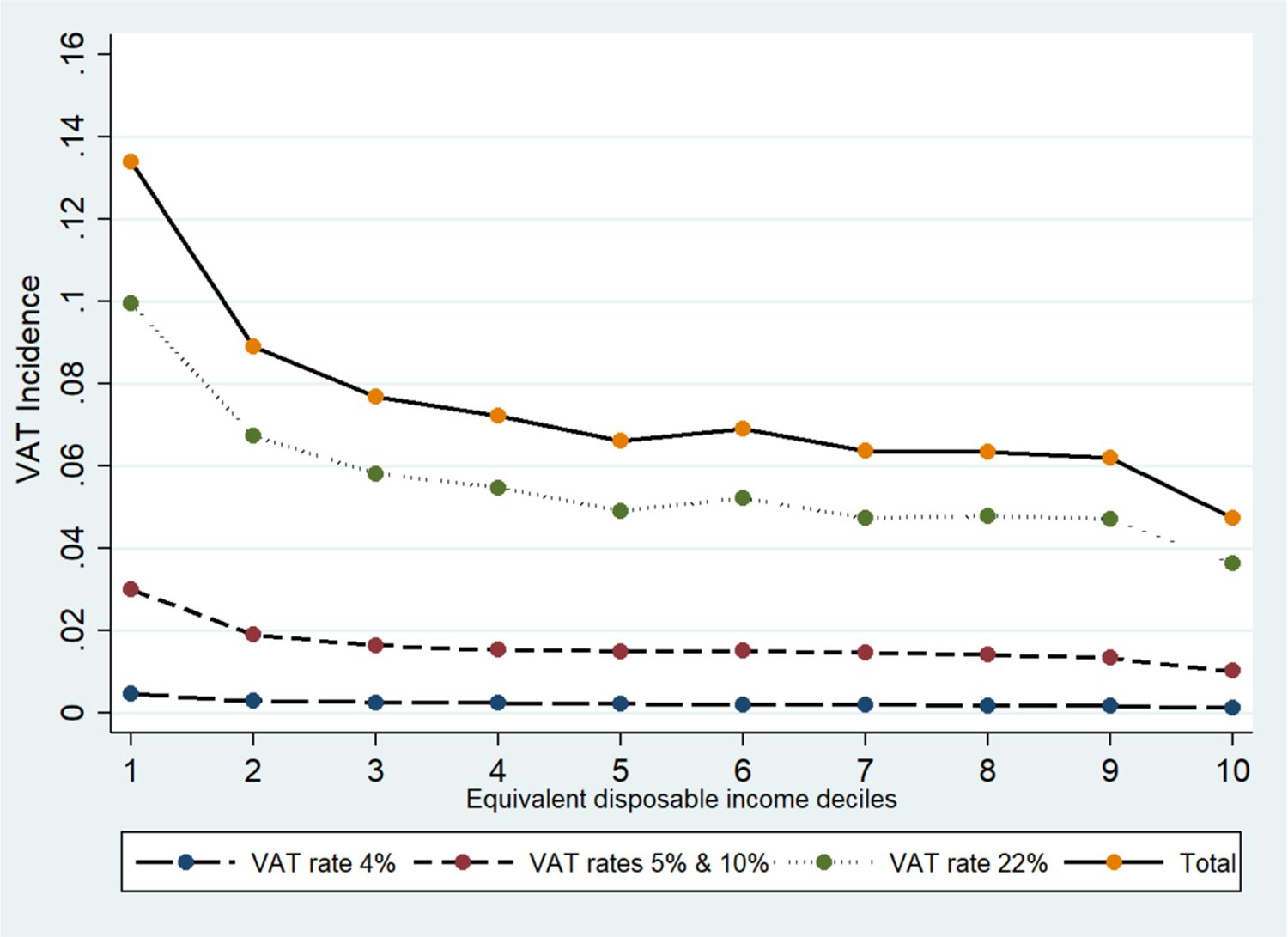
Actual VAT Incidence on Households Income, by Income Deciles and VAT Rates. Source: Authors elaboration.
More interestingly, the VAT incidence and the VAT gap vary by bundles of goods. Indeed, the VAT incidence curve is steeper for goods related to food and non-alcoholic beverages, transport, clothing and footwear, showing a stronger regressivity and a high burden for low-income households (see Appendix 4, Figure A4)22. Transport, food, and non-alcoholic beverages are (jointly with housing, water, gas, electricity, and other fuels) also the goods that absorb the highest share of households income. Moreover, not surprisingly, the share of income devoted to these goods is much higher for low-income households in comparison with the highest income ones (see Appendix 5,Figure A5).
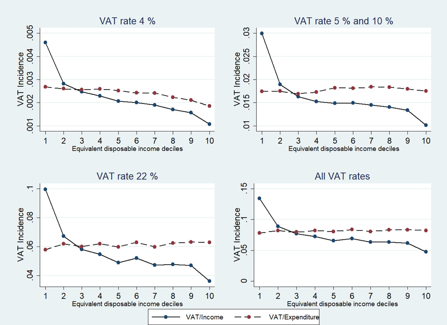
The results showed so far are based on the choice to measure the VAT incidence on current income. However, the high incidence of VAT on the lowest income deciles, can be due to two factors. The first one is usually related to under-reporting or misreporting errors in income data for the lowest deciles. To address this problem, we adjusted income by imputing unplausible low-income values to positive values (Section 4.1). The second one, is related to the use of current income instead of permanent income. Indeed, according to Gastaldi et al. (2016), in single-period analysis, findings about the regressivity of VAT may be upward biased by the presence, in the sample, of consumption smoothers, whose expenditure choices may not be affected by negative fluctuations in current income. The best option to check for this hypothesis would be to measure VAT incidence on lifetime income (Levell et al., 2020), but this data availability is extremely limited. To overcome these issues, several scholars suggest relying on expenditure as reference value for VAT incidence (for instance, Adam et al., 2011). Indeed, in some cases, and under the hypothesis of consumption smoothing, expenditure is used as a proxy for lifetime income. To account for this, we also estimate the VAT incidence on expenditure, and we found that, overall, the incidence curve is flat (Appendix 6,Figure A6). However, using expenditure as a reference to calculate VAT incidence has its drawbacks. First, as argued by Mirrlees et al. (2011), since low-income households may face borrowing constraints to smooth consumption, the most important indicator for them is still current income. Second, while measuring VAT incidence on current income may lead to an overestimation of VAT regressivity, the use of expenditure, as reference value, may lead to an underestimation of VAT regressivity. Underestimating regressivity is much risky, as it could favour policies which can produce long-term detrimental effects on low-income households at risk of poverty.
5. Simulation
In this section, we show an application of VATSIM-DF (II). It is worth noting that the proposed application is an exercise to show how a reform of the VAT system may affect the VAT burden on households. The proposed reform is an exercise to test the simulation model. Indeed, to design a reform of the VAT system one should consider the entire fiscal systems and account for the individuals behavioral responses to changes in VAT rates. 23
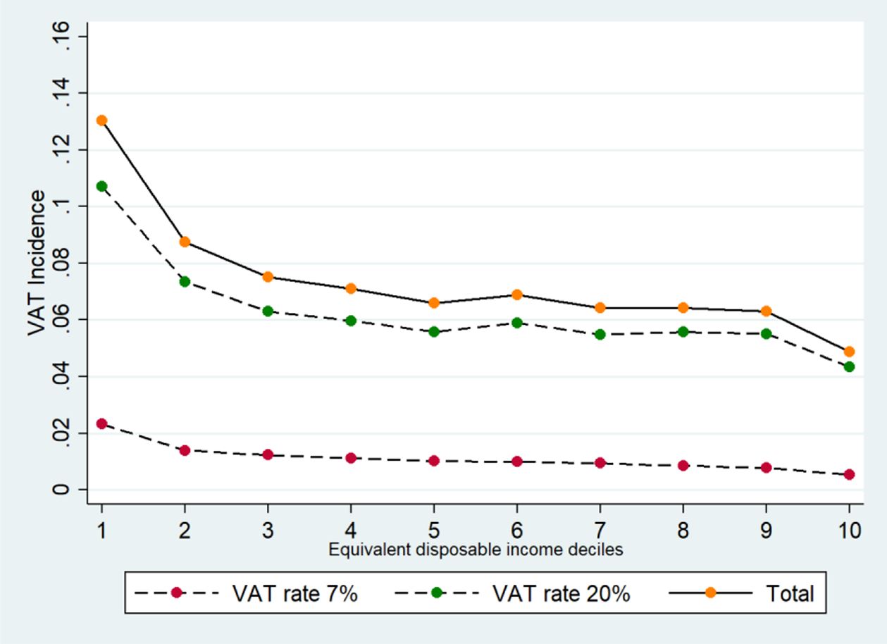
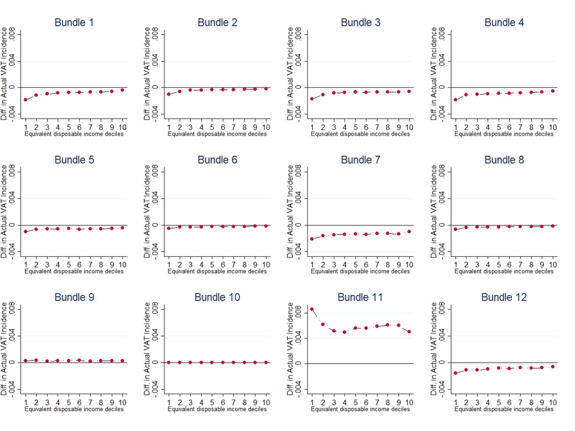
We analyse a scenario with a revenue neutral reform which sets two VAT rates of 7% and 20%. 24 In particular, the reduced VAT rate of 7% is applied to food and non-alcoholic beverage and to other goods and services currently subject to a VAT rate of 4%, 5%, and 10%. Also, we applied the VAT rate of 7% to some articles and products for personal care (such as, female sanitary towels and babies’ nappies). In our simulation, we assign a VAT rate of 20% to goods and services which are currently subject to the standard VAT rate of 22%. Appendix 7 (Table A7) provides details about the changes we applied to existing VAT rates. The primary role of VAT is not to stimulate or discourage the consumption of certain types of goods, which is the goal of other types of fiscal measures. 25 However, in our simulation we take into account social, cultural and environmental considerations made in the past by policy makers. Figure 6 shows the results of our simulation in terms of VAT incidence in aggregate terms (see Appendix 8,Figure A8, for further details). The simulation results show that the changes applied to VAT rates do not strongly affect the VAT burden on households, which is very similar to the one observed at current legislation. Indeed, in Figure 7, we report the difference in incidence between simulation and current legislation. Although the VAT burden on households is not subject to strong changes, we can observe that there is a slight reduction in incidence for low-income households and an even smaller increase in incidence for high income households. Most importantly, in Appendix 8 (Figure B8), we show that the VAT incidence, for food and non-alcoholic beverages, decreases for all households but it benefits most low-income households. The same applies to other sectors, such as clothing and footwear and housing, water, gas, electricity and other fuels. Conversely, the VAT burden on households visibly increases for restaurants and hotels, especially for low-income households.
VAT Incidence on Households Income at simulation rates. Source: Authors elaboration. Note: VAT simulation rates are 7% and 20%.
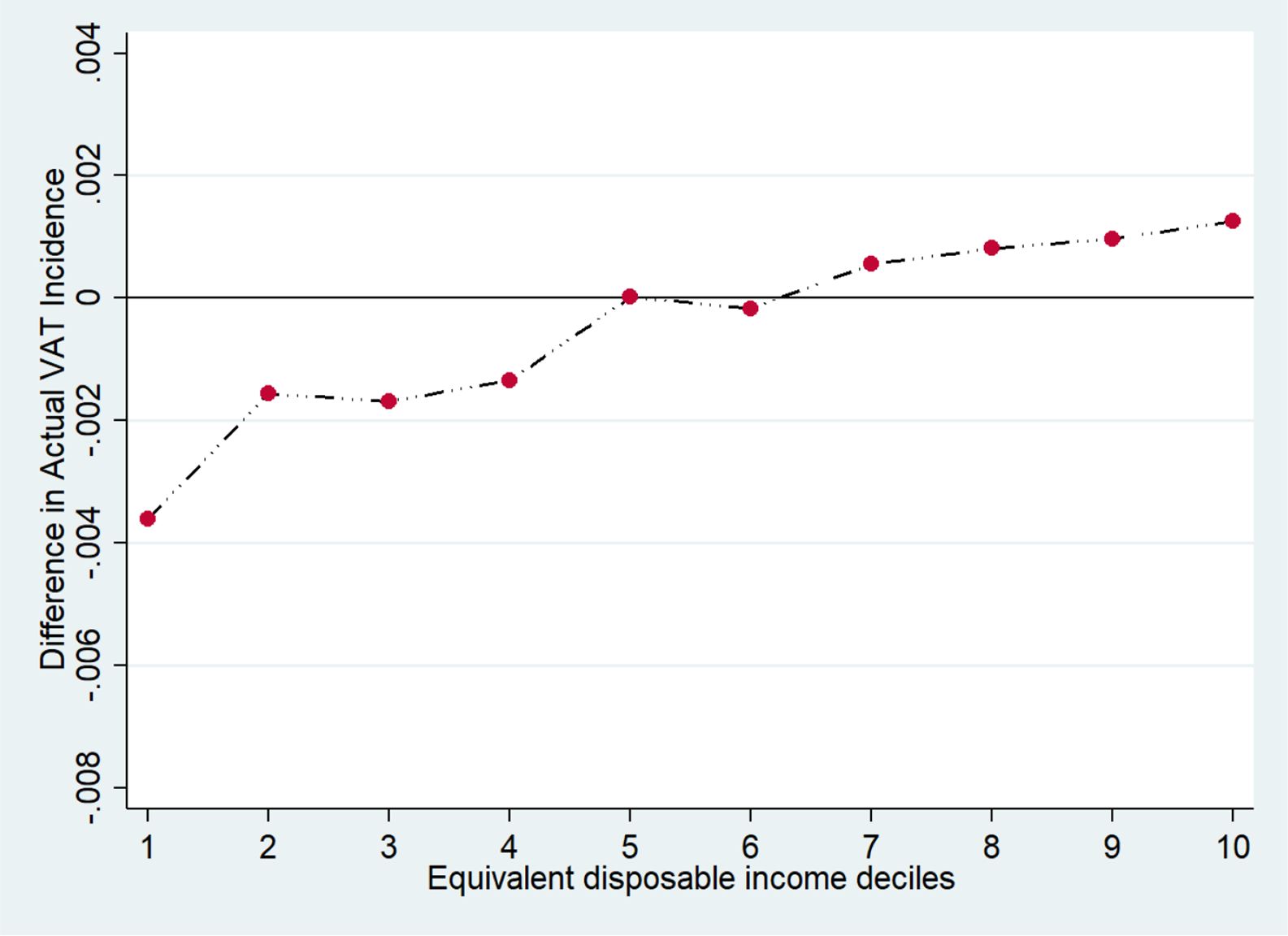

VAT Incidence difference between current legislation and simulation rates. Source: Authors elaboration.
6. Conclusion
The objective of this paper was to describe the VATSIM-DF (II), a new microsimulation model whose goals are to: (i) to estimate actual and expected VAT amounts; (ii) to assess the VAT incidence on household disposable income; (iii) and to simulate the effects of changes in fiscal policies. The main innovation of our model, with respect to the existing literature, is the creation and the use of a new dataset developed by implementing an original matching procedure based on tax register data, which outperforms other matching procedures commonly used in previous studies.
The model relies on two surveys about income and consumption which are merged one at a time with Tax Register data, through an exact matching based on tax codes. Then the two surveys are merged, between them, by a statistical matching relying on Tax Register data on income and on socio-demographic households characteristics. The resulting dataset (VATIC 2019) is a unique source of detailed data on income and expenditure, at the household level. Then survey data are adjusted to National Accounts data to obtain the most updated variables coherent with macroeconomic data. Finally, we provide the main microsimulation outputs. Indeed, thanks to this model, we can assess the actual and expected VAT revenue and the VAT gap. Most importantly, we estimate the level of regressivity of VAT in Italy, which is a crucial information to design policies able to account for the trade-off between equity and efficiency.
The motivation for this model was twofold. From the one side, we wanted to produce a reliable microsimulation tool which can support Italian policy makers to design VAT related policies. From the other, we aimed at contributing to the existing literature by providing a microsimulation model with original features. Indeed, the value added of VATSIM-DF (II), with respect to the existing models, are: (i) the creation of a unique dataset with data on income and consumption with a very high level of reliability, since the matching procedure relies on tax codes and Tax Register data; (ii) the adjustment of survey data on income and consumption to National Accounts data at the year of the simulation, which makes our estimations on VAT extremely coherent with the most updated macroeconomic data. To the best of our knowledge, there are not existing models in Italy with these features and this makes VATSIM-DF (II) a promising tool for reliable microsimulations about the distributional effects of VAT. We show that the procedure we used to create the dataset VATIC 2019, outperforms other methods used in the literature about microsimulation models in Italy. Also, we show an application of our model by testing a revenue neutral reform with two VAT rates. The reform consists only of two rates: a reduced VAT rate of 7% and an ordinary VAT rate of 20%. In addition to other basic goods, the reduced VAT rate is also applied to female sanitary towels and babies nappies. We show that this reform does not strongly affect the VAT burden on households. Conversely, it benefits low-income households reducing the VAT burden for basic goods and services (e.g. food and non-alcoholic beverages; clothing and footwear; and housing, water, gas, electricity and other fuels). However, the VAT burden on households visibly increases for restaurants and hotels, in particular for low-income households. A further extension of the VATSIM-DF (II) model, which will be described in a forthcoming paper, focuses on the behavioural effects produced by tax-shifts and changes in fiscal policies.
Footnotes
1.
Financed by the European Commission.
2.
3.
Details are provided in section 3.
4.
In other countries the HBS dataset include data on income.
5.
The matching procedure will be explained in detail in Section 3.
6.
Data analysis was conducted in STATA 14.
7.
Data about the individual tax codes are extremely confidential and are anonymized by SOGEI s.p.a.
8.
Another practical reason is that, in order to develop analyses on tax-shift from labour to consumption taxation, we integrate the VATSIM-DF (II) model with other models (e.g. TAXBEN-DF) which are based on SILC households.
9.
Estimations were conducted using the STATA package developed by Leuven and Sianesi (2003)
10.
4,239 HBS households are matched to one SILC household only, while the rest of the selected HBS observations are paired to more than one SILC household. This is due also to the fact that the SILC sample size is bigger than the HBS sample size.
11.
The methodology used to estimate weights for each VAT rate is the same used for the calculation of VAT for the European budget own resources, in the unpublished document received from the Ministry of Economy and Finance “Base di calcolo risorse proprie I.V.A. 2019”.
12.
HBS consumption data are usually underestimated. We can attribute the difference between the survey data and the National Accounts data to: (i) unintentional under-reporting due to recalling errors; (ii) intentional under-reporting motivated by tax evasion. Our methodology to adjust survey data to National Accounts data consists in a proportional assignment of expenditure values, for each asset. Indeed, while we adjust survey data to National Accounts, we do not consider differences across households, but we assume that the under-declaration is uniform among them. This assumption is consistent with the other steps of the model, in which tax evasion rates (applied to obtain actual VAT) varies across different goods or services, but do not depend on the households characteristics. A further development of our model will introduce evasion rates, which vary depending on households characteristics and seller types.
13.
As mentioned, in our model, we consider only evasion rates which vary across good, but which do not change across households depending on their characteristics.
14.
Istat estimates the evasion rates on economic sectors (NACE). We convert evasion rates on NACE to evasion rates first on CPA (by relying on a supply matrix) and then on COICOP (by relying on a transition matrix) (for more details, see the methodology implemented by Calà et al., 2020)
15.
We assume that the evasion for omitted invoicing is associated with B2C transactions, while the evasion for omitted declaration is entirely due to the B2B transaction.
16.
Disposable income is adjusted for in-kind social benefits.
17.
Also, in this case we make a proportional adjustment to all families, not considering their own characteristics and assuming that households have the same propensity to evade. A further development of this model will accounts for this aspect.
18.
We compared the households’ propensity to consume computed in the original survey data with the one calculated on the final dataset (adjusted to National Accounts), and we checked that the original propensity to consume was preserved.
19.
The incidence is computed as the total VAT paid by the each decile of households over each decile total disposable equivalent income. Also, we can compute the VAT incidence as follows: for each household, we calculate the rate between paid VAT and disposable equivalent income. Then, within each decile, we compute the mean and the corresponding confidence intervals (see Appendix 2, Figure A2).
20.
For this estimation, Centro Studi Confindustria (2019) relies on the EUROMOD-ITT v1.0 model with IT-SILC and HBS data.
21.
With respect to our study, Pacifico found a higher level of regressivity: see https://www.lavoce.info/archives/10062/ecco-chi-soffre-di-piu-con-laumento-delliva/
22.
For more details about the households consumption composition by bundle and income decile, see Figure B4
23.
These aspects are beyond the scope of this paper and are the focus of VATSIM-DF (III), a behavioural model that will be the focus of further research.
24.
The proposed reform is almost neutral because we allow a slight increase in the VAT revenue.
25.
Reduced VAT rates are often used to pursuing distributional effects and, actually, are proven to be effective in promoting progressivity (OECD and KIPF, 2014). However, they are less effective than other targeted measures in supporting poor households. Also, reduced rates aimed at pursuing social non-distributional objectives (i.e. stimulating consumption of books, restaurant foods, etc.) often provide equal or more benefits to the rich than to the poor (ibid.). This evidence leads to advocating also for different types of measures, rather than a mere change to the VAT system, to reach specific goals.
Appendix 1
Below, we show the results after a matching procedure based on estimated consumption relying on the SHIW data (see Table A1). Since we have access to the Tax register data, we show that a matching based on estimated consumption may pair households that are significantly different, on average, in Tax Register income (see Table B1). Finally, we show the consumption distribution before and after the matching based on SHIW as bridge dataset (see Figure A1). Comparing Figure 2 (Section 3.2) and Figure A1, we find that our matching procedure, based on Tax Register data, is more able to preserve the original consumption distribution with respect to a matching procedure based on estimated consumption.
Comparison between SILC and HBS Samples after a Matching based on SHIW
| Mean in SILC | Mean in HBS | p-value for difference | |
|---|---|---|---|
| Total consumption | 19,738.43 | 19,589.20 | 0.437 |
| First-earner age | 59.49 | 59.14 | 0.149 |
| First-earner sex | 0.59 | 0.63 | 0.000 |
| Household size | 2.16 | 2.12 | 0.011 |
| Number of children | 0.26 | 0.27 | 0.498 |
| First-earner occupation | |||
| Employed | 0.52 | 0.52 | 0.285 |
| Unemployed | 0.03 | 0.03 | 0.871 |
| Homemaker | 0.04 | 0.04 | 0.263 |
| Retired | 0.38 | 0.38 | 0.914 |
| Student, unable to work or other | 0.03 | 0.03 | 0.026 |
| First-earner education level | |||
| None | 0.04 | 0.03 | 0.098 |
| Primary education | 0.17 | 0.17 | 0.695 |
| Lower secondary education | 0.27 | 0.29 | 0.024 |
| Vocational education (2-3 years) | 0.07 | 0.07 | 0.243 |
| Upper secondary education | 0.29 | 0.30 | 0.350 |
| University bachelor’s degree | 0.13 | 0.12 | 0.237 |
| Post graduate education | 0.03 | 0.02 | 0.037 |
| Type of Family | |||
| Single | 0.37 | 0.43 | 0.000 |
| Couple with no children | 0.21 | 0.23 | 0.057 |
| Couple with 1 child | 0.16 | 0.16 | 1.000 |
| Couple with 2 or more children | 0.25 | 0.18 | 0.000 |
| Other | 0.00 | 0.00 | 0.000 |
Comparison between SILC and HBS samples after an alternative matching procedure based on estimated consumption relying on the SHIW dataset
| Tax Register variables not used in this matching procedure | Mean in SILC | Mean in HBS | p-value for difference |
|---|---|---|---|
| Tax Register household total income | 31,474.26 | 30,324.65 | 0.013 |
| Tax Register household taxable income | 30,584.36 | 29,429.39 | 0.008 |
| Tax Register first-earner total income | 1,641.48 | 1,397.99 | 0.001 |
| Tax Register first-earner taxable income | 3,260.84 | 3,057.20 | 0.424 |
| Tax Register household land and buildings income | 23,972.73 | 24,133.68 | 0.666 |
| Tax Register other household income | 23,158.80 | 23,220.48 | 0.863 |
-
Note: We computed total consumption in SILC by relying on SHIW estimates.

HBS Households Expenditures Distribution before and after a Matching based on estimated consumption using SHIW. Source: Authors elaboration.
Appendix 2
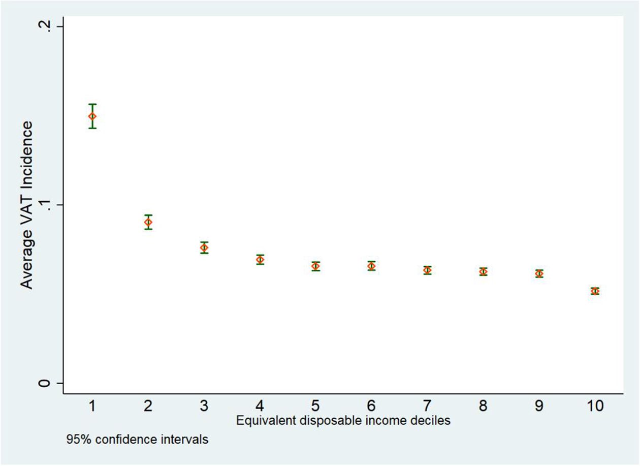

Actual VAT Incidence on Households Disposable Income, by Income Deciles. Source: Authors elaboration. Note: The graph shows the average VAT incidence within each households income decile and the corresponding confidence intervals.
Appendix 3
Expected and Actual VAT Incidence, by Equivalent Disposable Income Deciles
| Equivalent disposable income deciles | Total Disposable Income | Expected VAT | Actual VAT | Expected VAT Incidence on Income (%) | Actual VAT Incidence on Income (%) |
|---|---|---|---|---|---|
| 1 | 42,656,515,904 | 6,440,205,569 | 5,717,503,164 | 15.1 | 13.4 |
| 2 | 79,589,374,269 | 8,006,812,939 | 7,084,726,118 | 10.1 | 8.9 |
| 3 | 93,403,298,062 | 8,124,126,841 | 7,179,631,781 | 8.7 | 7.7 |
| 4 | 106,856,669,734 | 8,744,791,259 | 7,721,938,519 | 8.2 | 7.2 |
| 5 | 122,544,889,789 | 9,182,400,875 | 8,084,834,747 | 7.5 | 6.6 |
| 6 | 132,819,790,461 | 10,418,560,067 | 9,178,307,726 | 7.8 | 6.9 |
| 7 | 148,735,451,716 | 10,772,263,843 | 9,473,851,362 | 7.2 | 6.4 |
| 8 | 163,114,644,148 | 11,774,392,072 | 10,352,181,184 | 7.2 | 6.3 |
| 9 | 189,448,962,698 | 13,370,000,513 | 11,739,157,681 | 7.1 | 6.2 |
| 10 | 305,787,404,365 | 16,522,434,255 | 14,494,746,061 | 5.4 | 4.7 |
-
Source: Authors elaboration.
Appendix 4
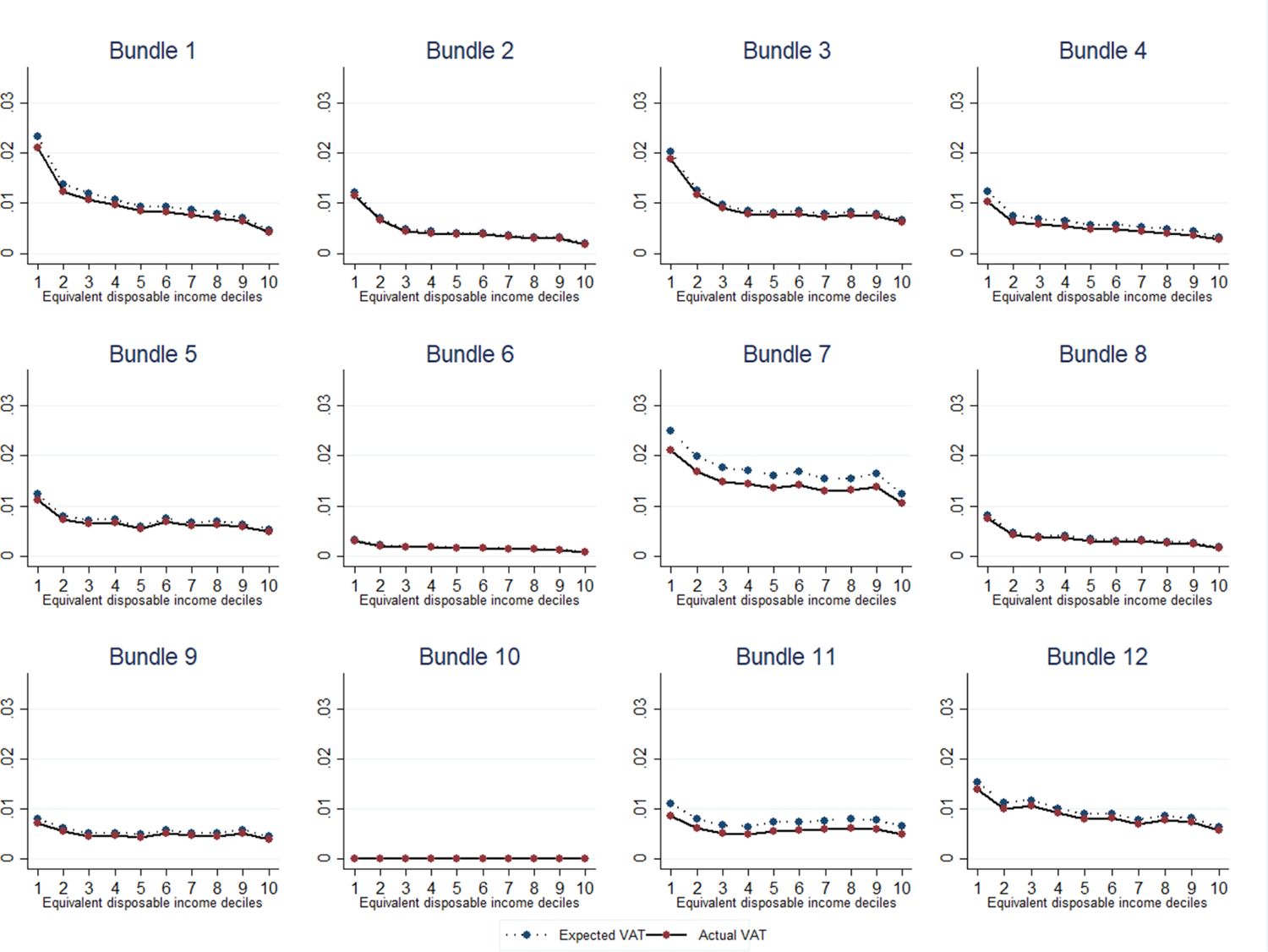
Actual and Expected VAT Incidence, by Bundle. Source: Authors elaboration. Note: The bundles refer, respectively, to: 1-Food and Non-Alcoholic Beverages; 2-Alcoholic Beverages and Tobacco; 3-Clothing and Footwear; 4-Housing, Water, Gas, Electricity and Other Fuels; 5-Furnishings, Household Equipment and Routine Maintenance Of The House; 6-Health; 7-Transport; 8-Communications; 9-Recreation and Culture; 10-Education; 11-Restaurants and Hotels; 12-Miscellaneous Goods and Services.

=Consumption Composition, by Bundle and Income Deciles. Source: Authors elaboration. Note: The bundles refer, respectively, to: 1-Food and Non-Alcoholic Beverages; 2-Alcoholic Beverages and Tobacco; 3-Clothing and Footwear; 4-Housing, Water, Gas, Electricity and Other Fuels; 5-Furnishings, Household Equipment and Routine Maintenance Of The House; 6-Health; 7-Transport; 8-Communications; 9-Recreation and Culture; 10-Education; 11-Restaurants and Hotels; 12-Miscellaneous Goods and Services.
Appendix 5
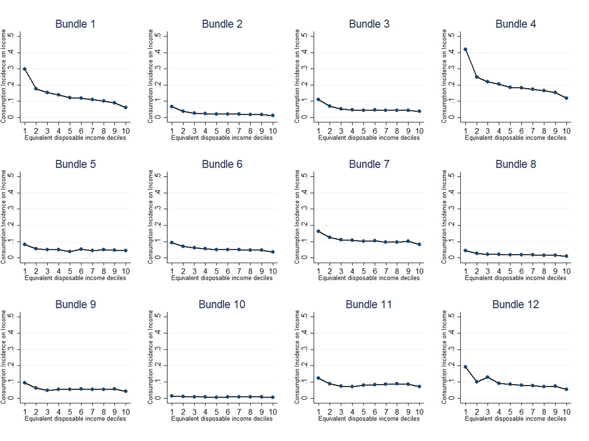
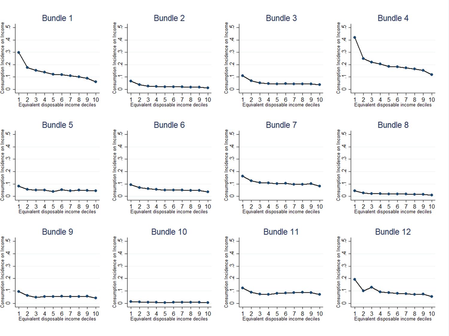
Consumption Incidence on Income, by Bundle. Source: Authors elaboration. Note: The bundles refer, respectively, to: 1-Food and Non-Alcoholic Beverages; 2-Alcoholic Beverages and Tobacco; 3-Clothing and Footwear; 4-Housing, Water, Gas, Electricity and Other Fuels; 5-Furnishings, Household Equipment and Routine Maintenance Of The House; 6-Health; 7-Transport; 8-Communications; 9-Recreation and Culture; 10-Education; 11-Restaurants and Hotels; 12-Miscellaneous Goods and Services.
Appendix 6

VAT Incidence on Income and Expenditure, by VAT Rates and Income Deciles. Source: Authors elaboration.
Appendix 7
VAT Simulation Rates
| Bundles | Group of expenditures | VAT rates in current legislation | VAT simulation rates |
|---|---|---|---|
| Food and non-Alcoholic Beverages | Rice, pasta products and couscous | 4%, 10% | 7% |
| Food and non-Alcoholic Beverages | Bread, flours and other cereals | 4% | 7% |
| Food and non-Alcoholic Beverages | Pizza and quiche, other bakery products, breakfast cereals, other cereal products | 10% | 7% |
| Food and non-Alcoholic Beverages | Meat and meat preparations | 10% | 7% |
| Food and non-Alcoholic Beverages | Fresh, chilled or frozen fish. Other preserved or processed fish and seafood-based preparations | 10% | 7% |
| Food and non-Alcoholic Beverages | Fresh, chilled or frozen seafood | 10%, 22% | 7% |
| Food and non-Alcoholic Beverages | Milk and cheese | 4% | 7% |
| Food and non-Alcoholic Beverages | Preserved milk, yoghurt, other milk products | 10% | 7% |
| Food and non-Alcoholic Beverages | Eggs | 10% | 7% |
| Food and non-Alcoholic Beverages | Butter, olive oil, other edible oils | 4% | 7% |
| Food and non-Alcoholic Beverages | Other edible animal fats | 10% | 7% |
| Food and non-Alcoholic Beverages | Fresh, chilled or frozen fruit | 4% | 7% |
| Food and non-Alcoholic Beverages | Dried fruit and nuts | 4%, 10% | 7% |
| Food and non-Alcoholic Beverages | Preserved fruit and fruit-based products | 10%, 22% | 7% |
| Food and non-Alcoholic Beverages | Fresh, chilled or dried vegetables, other preserved or processed vegetables, crisps | 4%, 10% | 7% |
| Food and non-Alcoholic Beverages | Frozen vegetables, potatoes and other tubers and products of tuber vegetables | 4% | 7% |
| Food and non-Alcoholic Beverages | Sugar, jams, marmalades, honey, chocolate, confectionery products, edible ices and ice cream | 10% | 7% |
| Food and non-Alcoholic Beverages | Artificial sugar substitutes | 22% | 20% |
| Food and non-Alcoholic Beverages | Sauces, condiments, baby food, ready-made meals, other food products n.e.c. | 10% | 7% |
| Food and non-Alcoholic Beverages | Salt, spices and culinary herbs | 5%, 10%, 22% | 7% |
| Food and non-Alcoholic Beverages | Coffee and tea | 10%, 22% | 7% |
| Food and non-Alcoholic Beverages | Cocoa and powdered chocolate | 10% | 7% |
| Food and non-Alcoholic Beverages | Mineral waters, soft drinks, fruit and vegetable juices | 22% | 20% |
| Alcoholic Beverages and Tobacco | Spirits and liqueurs | 22% | 20% |
| Alcoholic Beverages and Tobacco | Tobacco | 22% | 20% |
| Clothing and Footwear | Clothing and footwear | 22% | 20% |
| Housing, Water, Gas, Electricity and Other Fuels | Actual rentals paid by tenants for primary and secondary residences | 0%, 10% | 0%, 20% |
| Housing, Water, Gas, Electricity and Other Fuels | Garage rentals and other rentals paid by tenants | 0%, 22% | 0%, 20% |
| Housing, Water, Gas, Electricity and Other Fuels | Imputed rentals of owner-occupiers and other imputed rentals | 0% | 0% |
| Housing, Water, Gas, Electricity and Other Fuels | Materials for the maintenance and repair of the dwelling | 22% | 20% |
| Housing, Water, Gas, Electricity and Other Fuels | Services for the maintenance and repair of the dwelling | 10% | 7% |
| Housing, Water, Gas, Electricity and Other Fuels | Water supply | 10% | 7% |
| Housing, Water, Gas, Electricity and Other Fuels | Refuse and sewage collection | 0% | 0% |
| Housing, Water, Gas, Electricity and Other Fuels | Maintenance charges in multi-occupied buildings | 0%, 10%, 22% | 0%, 7%, 20% |
| Housing, Water, Gas, Electricity and Other Fuels | Security services | 22% | 20% |
| Housing, Water, Gas, Electricity and Other Fuels | Other services related to dwelling | 10%, 22% | 7%, 20% |
| Housing, Water, Gas, Electricity and Other Fuels | Electricity | 10% | 7% |
| Housing, Water, Gas, Electricity and Other Fuels | Natural gas through networks, liquefied hydrocarbons | 10%, 22% | 7%, 20% |
| Housing, Water, Gas, Electricity and Other Fuels | Liquid fuels, solid fuels | 22% | 20% |
| Housing, Water, Gas, Electricity and Other Fuels | Other energy for heating and cooling | 10% | 7% |
| Furnishings, Household Equipment and Routine Household Maintenance | Furniture, furnishings, carpets and floor coverings | 22% | 20% |
| Furnishings, Household Equipment and Routine Household Maintenance | Services of laying of fitted carpets and floor coverings | 10% | 7% |
| Furnishings, Household Equipment and Routine Household Maintenance | Household textiles | 22% | 20% |
| Furnishings, Household Equipment and Routine Household Maintenance | Major and small household appliances | 22% | 20% |
| Furnishings, Household Equipment and Routine Household Maintenance | Glassware, tableware and household utensils | 22% | 20% |
| Furnishings, Household Equipment and Routine Household Maintenance | Domestic services by paid staff | 0% | 0% |
| Furnishings, Household Equipment and Routine Household Maintenance | Other goods and services for routine household maintenance | 22% | 20% |
| Health | Pharmaceutical products | 10%, 22% | 7%, 20% |
| Health | Therapeutic appliances and equipment | 4% | 7% |
| Health | Repair of therapeutic appliances and equipment | 22% | 20% |
| Health | Out-patient and hospital services | 0% | 0% |
| Transport | New motor cars | 4%, 22% | 7%, 20% |
| Transport | Second-hand motor cars | 0%, 4%, 22% | 0%, 7%, 20% |
| Transport | Motor cycles and bicycles | 22% | 20% |
| Transport | Spare parts and accessories for personal transport equipment | 22% | 20% |
| Transport | Fuels and lubricants for personal transport equipment. Maintenance, repair and other services in respect of personal transport equipment | 22% | 20% |
| Transport | Driving lessons, tests, licences and road worthiness tests | 0%, 22% | 0%, 20% |
| Transport | Passenger transport by railway | 0%, 10% | 0%, 7% |
| Transport | Passenger transport by road | 0%, 10% | 0%, 7% |
| Transport | Passenger transport by air | 0%, 10% | 0%, 7% |
| Transport | Passenger transport by sea and inland waterway | 0%, 5%, 10% | 0%, 7% |
| Transport | Combined passenger transport | 0%, 5%, 10% | 0%, 7% |
| Transport | Funicular, cable-car and chair-lift transport | 10% | 7% |
| Transport | Other purchased transport services | 22% | 20% |
| Communication | Postal services | 0%, 22% | 0%, 20% |
| Communication | Telephone and telefax equipment | 22% | 20% |
| Communication | Telephone and telefax services and other information transmission services | 22% | 20% |
| Recreation and Culture | Equipment for the reception, recording and reproduction of sound and picture. Other major durables for recreation and culture | 22% | 20% |
| Recreation and Culture | Games, toys and hobbies. Equipment for sport, camping and open-air recreation | 22% | 20% |
| Recreation and Culture | Plants and flowers | 10% | 20% |
| Recreation and Culture | Garden products. Pets and related products and services | 22% | 20% |
| Recreation and Culture | Recreational and sporting services | 10%, 22% | 20% |
| Recreation and Culture | Cinemas, theatres, concerts | 10% | 20% |
| Recreation and Culture | Museums, libraries, zoological gardens | 0% | 0% |
| Recreation and Culture | Television and radio licence fees, subscriptions | 0%, 4%, 22% | 0%, 7%, 20% |
| Recreation and Culture | Hire of equipment and accessories for culture, photographic services, other cultural services | 22% | 20% |
| Recreation and Culture | Games of chance | 0% | 0% |
| Recreation and Culture | Books | 4% | 7% |
| Recreation and Culture | Binding services and E-book downloads | 22% | 20% |
| Recreation and Culture | Newspapers and periodicals | 4% | 7% |
| Recreation and Culture | Miscellaneous printed matter. Stationery and drawing materials | 22% | 20% |
| Recreation and Culture | Package domestic holidays | 10%, 22% | 20% |
| Recreation and Culture | Package international holidays | 0%, 22% | 0%, 20% |
| Education | Education | 0% | 0% |
| Restaurants and Hotels | Restaurants, cafés and the like | 10% | 20% |
| Restaurants and Hotels | Canteens | 4% | 7% |
| Restaurants and Hotels | Accommodation services | 10% | 20% |
| Miscellaneous Goods and Services | Hairdressing salons and personal grooming establishments. Appliances, articles and products for personal care. Personal effects n.e.c. | 22% | 20% |
| Miscellaneous Goods and Services | Female sanitary towels and babies nappies | 22% | 7% |
| Miscellaneous Goods and Services | Child care services | 0% | 0% |
| Miscellaneous Goods and Services | Retirement homes for elderly persons and residences for disabled persons. Services to maintain people in their private homes | 0%, 4%, 5%, 10%, 22% | 0%, 7%, 20% |
| Miscellaneous Goods and Services | Consuelling | 22% | 20% |
| Miscellaneous Goods and Services | Insurance | 0% | 0% |
| Miscellaneous Goods and Services | Other financial services n.e.c. | 0%, 22% | 0%, 20% |
-
Source: Authors elaboration.
Appendix 8

Actual VAT Incidence on Households Income at Simulation Rates, by VAT Rates. Source: Authors elaboration.
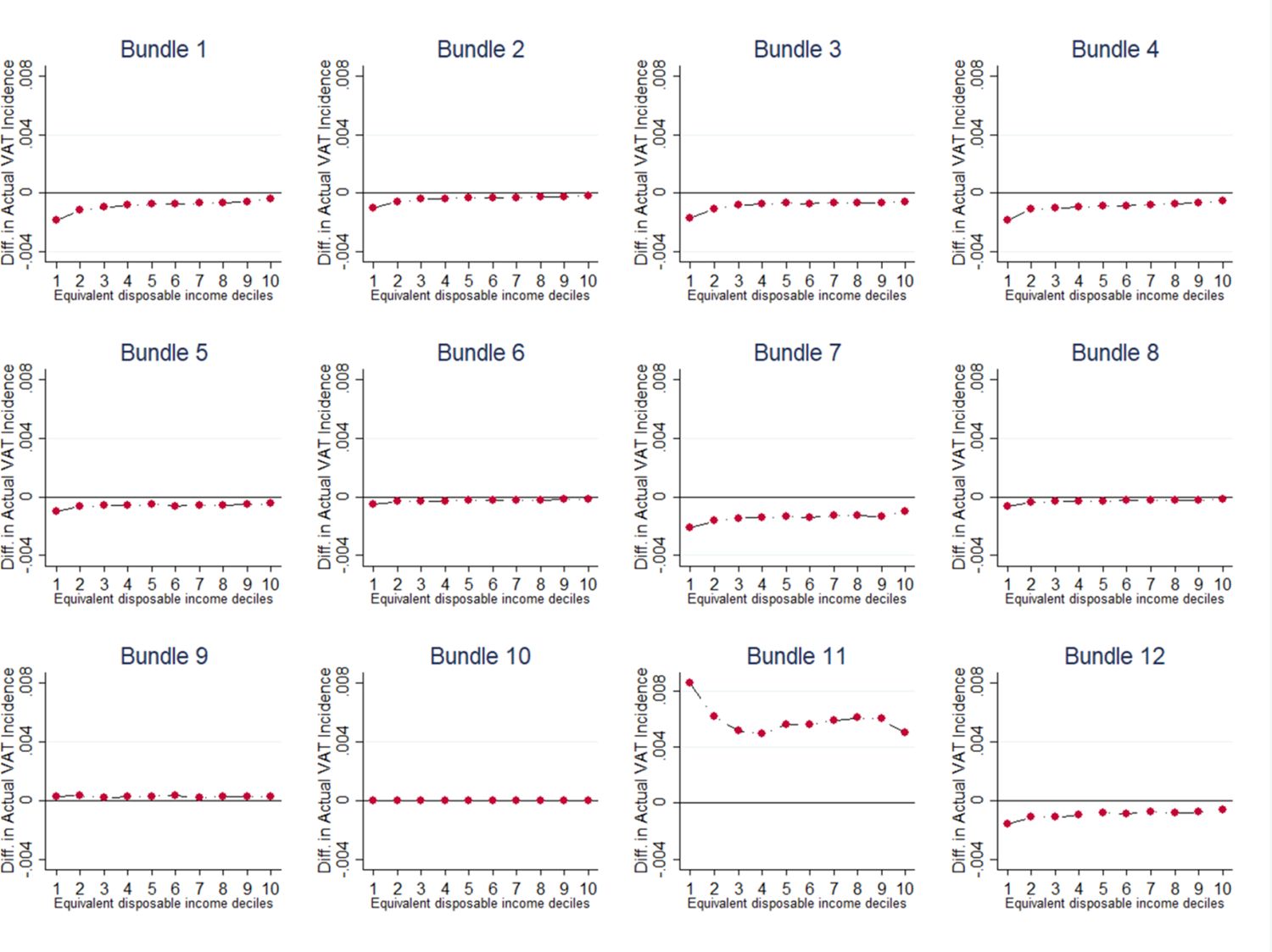
VAT Incidence Difference between Simulation and Current Legislation Rates, by Bundle. Source: Authors elaboration. Note: The bundles refer, respectively, to: 1-Food and Non-Alcoholic Beverages; 2-Alcoholic Beverages and Tobacco; 3-Clothing and Footwear; 4-Housing, Water, Gas, Electricity and Other Fuels; 5-Furnishings, Household Equipment and Routine Maintenance Of The House; 6-Health; 7-Transport; 8-Communications; 9-Recreation and Culture; 10-Education; 11-Restaurants and Hotels; 12-Miscellaneous Goods and Services.
References
-
1
TAXUD/2010/DE/328, FWC No.TAXUD/2010/CC/104, Institute for Fiscal Studies (Project Leader)A retrospective evaluation of elements of the EU VAT system: Final report, TAXUD/2010/DE/328, FWC No.TAXUD/2010/CC/104, Institute for Fiscal Studies (Project Leader).
-
2
Fiscal Reforms during Fiscal Consolidation: The Case of ItalyFinanz-Archiv: Zeitschrift Fur Das Gesamte Finanzwesen 68 :445–465.https://doi.org/10.1628/001522112X659574
-
3
Dipartimento Di Economia Politica, Università Di ModenaMAPP98: un modello di analisi delle politiche pubbliche, in «Materiali di discussione», n. 331, Dipartimento Di Economia Politica, Università Di Modena.
-
4
The recent reforms of the Italian personal income tax: distributive and efficiency effectsRivista Italiana Degli Economisti 14 :191–218.
-
5
DEMB Working Paper Series, Dipartimento Di Economia Marco Biagi - Università Di Modena e Reggio EmiliaImputation of missing expenditure information in standard household income surveys, DEMB Working Paper Series, Dipartimento Di Economia Marco Biagi - Università Di Modena e Reggio Emilia.
-
6
The distribution of the tax burden and the income distribution: theory and empirical evidenceEconomia Politica 38 :1087–1108.https://doi.org/10.1007/s40888-020-00207-3
-
7
Faculty of Economics, University of CambridgeEur3: A prototype European tax-benefit model (no.9723), Faculty of Economics, University of Cambridge.
-
8
Ministry of Economy and Finance, Department of FinanceA Methodological Note on the Value Added Tax Simulation Model - DF (I), Ministry of Economy and Finance, Department of Finance.
-
9
Toward a Comprehensive Tax Reform for ItalyIMF Working Papers 20 :1.https://doi.org/10.5089/9781513529226.001
- 10
-
11
Euromod Country ReportsEuromod Country Report: Italy 2014-2017, Euromod Country Reports.
-
12
Bank of Italy Temi Di Discussione (Working Paper) No, 908Asking income and consumption questions in the same survey: what are the risks?, Bank of Italy Temi Di Discussione (Working Paper) No, 908.
-
13
Bank of Italy Occasional Paper, (394)BIMic: The Bank of Italy microsimulation model for the Italian tax and benefit system, Bank of Italy Occasional Paper, (394).
-
14
(No. 1244) Bank of Italy, Economic Research and International Relations Area.Shifting taxes from labor to consumption: the efficiency equity trade-off, (No. 1244) Bank of Italy, Economic Research and International Relations Area..
-
15
EUROMOD Technical Note EMTN 3.0EUROMOD Extension to Indirect Taxation: Final Report, EUROMOD Technical Note EMTN 3.0, Colchester, Institute for Social and Economic Research, University of Essex.
-
16
EdiesseLa partita doppia del welfare: una base informativa originale per dibattere di tassazione e riforma dell’intervento pubblico: XIV rapporto CER-SPI, Ediesse.
-
17
Statistical matching of income and consumption expendituresInternational Journal of Economic Sciences 3 :50–65.
-
18
Working Paper SIEP 09Progressivity-Improving VAT Reforms in Italy, Working Paper SIEP 09.
-
19
Regressivity-Reducing VAT ReformsInternational Journal of Microsimulation 10 :39–72.https://doi.org/10.34196/ijm.00149
-
20
A Tax-Benefit Microsimulation Model for Italy: A Partial Evaluation of Fiscal Consolidation in the Period 2011-2014SSRN Electronic Journal 1.https://doi.org/10.2139/ssrn.2665547
-
21
Microsimulation Unit, Department of Applied Economics, University of CambridgeAn introduction to EUROMOD, Microsimulation Unit, Department of Applied Economics, University of Cambridge.
-
22
IstatIndagine sul reddito e le condizioni di vita delle famiglie (EU-SILC). Dati trasversali 2018 Dati longitudinali 2015-2018. Aspetti metodologici dell’indagine, Istat.
-
23
IstatIndagine sulle spese delle famiglie, Periodo di riferimento: anno 2017. Aspetti metodologici dell’indagine, Istat.
- 24
- 25
- 26
- 27
-
28
Statistical Software Components S432001, Boston College Department of Economics, Revised 01 Feb 2018PSMATCH2: Stata module to perform full Mahalanobis and propensity score matching, common support graphing, and covariate imbalance testing, Statistical Software Components S432001, Boston College Department of Economics, Revised 01 Feb 2018.
-
29
Mobility and the lifetime distributional impact of tax and transfer reformsInternational Tax and Public Finance 28 :751–793.https://doi.org/10.1007/s10797-020-09627-0
-
30
Studi e Approfondimenti IRPETIl modello di microsimulazione dell’Irpet MicroReg: aggiornamenti ed estensioni, Studi e Approfondimenti IRPET.
-
31
Pavia, Dipartimento Di Economia Pubblica e TerritorialeLa distribuzione del carico fiscale in Italia: un modello di microsimulazione, Pavia, Dipartimento Di Economia Pubblica e Territoriale.
-
32
Institute for Fiscal StudiesTax by Design: The Mirrlees Review, Institute for Fiscal Studies.
-
33
OECD Tax Policy Studies, No.22The Distributional Effects of Consumption Taxes in OECD Countries, OECD Tax Policy Studies, No.22, Paris, OECD Publishing, 10.1787/9789264224520-en.
-
34
Developing a static microsimulation model for the analysis of housing taxation in ItalyInternational Journal of Microsimulation 4 :73–85.https://doi.org/10.34196/ijm.00054
-
35
Working Papers 164, University of Rome La Sapienza, Department of Public EconomicsMicro data fusion of italian expenditures and incomes surveys, Working Papers 164, University of Rome La Sapienza, Department of Public Economics.
-
36
Data fusion: identification problems, validity, and multiple imputationAustrian Journal of Statistics 33 :153–171.
-
37
The central role of the propensity score in observational studies for causal effectsBiometrika 70 :41–55.https://doi.org/10.1093/biomet/70.1.41
-
38
Department of Public Policy and Public Choice-POLIS, Working Paper 63Propensity score matching: un’applicazione per la creazione di un database integrato ISTAT-Banca d’Italia, Department of Public Policy and Public Choice-POLIS, Working Paper 63.
-
39
University of Genova DEP Working Paper, 7L’ipotesi di tax-shift dal lavoro ai consumi in Italia: un’analisi di microsimulazione fiscale utilizzando il modello EUROMOD, University of Genova DEP Working Paper, 7.
-
40
OECD Taxation Working Papers, (49), 0_1-51Reassessing the regressivity of the VAT, OECD Taxation Working Papers, (49), 0_1-51.
Article and author information
Author details
Funding
No specific funding for this article is reported.
Acknowledgements
We are grateful to Silvia Carta, Luca Signorelli, Valerio Calà for the technical support and to Maria Teresa Monteduro, Giorgio Mongelli, Paolo Di Caro, and Silvia Giannini for helpful comments.
Publication history
- Version of Record published: December 31, 2021 (version 1)
Copyright
© 2021, Cirillo et al.
This article is distributed under the terms of the Creative Commons Attribution License, which permits unrestricted use and redistribution provided that the original author and source are credited.