Comparing Register and Survey Wealth Data
- National Institute of Economic Research, Sweden
- Department of Economics, Sweden
Abstract
Survey measures of wealth are error prone with a relatively large error variance. The errors are not uncorrelated with the true values but tend to have a negative correlation, which implies that wealthy people tend to underreport and less wealthy to over report. There is no general tendency of survey data to underestimate mean wealth with the exception of the last percentile. The underestimate of the wealth of the very rich is however not due to underreporting but rather to selective nonresponse. Using simple models this paper discusses consequences of error prone wealth data.
1. Introduction
Wealth surveys often include quite diverse data collection operations ranging from general purpose surveys with just a few wealth questions to surveys specialized on wealth. It is natural that coverage, definitions and quality varies between these studies. The more we understand about these differences the better our analysis become.
The difficulties in collecting wealth data in surveys are well-known. There are severe unit and item nonresponse problems – in particular in the two ends of the wealth distribution. There are difficulties for respondents to value their assets correctly and in a short interview it is not always possible to ask the respondent to get out relevant documentation which implies that they tend to “shoot from the hip”. There is also an issue of timing. Some surveys will get estimates as of the day of interview and because a survey is usually in the field several months up to a year, responses might apply to very different market situations. Other surveys ask for estimates as of a particular date, for instance the last day of a year, which might create memory problems or people might just give current estimates anyway.
Register data, depending on their origin, may have less of problems with response and measurement errors, but most of these data are collected primarily for administrative and not for statistical purposes. As a result, concepts and units are not always ideal for economic analysis and data on certain assets might not be collected at all. If wealth data come from self-assessments in the income taxation process, there are good reasons to believe that people have underreported assets and perhaps even overreported liabilities in order to reduce taxes. In the Swedish taxation procedure this source of error is substantially reduced and perhaps almost eliminated, because it is not the taxpayer who reports to the tax authorities about his assets and liabilities, but banks, insurance companies, brokers and housing associations. Every year in April the taxpayer obtains a statement from the tax office which lists all assets and liabilities reported to the authorities as of the last of December the previous year. If the taxpayer disagrees it is possible to appeal the numbers presented and if he can present a good case the tax office will adjust the numbers. If the taxpayer and the tax office disagree the taxpayer can appeal to court. Register data usually include corrections made by the tax offices but not the outcome of court procedures which may take long time.
For these reasons Swedish register data on financial assets and liabilities are generally considered so accurate that they can be used to validate survey data, and this is the topic of this paper. There are certainly remaining problems of comparison which will be discussed below, but first a few thoughts about the concept of a measurement error.
Even if there were no errors at all in register data it is not obvious that we want to define the measurement error in the survey by the difference between the survey and the register measures. One could argue that people take decisions based on the information they have even if it is incomplete and error prone. What we need for economic analysis is then the information people actually have, when they take their decisions, not the “true” register value. For instance, if a house owner thinks that the market value of the house is say 5 millions, he might take the decision to increase his mortgage, while if he had known that it only was 4 millions he might not have done so. However, if people act on erroneous information, they make mistakes and do not behave in an optimal way, and sooner or later they will discover their mistakes. They therefore have incentives to seek true information before they take decisions. A person who wants to sell shares certainly looks up the latest quote before he takes a decision about selling. The survey situation differs in this respect. The respondent has not the same incentive to seek the true response to questions about the market value of assets and the exact magnitude of liabilities as if he was to buy or sell assets.
At least when it comes to financial assets it is for these reasons meaningful to define the measurement error as the difference between the survey response and a “true” market value. But what do we mean by a “true” market value? The price of most financial assets is determined on well-functioning markets and we can rather easily get market quotes. There is though an issue of timing and volatility. Alternatively to the latest quote, one might like to use the average quote for the last day, week or month. In this study we will use the end of day quote for the last trading day in 2002 and 2003 respectively.
The market value of a house or any real property is not determined as easy, because a house is more or less unique depending on neighbourhood, size, design, equipment, etc. One can try to find out what similar houses in the same neighbourhood have sold for, but every house is valued by potential customers at the time the property is put on the market and it is not possible to know the market price until the property is sold. What people believe about the market value of their house and what they respond in a survey might therefore vary quite a lot depending on how closely they have followed the local housing market. In Sweden people are guided by the tax assessed value given to every house, which in principle should be about 75 percent of the market value. Statistics Sweden uses market quotes for recently sold houses and the tax assessed value to estimate the market value of single houses, but there is obviously an error margin also in these estimates, a problem we will return to.
In the sequel we will first give a descriptive analysis of our data, then in section 3 compare the right tail of survey and register estimates of the distribution of net worth using register data from 2002 and a survey from the same year as well as data from the first Swedish wave of the SHARE-survey with corresponding register data for 2003. In section 4 follows an analysis of measurement errors in the latter survey, and there is also a discussion of their potential consequences. The analysis in this section compares survey and register data for respondents, while any selective non-response is ignored. Johansson and Klevmarken (2008) analysed the properties of non-response in the RAND-UU survey, while there is not yet any corresponding study of the SHARE-SE sample. Johansson and Klevmarken (2008) found that non-response primarily arose among people with little wealth and small incomes.
2. Data sources
We use data from four sources: Register data from the 2002 and 2003 LINDA supplemented with assets and liabilities, sales data for real property, and survey data from the UU-RAND 2002 and the 2003 SHARE-SE surveys.
LINDA is a longitudinal sample of register data maintained by Statistics Sweden. It includes demographic and socio-economic variables with a focus on labour market status, incomes and taxes. The sample size is some 700,000 for each of the years 2002 and 2003. Both waves are proper random samples from the Swedish population.1
For tax purposes ownership of assets and liabilities is always individual, this implies that it is possible to add up gross and net wealth for a single individual. This does not exclude that more than one person can own, for instance a house. Each individual’s share is multiplied with the market value and registered to the individual. The same principles apply for liabilities.2 Even if it is technically possible to obtain a wealth distribution for individuals, it is not obvious that such a distribution is meaningful. Although household members formally own shares of common assets these assets might functionally be common household property. To obtain household wealth one thus has to add up the wealth of the individual household members.
A disadvantage with LINDA is the household definition. From register data it is currently impossible to know if two adults who are not married and do not have any common children are cohabiting. Register data without supplementing interview data thus overestimate the number of singles and underestimate the number of couples who live together. In register data couples are only married couples and cohabiting couples with common children. Since the target population for both surveys is 50+ individuals the problem with the household definition of LINDA is not so serious. The likelihood that two adults in our population live together without being married or having common children is small. This scenario is more plausible for younger cohorts. For an analysis of this issue see Flood et al. (2003).
The UU-RAND survey was rather small, only 1,430 individuals drawn randomly from the sample members of 2002 LINDA born before 1953. Questions adapted from the U.S. Health and Retirement Survey (HRS) and the European Survey of Health, Ageing and Retirement in Europe (SHARE) were administered to this sample in telephone interviews with the purpose of comparing survey and register data. In couple households only one of the spouses was in the UU-RAND asked questions about assets owned by one or both of the spouses, but not about assets owned by any other household member.3
SHARE-SE is the Swedish part of the SHARE surveys.4 The 2003 wave consists of three sub samples all drawn randomly from the Swedish population register of people born before 1954 but using somewhat different designs (see Klevmarken et al., 2005). In this survey personal interviews were administered to both spouses of a household, while only one of the spouses responded to questions about assets and liabilities owned by one or both of the spouses.
For each asset the differences between these data sources are detailed in Table 1. The first column labels the asset, the second column gives the survey question in the UU-RAND survey, the third the survey question in the SHARE-SE survey and the fourth column lists the register counterpart including the names of the register variables.
Correspondence between survey questions and register definitions for assets included in total net worth
| Asset | UU-RAND | SHARE_SE | Register |
|---|---|---|---|
| Own home | What is the market value of your home, i.e., what would you get for it if you sold it today? | In your opinion, how much would you receive if you sold your property today? | FFSTEGM: Market value of residential home. FBORMH; Market value of tenant owned apartment. |
| Other real property | What is the market value of your property? Refers to holiday homes or time-share apartments for leisure purposes. | In your opinion, how much would you receive if you sold your property today? Includes secondary homes, holiday homes, other real estate, land or forestry. | FFSTFRM: Market value of holiday home The following variables are only included for SHARE_SE: FFSTHYM: Market value of owned apartment houses. FFSTINM: Market value of owned industrial premises. FFSTJBM: Market value of owned farm property. FFSTEJM: Market value of buildings on farm property. FFSTUM: Market value of real estates abroad. |
| Bank holdings | If you added up the balances of these accounts how much would they amount to? Includes checking account, bank or postal giro account, savings account, capital account or other account, such as an ICA account or OK account. | About how much did you have in bank accounts, transaction accounts or saving accounts? | FKUBANK: The total amount on bank accounts. |
| Bonds | If you had sold these bonds at the end of 2002, how much would you have received for them? Includes Swedish and foreign bonds, national, municipal and business bonds, as well as premiums and savings bonds. | About how much did you have in government or corporate bonds? | FKUPREM: Market value of premium bonds. FKUVPR: Market value of interest-bearing securities. |
| Stocks and shares | If you had sold these stocks how much would you have received from their sale? Includes both Swedish and foreign stocks and both listed and unlisted stocks. | About how much did you have in stocks or shares (listed or unlisted)? | FOTCMV: Market value of stocks on the OTC or O list. FAKTIBMV: Market value of stocks on the A list. FAALMV: Market value of stocks on the lists “nya marknader” and aktietorget.* |
| Mutual funds | If you had sold these funds, how much would you have received for them? Includes stock funds, bond funds or mixed funds | About how much did you have in mutual funds or managed investments accounts? | FRFONMV: Market value of interest funds. FOFOMV: Market value of other funds than interest funds. |
| Total debt | This variable is the sum of the following three survey questions; (i) How much of a loan did you have all together on your dwelling at the end of 2002? (ii) How much did these loans amount to all together on the last day of December 2002? (Refers to weekend homes or time-share apartments for leisure purposes). (iii) How much did your total debt amount to on the last day of December 2002? (The respondents are asked to exclude the debts defined in (i) and (ii) above. | How much did you owe in total? | FKURTA: Is equal to total debt to financial institutions. FKUSKOP: Is equal to issued option contracts (debts) FSKURST: Other debt. |
-
*
The latter two lists include small companies that are not yet qualified for the “official” lists.
As already mentioned almost all data about financial assets, tax assessed values and liabilities in registers originate from banks, stockbrokers, insurance companies and public agencies. Self-reported data are limited to transactions outside the financial sector, for instance loans to relatives and to most assets owned abroad. The latter is most likely underreported because the Swedish tax authorities have limited means of controlling if a Swede owns assets abroad. Unlisted business property might also be underreported, but in this case it is primarily due to genuine difficulties in assessing the market value of this kind of asset. However, the share of the Swedish population that owns property abroad is small and the share of self-employed is smaller in Sweden than in many comparable countries. For financial assets we thus suggest that any errors in register data are much smaller than the corresponding errors in survey data, and we will for these assets use register data as benchmarks to which we compare survey data.
The situation is different for the market value of home equity and other real estate because these register data market values are estimates. They are obtained as the product of a tax assessed value and a so-called purchasing coefficient. The purchasing coefficients of owner-occupied houses and vacation houses are the average ratio of the market value to the tax assessed value for similar properties sold in the past year within a limited geographical area, usually a municipality. If there are less than 50 units sold within an area it is lumped together with other similar areas. Because of the limited number of sales of farm and forest properties, apartment complexes and industry buildings the purchasing coefficients of these properties are based on the total number of sales in a whole county. The market value of leisure homes abroad is obtained as the product of a tax assessed value declared by the owner and an assumed coefficient of 1.33. In this case there might be underreporting because people chose not to declare their property abroad.5
Using purchasing coefficients (average ratios) one might believe that the variability in market values is underestimated, and that in particular the market values of large properties are underestimated. To analyse the properties of the market value estimates in register data we have obtained access to the data set used by Statistics Sweden to produce these estimates. It includes all sales taken place in 2003 for all types of real properties covered in this paper, with the exception for real estates owned abroad. There are a total of 68,000 sales – the absolute majority is sales of home equity.6
For every sale we know municipality and county code, the tax assessed value, and the true purchasing coefficient i.e., the ratio of the market value (sales price) and the tax assessed value for each property, With these data we calculate the estimated market price for each property sold during 2003 using the same estimator as Statistics Sweden in their assets and wealth statistics. We also get the true market value (sales price), and the difference between the true value and the estimate. Formally this difference or error can be written,
where νij is the error of property i in region j, hij the ratio of the market value to the tax assessed value of the same property, is the purchasing coefficient i.e. the mean of hij for all properties sold in region j, and Tij is the tax assessed value. The first term on the right-hand side of eq. (1) is thus the estimated market value that Statistics Sweden uses for properties that have not been sold in region j. Key statistics for the true market value, the estimate and the difference of our 68,000 sales are reported in Table 2 by type of property. We also report the correlation coefficient between the true market value and the error with a P-value in parenthesis.
Descriptive statistics for true and estimated market values by property, sales data 2003
| Variable | Median* | Mean* | Std dev* | Skewness | Kurtosis | N |
|---|---|---|---|---|---|---|
| Own home | ||||||
| Estimate | 962.2 | 1 240.5 | 963.9 | 1.99 | 5.87 | 54.253 |
| True | 942.4 | 1 222.6 | 950.9 | 1.88 | 5.57 | 54.253 |
| Difference | 27.0 | 17.9 | 316.8 | -0.74 | 14.74 | 54.253 |
| Corr(True. Difference) -0.125 (<0.001) | ||||||
| Holiday homes | ||||||
| Estimate | 585.8 | 791.2 | 697.6 | 3.68 | 22.42 | 9.231 |
| True | 553.8 | 792.5 | 757.3 | 3.45 | 19.07 | 9.231 |
| Difference | 32.4 | -1.2 | 350.6 | -1.97 | 25.84 | 9.231 |
| Corr(True. Difference) - 0.395 (<0.001) | ||||||
| Apartment Houses | ||||||
| Estimate | 2.577.3 | 10 932.2 | 31 675.6 | 8.82 | 103.47 | 2.009 |
| True | 2.502.0 | 9 749.4 | 25 229.6 | 7.47 | 76.35 | 2.009 |
| Difference | 133.8 | 1 182.8 | 9 742.6 | 15.25 | 287.69 | 2.009 |
| Corr(True. Difference) 0.553 (<0.001) | ||||||
| Farm property | ||||||
| Estimate | 830.4 | 1 147.8 | 1 140.8 | 2.73 | 11.05 | 3.064 |
| True | 753.1 | 1 081.8 | 1 114.5 | 2.77 | 11.61 | 3.064 |
| Difference | 34.6 | 66.0 | 562.1 | 1.15 | 14.13 | 3.064 |
| Corr(True. Difference) -0.205 (<0.001) | ||||||
-
Note: p-values within parenthesis.
-
*
Expressed in 1.000 SEK.
The distribution of the true market value is positively skewed, and it has a mild kurtosis for owner occupied homes but a higher kurtosis for holiday homes, apartment houses and farm property. The estimated distribution is rather close to the true one in all four cases but in particular for owner occupied houses. There is no indication that the standard deviation of the estimated distributions would be much smaller than that of the true distribution. The standard deviation of the error distributions is, however, between 30 and 50 percent of the standard deviation of the true distribution. There is also a nonzero correlation between the error and the true market value, while the sign depends on the type of property.
Table 3 gives a display of basic descriptive statistics from the SHARE_SE survey and the corresponding register data from LINDA.7 With the exception of real property and total net worth the central tendency of the interview survey distributions is close to that of register data. For these exceptions survey data give a higher central tendency. One can also note that the standard deviations of survey data, register data and the difference between the two measures are all of the same magnitude suggesting a negative correlation between differences and register values.
Descriptive statistics for SHARE_SE and corresponding register data
| Variable | Median | Mean | Std Dev | N |
|---|---|---|---|---|
| Own home | ||||
| Survey | 885 981 | 1 166 758 | 1 015 617 | 1,398 |
| Register | 808 750 | 1 022 380 | 922 035 | 1,398 |
| Difference | 42 943 | 144 377 | 771 502 | 1,398 |
| Other real property | ||||
| Survey | 492 212 | 889 140 | 1 513 275 | 645 |
| Register | 327 570 | 711 910 | 1 652 271 | 645 |
| Difference | 98 442 | 177 230 | 1 244 990 | 645 |
| Bank | ||||
| Survey | 49 221 | 130 524 | 224 029 | 1,511 |
| Register | 49 773 | 130 198 | 223 480 | 1,511 |
| Difference | 984 | 326 | 139 202 | 1,511 |
| Bonds | ||||
| Survey | 49 221 | 84 537 | 127 470 | 307 |
| Register | 26 025 | 74 517 | 145 690 | 307 |
| Difference | -166 | 10 020 | 91 416 | 307 |
| Stocks | ||||
| Survey | 49 221 | 191 236 | 344 467 | 685 |
| Register | 34 100 | 153 676 | 382 360 | 685 |
| Difference | 4 384 | 37 560 | 293 909 | 685 |
| Mutual funds | ||||
| Survey | 98 442 | 181 519 | 266 968 | 934 |
| Register | 109 631 | 219 918 | 301 978 | 934 |
| Difference | -5 322 | -38 399 | 229 176 | 934 |
| Total debt | ||||
| Survey | 246 106 | 409 761 | 837 956 | 731 |
| Register | 300 987 | 448 269 | 738 448 | 731 |
| Difference | -22 885 | -38 508 | 551 117 | 731 |
| Total gross wealth | ||||
| Survey | 984 423 | 1 406 966 | 1 701 859 | 1,531 |
| Register | 838 014 | 1 282 001 | 1 697 605 | 1,531 |
| Difference | 15 555 | 124 964 | 1 020 692 | 1,531 |
| Total net worth | ||||
| Survey | 821 993 | 1 251 162 | 1 530 660 | 1,515 |
| Register | 613 865 | 1 007 839 | 1 432 051 | 1,515 |
| Difference | 70 404 | 243 323 | 1 095 564 | 1,515 |
Some of the differences in central tendency are significantly different from zero. We have tested the null hypothesis that the medians from survey and register data are equal using the Wilcoxon signed-rank test. It is a valid test when comparing two populations for which there are paired observations. This test statistic indicates that we can reject the null for seven of the nine variable pairs in Table 3. For bank holdings and bonds the null could not be rejected, the corresponding p-values were 0.097 and 0.124, respectively. For these assets the median measurement error was considerable closer to zero compared to the other assets.
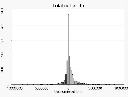
Because the subsequent analysis of this paper frequently uses, either gross or net worth, the distribution of the difference between the two measures for these two wealth concepts are shown in Figures 1 and 2 below. It is possible to reject the null hypothesis that the survey distribution equals the register distribution for these variables. The figures look rather similar though, although debts make the net wealth distribution positively skewed.
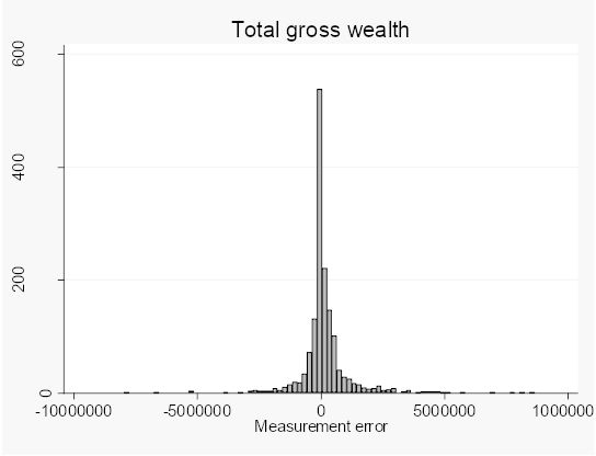
The distribution of the difference between total gross wealth from the SHARE-SE survey and the corresponding register measure from LINDA.

The distribution of the difference between total net worth from the SHARE-SE survey and the corresponding register measure from LINDA.
3. The very rich – estimates of the right tail of the wealth distribution
It is generally believed that a regular sample survey, for instance drawn from a population register, will underestimate the wealth of the very rich mainly because the probability to get them into the sample is rather low and even if they are included, they will choose not to participate. Juster et al. (1999) compared estimates of the wealth distribution from the Panel Study of Income Dynamics (PSID) with those from the Survey of Consumer Finances (SCF). While the former study is a general-purpose household panel survey the latter survey specializes on assets and liabilities and also over-samples the very rich. They found that PSID net worth estimates were not much lower than those from the SCF except in the very last percentile of the distribution.
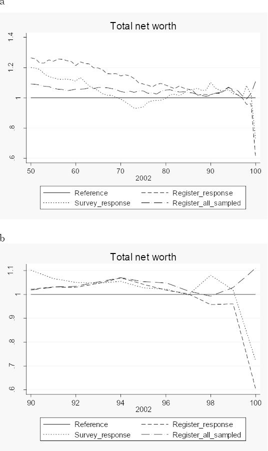
Figure 3 compare the distribution of net worth from the entire LINDA sample for people born before 1953 with the distribution obtained from the UU-RAND sample. The LINDA sample is so large that we for practical purposes can see it as the population. The curves plotted in the figure show ratios of percentile means from the survey to percentile means from LINDA. The three curves differ as to sample coverage and wealth data source. The dotted curve is obtained when the survey responses are used. The dashed curve covers the same sample (those who responded to the survey) but wealth data were taken from LINDA (register data). The dashed-dotted curve finally covers the entire UU-RAND gross sample (including nonresponse) and wealth data were of course taken from registers. The horizontal straight line is the standard of comparison. Figure 3a covers all the percentiles 50-100, while Figure 3b focuses on the richest 10 per cent.

Ratios of total net worth means from the RAND-UU survey to means from LINDA, by total net worth percentiles
One might have expected to see the dashed-dotted curve circle around the straight line, because any difference between the two estimates should only be due to sampling variability. Now, with only one exception this curve stays above the straight line. In the last percentile the survey mean exceeds the LINDA (population) mean by some 10 per cent. The difference between the dashed-dotted curve and the dashed curve comes from nonresponse. We thus find that below the 90th percentile relatively less wealthy people choose not to respond and this kind of selection is largest in the middle of the distribution. However, among the very-very rich the relatively wealthy do not respond. The dashed curve dips in the last percentile. Finally, we find that survey responses underestimate net worth between the 50th and the 85th percentiles but give approximately the same estimates as register data among the very-very rich.8 The survey underestimate in the last percentile is thus due to selective nonresponse but not to under-reporting!
The same analysis was then repeated with the larger SHARE_SE sample. The result is displayed in Figure 4. In this case the two curves using register data dip below the straight line after 95th percentile; the survey response curve is above the straight line almost for the whole plotted distribution and does not dip until the 99th percentile. Up to the 70th percentile there is only a difference in levels between these two curves. Between 90th and 99th percentile the difference between the dashed curve (excluding nonresponse) and the dashed-dotted curve (including nonresponse) is very small suggesting that the impact of nonresponse for these percentiles is low. For the 100th percentile the dashed curve drops below the dashed-dotted curve, again suggesting that the super-rich tend not to respond.
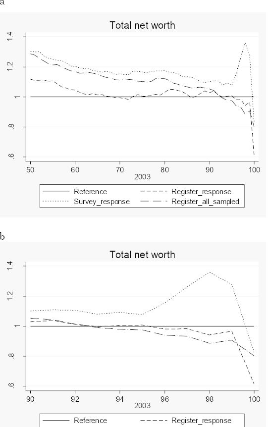
Ratios of total net worth means from the SHARE_SE survey to means from LINDA, by total net worth percentiles
A general conclusion is that the survey data do not give any serious underestimate of net worth with the exception of the very last percentile. We have, however, a small survey and sampling errors may, throw around the estimates in the right tail.
4. Measurement errors in survey data and their consequences
Most of this section assumes that register data give error free estimates, so the measurement error can be defined as the difference between the survey response and the register data. As discussed above this is not a fully realistic assumption, at least not for real property, the market value of which is an error prone estimate also in register data. For these assets we will use the information we have about the error distribution from the data set with purchasing coefficients in an attempt to compensate for these errors in register data. For all other assets we assume that any errors in register data are small compared to those in survey data.
Let us assume the following error structure,
W is the survey measure, the register measure and W* the true value. and are systematic measurement errors and u and ν random errors with zero expectation. In the following we will assume that is zero, an assumption which does not seem very implausible given the properties of financial register data according to the definition of ν in expression (1). It implies that the systematic differences in central tendency between survey and register data we have found in Table 3 are interpreted as systematic measurement errors in survey data.
We do not assume that the random measurement errors are uncorrelated with the true values, but will account for any correlation. For financial assets and liabilities we assume that the variance of ν is zero.
4.1 Measurement errors and the variance (inequality) of wealth
Measurement errors are generally thought to inflate inequality measures. However, this is not necessarily so. From (2a) it follows that,
where S is a standard deviation and ρ a correlation coefficient. If the covariance is negative and large enough to compensate for the variance of u it is even possible that the observed variance underestimates the true variance. For financial assets and liabilities, we can directly compute the moments of eq. (3) from our merged survey and register data, but for real property one also has to use our information about the error structure of register data. From (2b) follows,
For each kind of property all four terms can be estimated from our purchasing coefficient data.9 Assume now that measurement errors in survey data are uncorrelated with the errors in register data. It is not obvious that this is a realistic assumption, in particular if both errors are correlated with the true value, but the two measurement processes are different and not directly related, so we use this assumption as a working hypothesis. It then follows that,
can be estimated from the merged survey-register data, and an estimate of is obtained from the purchasing coefficient data. Eq. (5) thus gives an estimate of Var(u). If we now return to eq. (3) we find that we have estimates of Var(W), Var(W*) and Var(u) and that this equation thus gives us the missing estimate of Cov(W*,u) or the correlation between the survey error and the true value.
For the aggregate assets Other Real Property, Gross Wealth and Net Worth one cannot follow the scheme above. The problem is that the observational unit of the purchasing coefficient data is the sale of a property, not the household. It implies that we cannot get estimates of the covariances between the components of an aggregate. Thus, we can only correct the variance decomposition for Home Equity for errors in register data.
Table 4 gives the statistics needed to evaluate expression (3) for a number of assets. If the entries of the last column had been exactly one the correlation between the true values and the errors had been zero and the classical assumptions had hold true.10 Had they exceeded one the observed variance of the asset had exceeded the true variance by more than under classical error assumptions. We now find that the estimates are smaller than one and that all correlation coefficients are negative. Respondents with small holdings tend to exaggerate them while respondents with large holdings underestimate them. The observed variance is thus smaller than one could have expected from the assumption of classical errors, a result also found in the UU-RAND survey (see Johansson, 2007).
The relative importance of measurement errors in estimating the variance of an asset, by type of asset
| Asset | Var(W) | Var(W*) | Var(u) | A = ρ(W*,u) | B = S(u)/S(W*) | 1+2(A/B) | ||
|---|---|---|---|---|---|---|---|---|
| Own home | 1.03E+12 | 8.50E+11 | 5.95E+11 | |||||
| Own home, corrected | 1.03E+12 | 9.04E+11 | 4.95E+11 | -0.275 | 0.740 | 0.257 | ||
| Other real estate | 2.29E+12 | 2.73E+12 | 1.55E+12 | |||||
| Bank accounts | 5.02E+10 | 4.99E+10 | 1.94E+10 | -0.307 | 0.623 | 0.013 | ||
| Bonds | 1.62E+10 | 2.12E+10 | 8.36E+09 | -0.501 | 0.627 | -0.596 | ||
| Stocks | 1.19E+11 | 1.46E+11 | 8.64E+10 | -0.507 | 0.769 | -0.319 | ||
| Mutual funds | 7.13E+10 | 9.12E+10 | 5.25E+10 | -0.523 | 0.759 | -0.379 | ||
| Debts | 7.02E+11 | 5.45E+11 | 3.04E+11 | -0.180 | 0.746 | 0.517 | ||
| Gross wealth | 2.90E+12 | 2.88E+12 | 1.04E+12 | |||||
| Net wealth | 2.34E+12 | 2.05E+12 | 1.20E+12 |
Although there are relatively large errors in the register-based estimates of the market value of own homes, their influence on the variance decomposition is marginal as a comparison of the first two rows of the table show. The correlation between the survey errors and the true market values is estimated to -0.275. Had we used market values from the registers as “true” the correlation had become -0.291.
In a few cases the observed variance is actually an underestimate of the true variance. This is primarily the effect of rather high negative correlations between errors and true values. For own homes the survey variance exceeds the true variance, because in this case the error variance is relatively large and the negative correlation coefficient of moderate size.
Gross and net wealth is the sum of its components, and the aggregate error is the sum of the errors of the components. The variance of gross (net) wealth becomes a function of the covariances between all true components, between all errors and all covariances between errors and true values. For example, consider an aggregate of just two assets.
Table 5 lists a matrix of variances and correlation coefficients for all combinations we are able to compute. In the main diagonal one finds the variances and in off diagonal elements the correlation coefficients. Looking first at the correlation coefficients between the true components, one finds that most of them are either positive or small. Portfolio diversification suggests that the correlation between risky and less risky assets should be positive. The correlation between the amount in bank accounts and in other assets is positive for all other assets, while the correlation coefficients between bonds and other assets are small and of varying sign.
Variances and correlation coefficients of asset components
| True components | Error components | |||||||||||
|---|---|---|---|---|---|---|---|---|---|---|---|---|
| Own home | Bank | Bonds | Stocks | Mutual Funds | Debts | Own home | Bank | Bonds | Stocks | Mutual Funds | Debts | |
| Own home | 9.04E+11 | -0.275 | ||||||||||
| Bank | 4.99E+10 | 0.081 | 0.244 | 0.406 | 0.100 | -0.307 | 0.264 | -0.078 | -0.091 | -0.019 | ||
| Bonds | 2.12E+10 | -0.005 | 0.104 | -0.050 | -0.013 | -0.501 | -0.027 | -0.090 | -0.050 | |||
| Stocks | 1.46E+11 | 0.265 | 0.096 | -0.222 | 0.072 | -0.507 | 0.218 | 0.026 | ||||
| Mutual Funds | 9.12E+10 | 0.025 | -0.084 | 0.181 | -0.100 | -0.523 | 0.015 | |||||
| Debts | 5.45E+11 | -0.160 | 0.049 | 0.035 | -0.001 | -0.180 | ||||||
| Own home | 4.95E+11 | |||||||||||
| Bank | 1.94E+10 | 0.064 | 0.128 | 0.049 | 0.035 | |||||||
| Bonds | 8.36E+09 | 0.109 | 0.084 | 0.076 | ||||||||
| Stocks | 8.64E+10 | -0.104 | 0.070 | |||||||||
| Mutual Funds | 5.25E+10 | 0.022 | ||||||||||
| Debts | 3.04E+11 | |||||||||||
Turning then to the correlation coefficients between the measurement errors we find that all but one are positive but in most cases rather small.
We have already noted that the correlation between the error and the true value of the same assets is negative and, in most cases, relatively large. Just above half of the error correlations with the true values of other assets are also negative. The inter asset correlations are in most cases much smaller than the intra asset correlations.
The error standard deviation ranges from 39 per cent of the true standard deviation of the same asset (bank holdings and bonds) to about 74 per cent (own home).
We have not been able to estimate the true variances and true error variances of gross and net wealth. All we can do is to compare the survey estimates with the corresponding register estimates. The survey variances only very marginally exceed the register variances (Table 4), and the variance of the difference is about 50 percent of the register variable variance, which implies a correlation coefficient of about -0.23. If the effects of errors in the register-based market values are as small as for own homes we can conclude that without this kind of regression towards the mean in survey responses the observed variances had been much higher.
4.2 Wealth as a dependent variable in regressions
It is often thought that measurement errors in dependent variables are rather innocent. They “only” inflate the error variance by including one extra error component into the variance expression. This is not generally true. It depends on the model structure and functional forms. Even in a very simple linear regression model measurement errors may bias slope estimates. Assume the following simple model,
If W is used instead of the unobserved W* to estimate the model by ordinary least square (OLS), the OLS estimate of becomes,
where is the OLS estimate of the regression slope W* on X and the OLS regression of u on X. Only if the last component is zero in expectation, i.e. the measurement error is uncorrelated with X, becomes an unbiased estimate of .
For financial assets we can directly compute and from our merged survey-register data, but for real property we need to account for the error in register data. The model can also be estimated using register data and we then get an expression analogous to eq. (7),
cannot be computed from purchasing coefficient data because these data do not include the X-variable. Instead assume that plim = 0, then plim = α1. Thus, - consistently estimates plim(buX).
Table 6 gives example estimates of four regression coefficients using age, gender, schooling (years of schooling) and a health measure as alternative explanatory variables. All these variables come from LINDA. Our health measure is an indicator variable which takes the value one if none of the spouses in a family had any income compensated sick days in 2003 and zero if at least one of the spouses had a sickness spell of at least two weeks (The public sickness insurance had a waiting period of two weeks for every sickness spell). Since only employed can obtain sickness benefits and most employees retire at or before the age of 65, our sample in this case reduces to people aged 50-65.
Estimated regression slopes with measurement errors in the dependent variable
| Dep. var | ||||||
|---|---|---|---|---|---|---|
| Indep. var | Age | Gender | ||||
| Own home | -12,654 | -8,821 | -3,833 | -95,289 | -45,449 | -49,840 |
| Other real estate | -5,323 | -1,845 | -3,478 | -130,307 | -210,552 | 80,245 |
| Bank accounts | 1,836 | 2,007 | -171 | -568 | 1,685 | -2,252 |
| Bonds | 557 | 931 | -374 | -1,783 | -2,369 | 586 |
| Stocks | 1,556 | 2,779 | -1,223 | -29,007 | -11,176 | -17,831 |
| Mutual funds | 2,171 | 3,203 | -1,031 | -8,444 | -1,653 | -6,791 |
| Debts | -15,877 | -10,968 | -4,910 | -105,990 | -122,514 | 16,525 |
| Gross wealth | 27,129 | 21,292 | 5,837 | -113,586 | -153,823 | 40,236 |
| Net wealth | 43,006 | 32,260 | 10,747 | -7,597 | -31,308 | 23,711 |
| Schooling | Health | |||||
| Own home | 64,900 | 57,997 | 6,903 | 71,591 | 105,627 | -34,035 |
| Other real estate | 40,892 | 21,286 | 19,606 | 150,175 | 124,325 | 25,850 |
| Bank accounts | 1,330 | 561 | 769 | 24,508 | 25,349 | -841 |
| Bonds | -805 | -2,747 | 1,942 | 12,991 | 5,489 | 7,501 |
| Stocks | 3,210 | 3,791 | -581 | -6,888 | -7,140 | 253 |
| Mutual funds | 6,056 | 3,677 | 2,379 | 50,412 | 50,437 | -24 |
| Debts | 91,571 | 35,350 | 56,221 | 4,049 | -41,256 | 45,305 |
| Gross wealth | 152,642 | 108,158 | 44,484 | 474,173 | 188,870 | 285,303 |
| Net wealth | 61,071 | 72,808 | -11,737 | 470,124 | 230,126 | 239,998 |
Several of the entries in Table 6 show that the regression of the measurement error on the explanatory variable deviates much from zero, which implies that the survey measure grossly over or underestimate the marginal effect of the explanatory variable. For instance, the age effect on net wealth is overestimated by 33 percent, the schooling slope is overestimated by a factor of 2.6 and the effect of not being sick is overestimated by more than 100 percent. There are also examples of large negative regressions of the error on the explanatory variable. For instance, the survey error of the market value of own home is negatively related to age, gender and health, which implies that the survey underestimates the corresponding slopes. In summary, many of these examples suggest that we risk a relatively large bias due to correlation between the measurement error and the explanatory variable.
4.3 Wealth as explanatory variable in regressions
Assume the same measurement error model as above but now consider using W* as an explanatory variable in an OLS regression. Then the structural model is,
Y could for instance be bank holdings and W gross wealth. Then this model could be viewed as a very simple portfolio choice model. In Table 7 different types of assets will be used as Y variables to see if the impact of measurement errors in gross wealth is different across assets. Thus, in this section and the next W* is equal to gross wealth irrespectively of Y variable. If W* is replaced with the error prone survey variable W when eq. (9) is estimated by OLS, we obtain
Estimated regression slopes with measurement errors in the independent variable (gross wealth)
| Dep. Var. | * | * | * | /* | ||
|---|---|---|---|---|---|---|
| Own home | 0.277 (0.013) | 0.310 (0.011) | -0.159 | 1.20E+12 | 3.32E+12 | 0,360 |
| Other real estate | 0.521 (0.028) | 0.634 (0.018) | -0.544 | 2.01E+12 | 5.72E+12 | 0,352 |
| Bank accounts | 0.045 (0.003) | 0.047 (0.003) | -0.002 | 9.70E+11 | 2.95E+12 | 0,328 |
| Bonds | 0.000 (0.004) | 0.002 (0.004) | -0.007 | 1.69E+12 | 6.80E+12 | 0,249 |
| Stocks | 0.039 (0.006) | 0.047 (0.006) | -0.028 | 1.76E+12 | 4.70E+12 | 0,376 |
| Mutual funds | 0.057 (0.005) | 0.055 (0.005) | 0.000 | 1.31E+12 | 3.89E+12 | 0,336 |
| Debts | 0.263 (0.012) | 0.272 (0.011) | -0.001 | 1.91E+12 | 6.27E+12 | 0,304 |
| Health | 1,55E-08 (9,15E-09) | 1,68E-08 (1,03E-08) | -1,19E-01 | 1,1E+12 | 2,14E+12 | 0,505 |
-
*
Computed as if there were no errors in register data.
Using the assumptions of eq. (9) the second term to the right of the equality sign in (10) vanishes in probability when the sample size tends towards infinity. Thus,
If measurement errors in survey data have so called classical properties, plim(buW*) = 0, and we get the traditional textbook case with a downward bias. However, if measurement errors are correlated with the true values this correlation can compensate for the error variance and reduce the bias. For instance, if the ratio of the two error variances is 0.5 and buW* = -0.5, then the estimator is consistent! Table 4 gives implicitly estimates buW* and variance ratios for most assets, but not for gross wealth. For gross wealth we do not have the information needed to compute the variance ratio and the regression of the measurement error on the true value. If the survey measure is replaced by the register counterpart, we get an OLS estimator with the same structure as in eq. (10) and (11) but with the survey error u replaced by the register data error ν. Because this error only comes from the market value estimates of real property while financial assets and debts are considered error free, one might believe that the ratio of the error variance to the true variance and the regression coefficient of the error on the true value are smaller in this case than for survey data. Table 7 compares slope estimates using survey and register gross wealth as an explanatory variable in a number of regressions with register asset variables and a health variable as dependent variables. The table also gives buW* coefficients and variance ratios computed as if there were no errors in register data. These statistics are not the same in every row because the samples are not the same. Every regression was run only for those who had a nonzero dependent variable in the survey. We might note that the error regression slope coefficient varies a great deal depending on the sample used.
For all cases but for mutual funds and debts the survey-based estimates are smaller than the register based, suggesting that the bias component is larger in survey data than in register data in most of the cases. But this is a conclusion which is not justified. Assume, for instance that the error regression slope in register data is -0.16 and the ratio of the error variance to the true variance is 0.1, then register data will overestimate by 7.7 percent.
The discussion above assumed that there were no measurement errors in Y. However, if we regress real properties from register data on gross wealth both the dependent variable and the explanatory variable are error prone. We then have to modify eq. (11) by adding plim(bνW*) to the numerator,
This result rests on the assumption that measurement errors in the survey are uncorrelated with those in register data.
Finally, if both the asset variable and gross wealth come from the survey, the probability limit of the slope estimator is given by eq. (12) if plim(bνW*) is replaced by plim(), where ui is the measurement error of the i:th asset.
It is difficult to draw any general conclusions about the effect of measurement errors in the independent variable from this exercise with the limited information available. Judging just from the relative error variances in survey data in Tables 4 and 7 one might believe that we would tend to underestimate the slope coefficient by approximately 30 percent, but a negative correlation between errors and true values reduces this bias considerably. Small variations in this correlation and in the variance ratio can change the bias in the slope estimate a great deal. Judging from the rather close agreement between the survey and register estimates in the first two columns of Table 7 one might however conjecture that measurement errors in the explanatory variable gross wealth are rather innocent.
4.4 Wealth as explanatory variable in regressions with one additional X-variable
Let’s now add another explanatory variable to model (9).
It is estimated by OLS using observable W substituted into (13b). This model could be viewed as a slightly more realistic portfolio choice model. In terms of second order moments the multivariate OLS estimates of the slope parameters become,
and
From expression (15) follows the well-known result that even if the measurement error is uncorrelated with all other variables is a biased estimate of . In general, the bias will depend on all correlations between u and other variables. Table 8A–8C give estimates of the relation (13b) with each asset from registers as dependent variable and using the register gross wealth measure () and alternatively the survey measure (W) jointly with three alternative additional explanatory variables. In Table 8A it is the age of the main respondent in the household,11 in 8B it is the gender of the main respondent, and in 8C it is the years of schooling of the main respondent. These tables also give the second order moments needed to evaluate the expression (15) and the analogous expression for (14) not written out explicitly.
Multivariate regressions with errors in one explanatory variable and decomposition of the estimates.
| Dep. Var | |||||||||||||
|---|---|---|---|---|---|---|---|---|---|---|---|---|---|
| A. Explanatory variables are gross wealth (W) and age (X) | |||||||||||||
| Own home | 0.275 (0.013) | -4,727 (2,335) | 0.309 (0.011) | -6,265 (2,129) | 0.360 | 0.310 | -8,821 | -2.29E-07 | -5.08E-07 | -0.224 | -8,274 | -6,608 | -0.159 |
| Other real estate | 0.524 (0.028) | 9,204 (6,906) | 0.635 (0.018) | 6,545 (4,763) | 0.352 | 0.634 | -1,845 | -1.87E-07 | -3.17E-07 | -0.252 | -13,219 | -7,869 | -0.544 |
| Bank accounts | 0.048 (0.003) | 3,033 (559) | 0.048 (0.003) | 2,703 (556) | 0.328 | 0.047 | 2,007 | -5.37E-07 | -8.16E-07 | -0.154 | -14,374 | -7,173 | -0.002 |
| Bonds | 4.7E-04 (0.004) | 946 (1,013) | 2.1E-03 (0.004) | 971 (1,007) | 0.249 | 0.002 | 931 | -2.81E-07 | -7.00E-07 | -0.175 | -19,656 | -12,194 | -0.007 |
| Stocks | 0.041 (0.006) | 3,857 (1,367) | 0.048 (0.006) | 3,398 (1,332) | 0.376 | 0.047 | 2,779 | -2.30E-07 | -6.40E-07 | -0.217 | -12,905 | -13,479 | -0.028 |
| Mutual funds | 0.060 (0.005) | 4,353 (987) | 0.056 (0.005) | 3,814 (990) | 0.336 | 0.055 | 3,203 | -2.74E-07 | -6.29E-07 | -0.188 | -10,888 | -8,387 | 0.000 |
| Debts | 0.268 (0.012) | -13,469 (3,154) | 0.276 (0.011) | -16,554 (2,970) | 0.304 | 0.272 | -11,846 | 2.45E-07 | -5.79E-07 | -0.173 | 17,004 | -10,959 | -0.093 |
| B. Explanatory variables are gross wealth (W) and gender (X, female=1) | |||||||||||||
| Own home | 0.277 (0.013) | 3,397 (44,761) | 0.310 (0.011) | 1,396 (40,964) | 0.360 | 0.310 | -45,449 | -1.14E-08 | -5.27E-09 | -0.224 | -150,951 | -25,189 | -0.159 |
| Other real estate | 0.520 (0.028) | -128,274 (124,484) | 0.633 (0.018) | -126,637 (85,960) | 0.352 | 0.634 | -210,552 | -5.76E-09 | -3.17E-09 | -0.252 | -132,611 | -25,710 | -0.544 |
| Bank accounts | 0.046 (0.003) | 16,355 (11,825) | 0.047 (0.003) | 13,305 (11,761) | 0.328 | 0.047 | 1,685 | -2.08E-08 | -1.94E-08 | -0.154 | -245,958 | -75,333 | -0.002 |
| Bonds | -6.6E-05 (0.004) | -2,407 (20,194) | 1.8E-03 (0.004) | -1,331 (20,176) | 0.249 | 0.002 | -2,369 | -2.14E-08 | 1.56E-09 | -0.175 | -594,537 | 10,801 | -0.007 |
| Stocks | 0.039 (0.006) | 3,417 (25,094) | 0.047 (0.006) | -1,385 (24,489) | 0.376 | 0.047 | -11,176 | -1.11E-08 | -2.36E-08 | -0.217 | -207,620 | -166,465 | -0.028 |
| Mutual funds | 0.058 (0.005) | 11,990 (19,698) | 0.055 (0.005) | 9,434 (19,756) | 0.336 | 0.055 | -1,653 | -1.29E-08 | -6.85E-09 | -0.188 | -200,887 | -35,733 | 0.000 |
| Debts | 0.266 (0.013) | -37,655 (49,847) | 0.272 (0.011) | -80,012 (47,078) | 0.304 | 0.272 | -148,691 | -1.52E-08 | -3.62E-08 | -0.173 | -252,850 | -164,188 | -0.093 |
| C. Explanatory variables are gross wealth (W) and year of schooling (X) | |||||||||||||
| Own home | 0.260 (0.013) | 27,887 (5,737) | 0.297 (0.011) | 29,504 (5,159) | 0.360 | 0.310 | 57,997 | 4.62E-07 | 2.63E-07 | -0.224 | 96,035 | 19,657 | -0.159 |
| Other real estate | 0.539 (0.029) | -43,158 (15,410) | 0.645 (0.018) | -40,365 (10,456) | 0.352 | 0.634 | 21,286 | 2.81E-07 | 2.01E-07 | -0.252 | 95,603 | 24,045 | -0.544 |
| Bank accounts | 0.049 (0.004) | -5,824 (1,538) | 0.049 (0.003) | -4,135 (1,504) | 0.328 | 0.047 | 561 | 5.16E-07 | 5.60E-07 | -0.154 | 95,628 | 34,094 | -0.002 |
| Bonds | 0.002 (0.004) | -3,073 (2,584) | 0.003 (0.004) | -3,115 (2,493) | 0.249 | 0.002 | -2,747 | 3.20E-07 | 6.48E-07 | -0.175 | 132,626 | 66,831 | -0.007 |
| Stocks | 0.040 (0.006) | -1,698 (3,200) | 0.048 (0.006) | -1,112 (3,077) | 0.376 | 0.047 | 3,791 | 3.60E-07 | 3.24E-07 | -0.217 | 103,054 | 34,823 | -0.028 |
| Mutual funds | 0.059 (0.005) | -3,609 (2,474) | 0.056 (0.005) | -1,431 (2,444) | 0.336 | 0.055 | 3,677 | 4.00E-07 | 3.98E-07 | -0.188 | 91,814 | 30,697 | 0.000 |
| Debts | 0.268 (0.013) | -1,819 (6,867) | 0.271 (0.012) | 3,953 (6,444) | 0.304 | 0.272 | 33,058 | 3.58E-07 | 2.79E-07 | -0.173 | 107,231 | 22,858 | -0.093 |
-
Note: In computing these statistics u was defined as .
For all assets but mutual funds and debts we again find that the slope estimate of the gross wealth variable is smaller when survey data are used compared to register data. With the exception of real property there are, however, no large differences. The estimates differ for real property primarily because of the relatively large (in an absolute sense) regressions of the dependent variables on the measurement errors for these two assets, see the last column of Table 8A–C. For bonds and for mutual funds this regression coefficient is zero or virtually zero. These results hold independently of supplementing X-variable. The partial effects of the X-variables are estimated with relatively large errors and we do not consistently find positive of negative differences in slope estimates.
5. Conclusions
Surveys tend to underestimate total net worth among the very-very rich – the top 1 per cent. Our results suggest that this is due to selective nonresponse, but not to underreporting among those who participate in the survey. The wealthiest among the very-very rich do not participate in the survey, Below the top 1 per cent our two surveys give different results. The UU-RAND survey suggests that households with relatively low wealth tend to drop out while the SHARE-SE survey suggests the opposite, and in UU-RAND participants tend to underreport, while they over-report in SHARE-SE.
The main problem with measurement errors in surveys of household wealth is not that surveys systematically underestimate wealth – this study rather suggests that they overestimate net worth and most of its components - but the large variance of the error distribution and the correlation between errors and true values. There is a strong negative correlation between errors and true values implying that rich households tend to underreport while poor households over-report their assets.
The error variance ranges from almost 40 per cent of the true variance for bank holdings to almost 60 per cent for stocks, and the correlation between error and true value from -0.17 for debts to -0.52 for mutual funds. These large negative correlations imply that measures of inequality do not become inflated in surveys. Surveys might even underestimate inequality.
Measurement errors in survey responses to questions about assets are not only correlated with the true values but also with standard explanatory variables such as age, gender and schooling. This implies that not only in models where wealth is an explanatory variable will we get biased estimates of model parameters but also in models which have wealth as a dependent variable. Our results show that when we run regressions of assets on age, gender, schooling or health we in many cases get large differences between survey and register data because the measurement errors are correlated with the explanatory variable. The bias introduced is not consistently positive or negative. The sign depends on the combination of dependent and explanatory variables. Judging from these examples, however, so called classical assumptions only hold exceptionally.
When error prone gross wealth is used to explain error-free assets the negative bias from the error variance as such is to a large extent compensated by the negative correlation between the errors and the true values. The result is that the survey estimate of the marginal effect of gross wealth appears to have little bias. The same result continues to hold when one of three exogenous variables is added to the model.
In summary, it is obvious that measurement errors in wealth surveys do not have so called classical properties and that they can seriously distort conventional analysis of the wealth distribution as well as bias estimates of model parameters when wealth or single assets enter a model on either side of the equality sign. However, the negative correlation between measurement errors and true values tend to compensate for the relatively large error variance and give survey estimates of inequality and of the marginal effect of wealth that are not very far off. But getting descent estimates for the wrong reason is a poor consolation. It is therefore important that we continue to learn more about the properties of these errors so they can be built into our models, and we can learn how to compensate for measurement errors.
Footnotes
1.
2.
Before the 1992 income tax reform it was common that the person with the highest income was registered for mortgages and loans. To some extent this practice might extend today.
3.
”Did you or your spouse….?”
4.
5.
However, note that if the property is not declared the owner cannot deduct interest paid on any mortgage on the property.
6.
These data include property owned by people independently of the owner’s age. Ideally we should have limited the data set to properties owned by those who were 50+, but there is no information about the owner included in the data set.
7.
Descriptive statistics for the UU-RAND survey can be found in Johansson (2007). The conclusions from the descriptive statistics for the SHARE_SE survey also hold for the UU-RAND survey.
8.
The upturn of the dotted curve at the 98th percentile is due to a few households having reported very large assets.
9.
10.
The classical assumption assume that measurement errors are uncorrelated with the true values, the true value of other variables included in the model, and any errors in those variables including the stochastic disturbance term.
11.
The main respondent is the individual sampled to identify the household.
References
-
1
The Handbook of SESIM – a Swedish Dynamic Micro Simulation ModelMinistry of Finance, Economic Policy and Analysis Department.
-
2
Essays on Measurement Error and Nonresponse, Economic Studies No 103Uppsala: Department of Economics, Uppsala University.
-
3
Explaining the Size and Nature of Response in a Survey on Health Status and Economic Standard, J of Official Statistics, Vol. 24, No 3, Pp 431-449Explaining the Size and Nature of Response in a Survey on Health Status and Economic Standard, J of Official Statistics, Vol. 24, No 3, Pp 431-449.
-
4
The measurement and structure of household wealthLabour Economics 6:253–275.https://doi.org/10.1016/S0927-5371(99)00012-3
-
5
The Survey of Health, Ageing and Retirement in Europe. MethodologyThe SHARE Sampling Procedures and Calibrated Design Weights, The Survey of Health, Ageing and Retirement in Europe. Methodology, Mannheim, Mannheim Research Institute for the Economics of Ageing.
Article and author information
Author details
Funding
No specific funding for this article is reported.
Acknowledgements
This article has been originally published as Chapter 2 in Fredrik Johansson (2007) Essays on Measurement Error and Nonresponse, Economic Studies 103, Department of Economics, Uppsala University, ISBN 978-91-85519-10-1. We acknowledge the access to the SHARE wave one data and register data from Statistics Sweden. The views expressed in the article belong solely to the authors, and not to the National Institute of Economic Research.
Publication history
- Version of Record published: April 30, 2022 (version 1)
Copyright
© 2022, Johansson and Klevmarken
This article is distributed under the terms of the Creative Commons Attribution License, which permits unrestricted use and redistribution provided that the original author and source are credited.