Modeling Work Incentives in Microsimulation Models
- Department of Economics, Sweden
1. Introduction
According to my Oxford dictionary an incentive is: "that which incites or arouses a person to action" (incite = encourage). Work incentives have to be assumed, modeled, tested, estimated and put into a microsimulation model. By using a microsimulation model we can analyze the effects of the work incentives we have included in the model but the incentives as such cannot be analyzed by the microsimulation model.
What incites a person to work or not to work? Is another child an incentive to work or not to work? There are results which show that both men and women, but in particular women, adjust their hours of work when they get another child. Women decrease their hours. The size of the adjustment depends for instance, on the education and labor market attachment of the woman and on the eligibility to and replacement rate of maternity and family allowances. For men there are conflicting results. In Sweden there are indications that also men, at least some men, also decrease their hours, but there are also results, in particular for other countries which suggest that married men with children work very long hours.
Some microsimulation models do capture some of these incentive effects of children on work, but it is not what I would like to discuss. I would rather like to concentrate on those incentives which lie in the core of most microsimulation models, on those incentives which a microsimulation model has a relative advantage in computing, i.e. the incentives from taxes and benefits. The advantage of a microsimulation model compared to alternative approaches is its capacity to compute with great detail the taxes and benefits which fall upon a household. Many other economic models only use stylized tax and benefit systems which might distort the analyses, but in microsimulation models one can include all the details and use the policy parameters actually used by the politicians. An average marginal tax rate is not a policy instrument but the definition of the tax base is (incl. deductions, thresholds etc.), and the location of the kink points which define tax brackets and the tax rates as such are policy instruments. In evaluating the incentive effects all these details should be used and a microsimulation model is a good instrument for doing it.
Furthermore, many microsimulation models has as their main objective to analyze the effects of tax and benefit changes on the income distribution, but few models include the behavioral adjustments which follow from new tax and benefit incentives.
To include these behavioral adjustments we need a model which explains how new incentives result in new work behavior. The key issue is thus, how we should model the behavioral adjustments, which follow from changes in taxes and benefits.
I would now like to make a few quick observations:
There is certainly no single approach to solve this problem, many approaches could give satisfactory results depending on the circumstances.
The approach chosen would most certainly depend on what tax and benefit changes we are talking about and on how we choose to define work.
Modeling behavior is not a problem which is unique to microsimulation and the solution should probably not be sought as a specific microsimulation-solution. On the contrary, this is a problem which has been analyzed by labor economists for decades and no microsimulation model is likely to be better than economic research in the area,
however, microsimulation models have certain objectives, in particular to simulate well the distributions of hours, earnings and income, which might suggest certain approaches. Microsimulation also have certain advantages, which I have already mentioned, and certain characteristics from which one should benefit.
In the following I would like to share with you certain ideas about how one could approach this problem. I have not done any empirical studies of my own, what I have is more like a research agenda. But let us first look into a few already existing models to find out how work incentives have been handled in these models.
2. Work incentives in already existing microsimulation models: a few examples and potential extensions
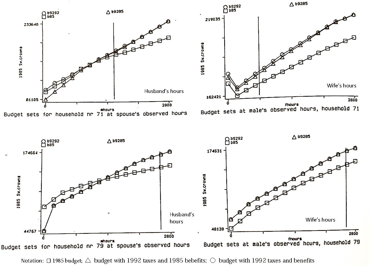
Most static tax-benefit models like the Danish Law Model and the Swedish Fasit have no behavioral adjustments effects at all, but they can be used to compute statistics which might be indicative of behavioral adjustments. For instance, in many models the marginal tax rate or the composite marginal effect of taxes and benefits is the key measure of work incentives, and a static tax-benefit model can be used to compute marginal effects for various groups of individuals. If they are large, one might also expect large behavioral adjustments. We have been used to see diagrams of marginal effects as a function of income, but the marginal effect is just the slope of the budget set, and it might be useful to visualize the whole budget set. Figures 1–3 illustrates how this could be done. These diagrams are borrowed from Klevmarken et al. (1995). The two top diagrams in Figure 1 gives the budget sets with the 1985 and 1992 tax systems for a couple. In the left diagram the budget set is a function of the husbands work hours and in the right diagram a function of the spouse’s work hours. In the first diagram the spouse’s hours are kept at their observed number and in the second diagram the husband’s hours are at their observed number. The vertical line marks the observed hours for the husband and wife respectively. The diagrams show that the introduction of the new tax system increased after tax income, and if the husband would increase his hours, he would have gained more from the new system than the old, while the spouse’s gain if she would increase her work hours is not much greater with the new system compared to the old. The second pair of diagrams in Figure 1 shows the budget sets for another couple.

Budget sets for two households by husband’s and wife’s workhours. Source: Klevmarken et al. (1995) Figure 2.7.

Median Budget sets for single women 1985 with 1985 taxes and benefits and with 1992 taxes and 1985 benifits respectively. Source: Klevmarken et al. (1995) Figure 2.8.

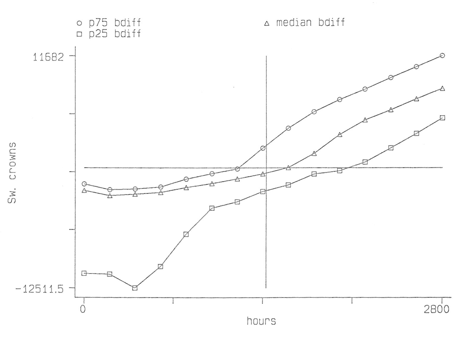
Quartile changes in disposable income by workhours for single women caused by the taxchanges 1985-92. Source: Klevmarken et al. (1995) Figure 2.11.
If one is working with a large sample, it is of course impossible to draw diagrams for all sample members. They need be summarized. Figure 2 shows the median budget sets for single women. In this case the vertical line marks the mean hours of work. At this number of hours there is not much change in median income as a result of the tax change, but the marginal return of a change in work hours is a little higher (in the median) in the new tax system. This diagram is, however, a little deceptive because it hides the great variability in the budget sets. This is illustrated in Figure 3 which shows the gain in income from the tax change. The top curve is the third quartile, the middle curve the median and the bottom curve the first quartile gain. The horizontal line marks the zero point and the vertical line the mean number of hours worked. We find, for instance, that a little less than 50 per cent of single women, who worked at the mean hours, gained from the tax reform, and that about three quarters of those who worked full time gained, while most of those who worked half time lost in income.
Let us now turn to dynamic models and start with DYNASCAN the Canadian adaptation of the US model CORSIM. The only explanatory variables used in two probit equations for weeks worked are age, education, marital status and the unemployment percentage. There are thus no tax or benefit incentives at all in this model (DYNASCAN, 1995)
In the logit model for exits to unemployment in the Australian model DYNAMOD (monthly transition rates) the explanatory variables are demographic variables, occupational indicators and a few aggregate variables like the unemployment rate, average weekly earnings and the ratio of maximum weekly rate of unemployment benefits to the average weekly earnings in the public sector. There are thus no personal tax or benefit incentives built into this equation either. ( Antcliff et al., 1996, Page 196, Table 3.)
CORSIM, DYNASCAN and DYNAMOD all use relatively simple transition probability functions which in general cannot be derived from a structural model of economic behavior. To include the incentive effects of taxes and benefits on work we need a structural model, which shows how decisions are made and how they are influenced by the true policy parameters. The Swedish model MICROHUS, Klevmarken and Olovsson (1996), does not go all the way but some distance in this direction.
The econometric model used for the transition into the labor force is a Weibull proportional hazard model. In addition to variables like age, schooling and labor market experience, there are three income variables attempting to capture incentive effects. They are the income an individual would obtain after tax if he/she did not work at all, if he/she worked half-time or full-time. These variables interact with age dummies and a pension dummy to make it feasible to differentiate the incentive effects by age and by pension status. The larger the potential income from full-time work is, the higher probability to take up work, in particular for males older than 30 years. The estimates for females were insignificant.
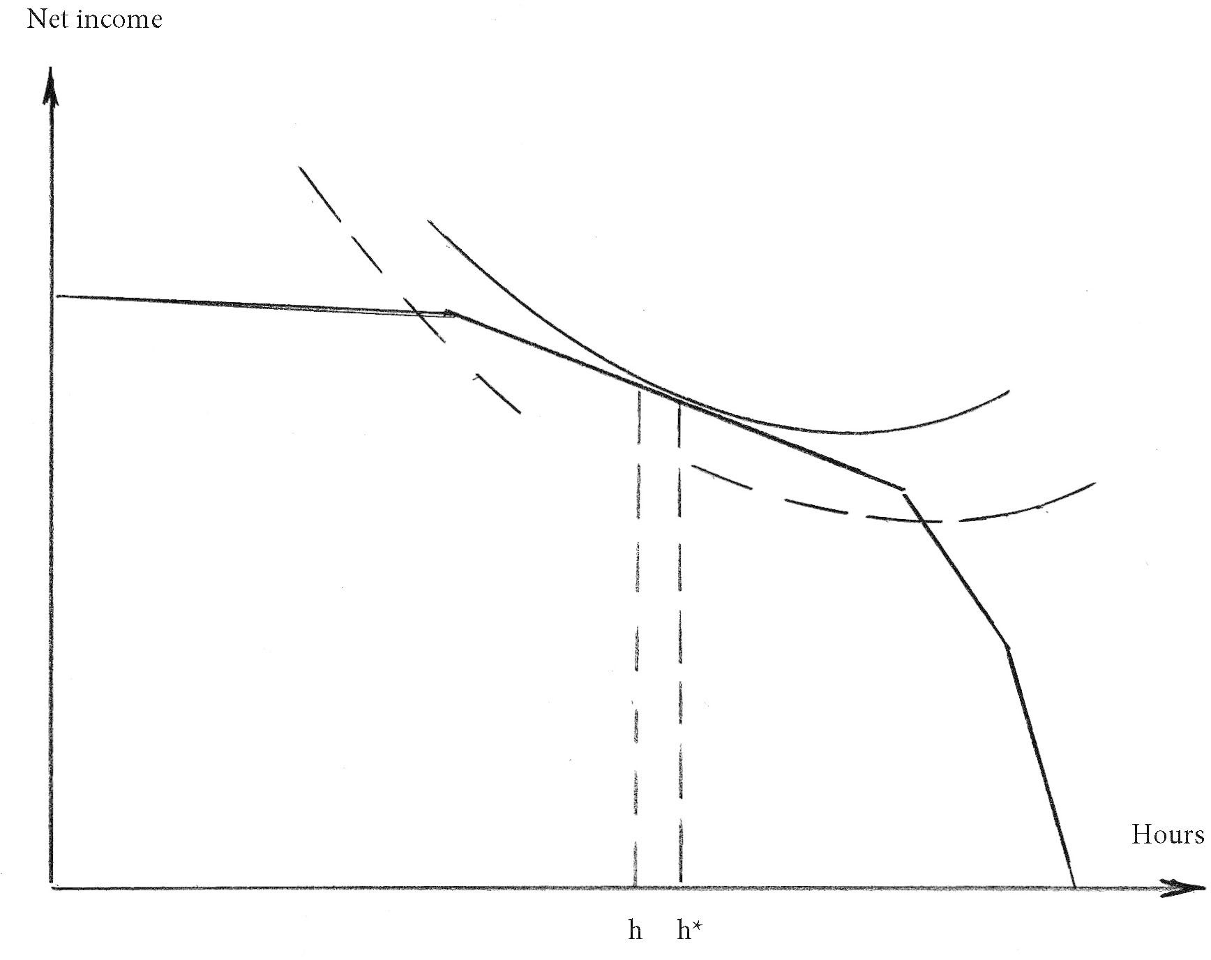
MICROHUS uses a Hausman model to simulate hours of work given that an individual is in the labor force and not unemployed. The idea behind the Hausman model is illustrated in Figure 4. Along the horizontal axes we mark hours of leisure and along the vertical axis income after tax. The convex piece wise linear curve shows the budget set of an individual with a progressive tax system. The slope of the curve becomes smaller the more the individual works, and the higher his income and marginal tax rate becomes. (A move towards the income axis.) An indifference curve has a point of tangency to the budget set at h* hours, which is the optimal "desired" number of hours for this individual. We do not observe h* but h because it might not have been possible to find a job at h* or there might be measurement errors in our measure of hours of work. The deviation h*-h is usually assumed to be random and normally distributed. The estimates of the wage rate and income elasticities used in MICROHUS are reproduced in Table 1. All income elasticities are negative. As income increases singles decrease their work hours more than married and cohabiting couples. In the latter group males react marginally stronger than females. All compensated wage rate elasticities are positive and the elasticity for singles is much higher than those for married and cohabiting males and females.

Budget set and indifference curves.
Estimated wage rate and income elasticities from a Hausman model in MICROHUS.
| Elasticities* | Singles | Males | Females |
|---|---|---|---|
| Wage rate | 0.1433 | -0.0132 | -0.0057 |
| Income | -0.5813 | -0.1813 | -0.1493 |
| Compensated | 0.6011 | 0.1296 | 0.1119 |
-
*
Note: The last two columns include estimates for married and cohabiting couples.
The advantages and disadvantages of the standard Hausman type of labor suppiy model has been discussed at some length in the labor supply literature. I am not going to repeat this discussion now, but refer, for instance, to the "Rockwool Report", Atkinson and Mogensen (1993). I would rather like to stress three shortcomings which are of particular relevance for microsimulation:
The Hausman model does not predict well the distributions of hours, and if a microsimulation model does not, then the simulation of the income distribution is likely to become bad too. This is illustrated in Figure 5 and Figure 6 which are borrowed from van Soest et al. (1990).
The model assumes that each individual takes a new decision about his/ her labor supply every year and that this decision is independent of last year’s decision. The model is also typically estimated from cross-sectional data. The implication is that this model, used in a microsimulation model, will simulate an excessive mobility in hours. (If we are only interested in cross-sectional distributions, we might be able to live with this property, but if we are interested in mobility or life-cycle incomes then we cannot.)
The model gives the behavior of a single individual, while the decision unit is typically a household or a family. The decisions made of two spouses are certainly not independent. This is also of particular importance in a microsimulation model because we are frequently interested in the income standard of households or the adult equivalent income distribution which is obtained by dividing household income by some equivalence scale. If we do not get the correlation between husband’s and wife’s work hours correct, we are not likely to get household income right either.
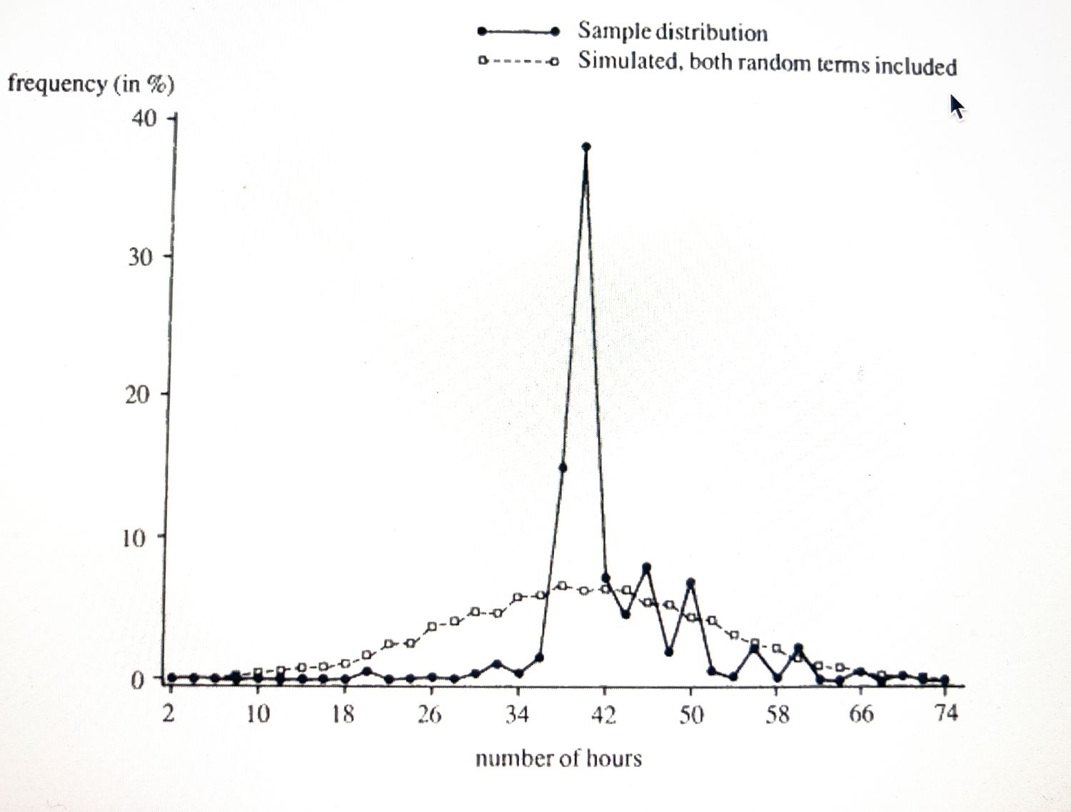
Distribution of working hours, males. Simulated values from a Hausman model. Source: van Soest et al. (1990).

Distribution of working hours per week, females. Simulated vales from a Hausman model. Source: van Soest et al. (1990).
The first and the last of these three problems have been discussed and dealt with in the literature.
The Dutch microsimulation model NEDYMAS (Nelissen, 1994) uses a model which solves the first problem. (A similar approach was used by Dagsvik (1988), Dagsvik and Ström (1988), Ljones and Ström (1987), Anderson et al. (1988) and Aaberge, et al. (1990) ) Dagsvik (1988) Dagsvik & Ström (1988) Ljones & Ström (1987) Aaberge et.al. (1989).
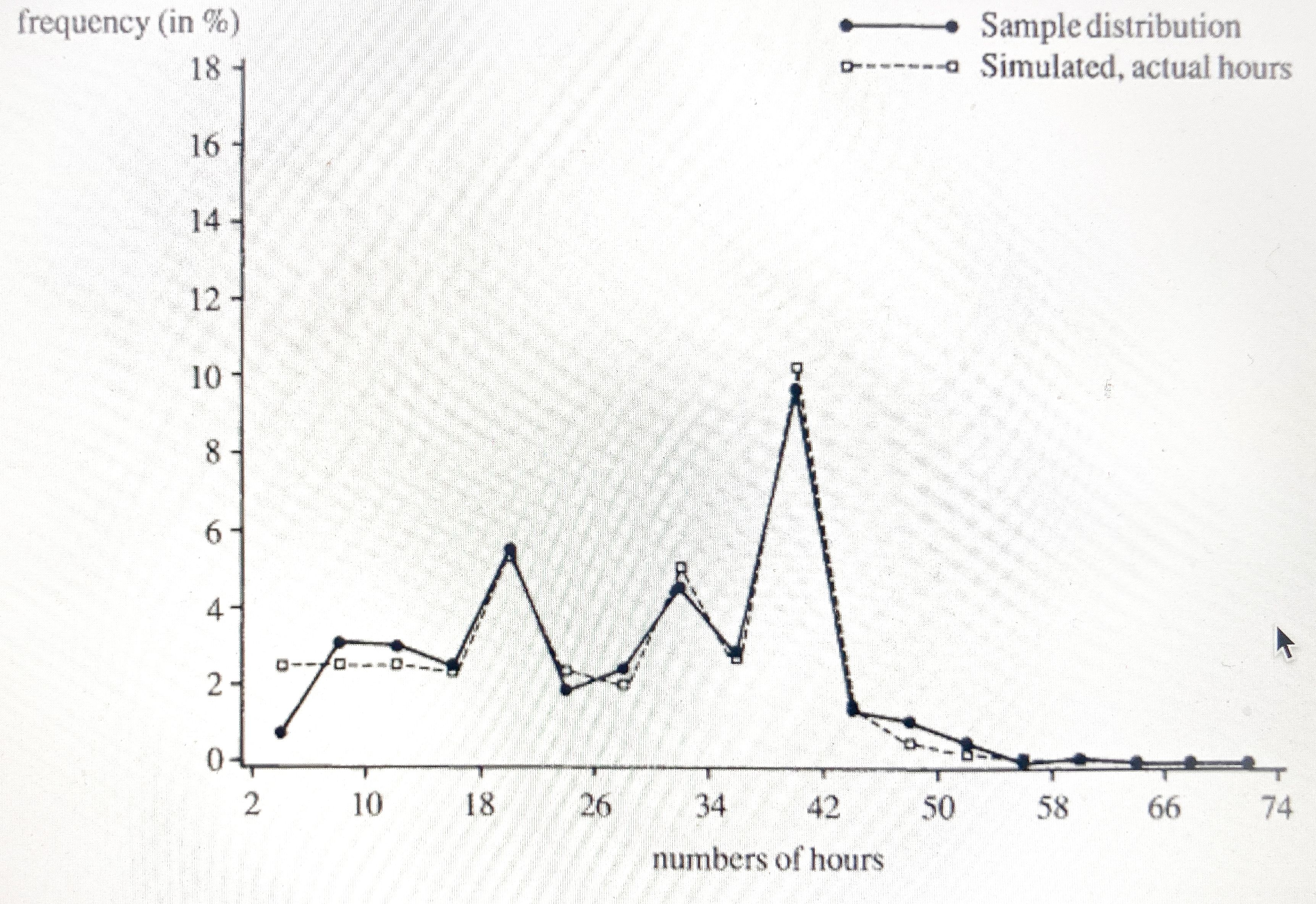
The idea is that the sharp peaks of the hours distribution come from restrictions on the demand side. Jobs are usually only offered with certain hours of work, and individuals who do not get offers with their desired hours will have to choose among second-best alternatives. If job offers are drawn from a distribution of hours which has the characteristic peaks, then the simulated distribution of work hours will have them as well. This principle is illustrated in Figure 4. Assume that no offer is obtained with h* hours of work but two offers, indicated by the intersections of the budget set and the two dashed indifference curves. The individual will then have to evaluate which of these two alternatives will give him the highest utility and choose accordingly (unless no work gives even higher utility) Nelissen (1994) estimated the parameters of the offer distribution subject to identifying assumptions. Their model was now able to predict the observed distributions of hours worked, see Figures 7 and 8. In order to rely less on identifying assumptions one would ideally like to have data on job offers and/or desired hours, not only hours actually worked (or contracted).

Distribution of working hours per week, males. Simulated hours from a model including offered hours. Source: van Soest et al. (1990), Figure 2.

Distribution of working hours per week, females. Simulated values from a model including offered hours. Source: van Soest et al. (1990).
One could think of the number and type of job offers to an individual as a function of the vacancy (or unemployment) rate and other demand indicators as well as individual characteristics (occupation, industry, age, gender, schooling and search effort etc.)
If an individual do not get any job offers or if he chooses not to accept any of those he receives, he becomes unemployed (or leaves the labor force). By allowing the parameters of the offer distribution to depend on factors which are related to vacancies or unemployment it is possible to introduce a heterogeneity in the risk of becoming unemployed. There is, however, a remaining problem with timing. The budget set of a Hausman model is usually an annual budget set because taxes are computed on an annual basis, but a person might become unemployed at any time in a year. A mechanism is thus needed which dates the transition from employment to unemployment. (One reason for this is that unemployment compensation is given on a daily basis.) One possibility is to draw a date randomly, another to allow job offers to arrive sequentially every day or every week and scale down the probability of exits to unemployment to daily or weekly probabilities. It is, however, not obvious how such a mechanism could be made consistent with utility maximization subject to an annual budget constraint.
Another possibility to develop the model further is to introduce a memory into the model, and thus solve the second problem in my list by assuming that everyone who is employed gets an offer to keep his/her job with a high probability. This probability could be made a function of the vacancy or unemployment rate and of personal characteristics, and thus vary both across individuals and over time. In this way most individuals will keep their old jobs and work hours, but some will become unemployed unless they get another job offer and accept it, and some will accept new job offers although they already have a job. To estimate such a model one will need annual panel data with at least two observations on each individual. The possibility to identify and estimate both preference parameters and offer distributions will depend on what 6 specific assumptions are made and what kind of data are available.
Solutions to the third problem suggested in the literature are either to assume a household "utility function" which is maximized subject to a household budget set or to use a game-theory approach.
At least the first of these approaches could probably be used within the modeling framework I have been discussing. One would then need to model job offers to both spouses, and the issue of dependence or independence of their offers arises.
The model could also be generalized in another way. Jobs are not only characterized by their hours of work but also by a wage rate, fringe benefits and other work conditions. More generally, the compensation for a job could be given in the form of a flat hourly wage rate, a monthly salary or some kind of incentive scheme. With a job could also follow the opportunity to do over time, or the obligation to do it, and certain rules for the corresponding compensation, all of which might be of importance to explain incentive effects of taxes. A job is thus a package of all these things, and if we had data of sufficient detail they could be included in the model. But to simplify and disregard everything else but work hours and wage rates, the distribution would then become a bivariate distribution. By drawing from this distribution, a combination of work hours and a wage rate would then be offered to each person. Wage offers would depend on, for instance schooling, experience, seniority, industry and occupation.
Analogous to work hours one could condition the wage offer distribution on the last wage rate obtained in the previous year, to be able to simulate wage rate mobility in a realistic way.
This kind of approach thus promises that transitions between work/unemployment and not in the labor force and changes in work hours and wage rates can be modeled and simulated in one and the same framework which has the great advantage that no iterations are needed between computations of budget sets and their marginal effects, and the evaluation of behavioral relations.
Although the model I have discussed so far was made dynamic through the offer distribution, utility maximization is still myopic. For some purposes this is rather unrealistic. For instance, people’s educational and occupational choices are usually thought of as determined by the relation between the discounted stream of expected future earnings and the costs of studying, taking student grants into account. Also, the demand for housing should be seen as the result of an intertemporal utility maximization. In both cases expectations about future taxes, and in the housing case future housing allowances and interest subsidies could influence decisions. For instance, in modeling educational choices one would need life cycle earnings after tax and net of student grants and loans. The conditions of student loans in terms of interest rate and repayments would thus need to be extended into the future.
In both cases one might also like to model indirect market effects on the price of human capital and housing capital respectively. For instance, a decrease in the progression of the income tax might induce more students to take more schooling, but the resulting increased supply of human capital could have a depressing effect on wage rates before tax. Similarly, a change in the tax and benefit system which increases the cost of housing, like in the 1991 Swedish tax reform, should be capitalized in smaller market values of owner-occupied houses and co-operatives.
3. Conclusions
A necessary condition for an analysis of the incentive effects on work is that the incentives as such, that is the tax system and the rules of all important benefits are included in sufficient detail.
A useful concept which summarizes the combined incentives from taxes and benefits is the budget set, either for one period or intertemporarily.
An offer distribution of jobs was introduced from which a few points in the budget set was drawn and the feasible set was limited to these points.
A job is a package of work hours and compensation.
With this approach it is possible to replicate observed distributions of work hours and earnings and by offering people their own job with a relatively high probability it is also possible to constrain mobility in work hours and wage rates to replicate observed patterns.
I have indicated a few unsolved problems, but the difficulties lie primarily in the need for good data, and in testing and estimation. Once tested and estimated the simulation of the model should both be straight forward and quick. Simulation time is saved because the whole budget set need not to be evaluated, just a few points, and because several key variables are determined in one and the same model.
References
-
1
Labor Supply, Income Distribution and Excess Burden Of Personal Income Taxation In NorwayOslo: Central Bureau of Statistics.
-
2
Non-convex budget sets, hours restriction and labour supply in SwedenDiscussion Paper.
-
3
Development of DYNAMOD 1993 and 1994Dynamic Modelling Working Paper No 1, NATSEM, Canberra.
- 4
-
5
The Continuous Generalized Extreme Value Model with Special Reference to Static Models of Labor SupplyDiscussion Papers pp. 1–31.
-
6
A Labor Supply Model for Married Couples with Non-convex Budget Sets and Latent RationingDiscussion Paper.
-
7
Dynamic Micro-Simulation Model for Canada, Equation Manual Rel 1.0Canada: Office of the Superintendent of Financial Institutions.
-
8
Direct and Behavioral Effects of Income Tax Changes - Simulations with the Swedish Model MICROHUSCh 10:203–229.
-
9
Labor Supply Responses to Swedish Tax Reforms 1985-1992Stockholm: National Institute of Economic Research, Economic Council.
-
10
Tilbud av arbeid i Sverige
-
11
Towards a Payable Pension System, TISSERThe Netherlands: Department of Social Security Studies.
-
12
Labor Supply, Income Taxes, and Hours Restrictions in the NetherlandsThe Journal of Human Resources 25:517.https://doi.org/10.2307/145992
Article and author information
Author details
Funding
No specific funding for this article is reported.
Acknowledgements
The idea of this article is based on an Invited Lecture at the 5th Nordic Seminar on Microsimulation Models in Stockholm, June 9-10 1997. It has not been published before.
Publication history
- Version of Record published: April 30, 2022 (version 1)
Copyright
© 2022, Klevmarken
This article is distributed under the terms of the Creative Commons Attribution License, which permits unrestricted use and redistribution provided that the original author and source are credited.