Direct and Behavioral Effects of Income Tax Changes. Simulations with the Swedish Model MICROHUS
- Uppsala University, Sweden
- Gothenburg University, Sweden
Abstract
A dynamic microsimulation model of the Swedish household sector is used to evaluate the direct and indirect (behavioral) effects on the income distribution of the 1991 Swedish tax reform. The direct effect is a relatively high increase in income inequality while the indirect effects appear to be very small.
1. Introduction
The building of a microsimulation model for the Swedish household sector was motivated partly by the need to have a tool which could be used to analyze both the direct and indirect effects of tax and transfer changes on the distribution of income and wealth - that is, including behavioral adjustments to policy changes. This model was also to act as an ‘umbrella’ under which results obtained from analysis of the HUS-project database could be successively collected (Klevmarken and Olovsson, 1993). These data, a random sample of Swedish households, provide the sample of individuals and households on which the simulation model operates. They have also, with few exceptions, been the empirical base for the estimation of behavioral relations. The attempt to build a microsimulation model which includes the tax and transfer systems, as well as behavioral relations, is a never-ending one, as there are always improvements that can be made. In order to get something which can run before all research funds have been used up, it has occasionally been necessary to sacrifice the ambition of front-line research for less sophisticated and quicker solutions. In this sense the model, now christened to MICROHUS, should be considered work in progress!
There are of course major differences between a behavioral model and the type of ‘accounting’ models which are used to simulate the first-order effects of tax policy changes. The latter type of model typically includes all or almost all details of the tax and transfer rules and, depending only on the accuracy of the data used and coding detail, it can reproduce the distribution of income with almost no error. In contrast, any attempt to model behavioral factors will necessarily imply sizeable specification errors and, as a result, it might not be necessary to include the tax and transfer system with the same degree of detail as in the accounting models. The key goal of this study was to get some indication of the relative size of the behavioral adjustment effects. If they are small, then accounting models will suffice. But if the adjustment effects are not negligible, more effort has to go into modelling behavior.
After a few general comments on microsimulation in Section 2, a description of the general structure of MICROHUS is presented in Section 3. The results from some simulations of the distributional effects of the 1990-91 Swedish income tax reform are outlined in Section 4.
2. Microsimulation
Microsimulation can be viewed as an attempt to model and simulate the distribution of policy target variables, not only their mean values. For instance, in a microsimulation study one might analyze the impact of an income tax change on the distribution of income - who loses and who gains. The microsimulation approach is thus primarily designed for studies of the distributional effects of economic policy, and one of its main advantages is that it permits assumptions of heterogeneous behavior. Every individual, household or firm does not necessarily behave as the average economic agent. When economic relations are highly nonlinear, when tax laws and rules of transfer programs introduce censoring and truncation, and when subpopulations differ in behavior, models of average behavior inadequately evaluate the impact of policy changes. In such cases, a microsimulation model can do better. A good example is one of the first microsimulation models actually used for policy evaluation, namely the model of the Swedish supplementary pension scheme (Eriksen, 1973; Klevmarken, 1973).
Many microsimulation models identify subgroups or subpopulations, each of which are assumed homogeneous in behavior. In these models it is only necessary to simulate the behavior of each subgroup. Population totals and means are then obtained by weighting each group by its relative size. An alternative, and usually more general and flexible, approach is to simulate each individual, household or firm. In this case, the simulation model usually operates on a real sample of individual units. Gradually, through the simulation process, the sample values of each unit are updated. An advantage of this approach is that the analysis is not limited to certain preselected subgroups of units. Rather, the analyst can choose any mode of analysis of the updated sample. If this sample was a probability sample from some population, for example, the sampling weights could, in principle, be applied to the updated sample to infer to the population.
A limitation of many microsimulation models is that they include the rules which determine the outcome of economic policy (such as the tax rules and tax schedules), but exclude behavioral relations. These models can thus only be used to simulate the first-order effects of policy changes. MICROHUS operates on a sample of individuals and households from the 1984 HUS-surveys (Klevmarken and Olovsson, 1989; Klevmarken and Olovsson, 1993). It includes behavioral relations which model both demographic changes and adjustments in the housing and labor markets. It is dynamic in the sense that the outcomes of previous simulation runs affect those of later runs. There is, however, no macroeconomic feedback.
3. The General Structure of MICROHUS
MICROHUS is structured in model ‘blocks’ each of which consists of one or more modules (Klevmarken et al., 1992). ‘Preparations’ is a block which adjusts the age distribution of the 1984 HUS-sample to conform with that of the Swedish population. It compensates for a mildly selective non-response in the 1984 HUS wave. This block also imputes weekly work hours for those employed in 1984 and who did not respond to the question about work hours.
The 1984 HUS-sample only included individuals below the age of 75. For this reason MICROHUS does not simulate the behavior and income paths of the oldest cohorts. In the first module of the ‘Demographics’ block, every sample member becomes one year older and, when a household head becomes 75, the whole household is removed from the sample and put in a file which is later used in the block ‘Inheritance’. Every remaining individual is then exposed to the risk of dying using conventional life tables. Every individual for whom death is simulated is deleted from the population and the block ‘Inheritance’ is used to determine how the wealth of the deceased should be allocated among his or her heirs.
In the block ‘Demographics’ there are also modules which simulate the birth of new children, the formation of consensual unions and marriages, and separations. All these modules change the composition of existing households, form new ones and delete old ones. Fertility is modelled by a Box-Cox type quadratic duration model which has the hourly wage rate and disposable income as well as several socioeconomic variables as arguments. This model was estimated on HUS-data. Continuous time duration models are also used to model the formation of consensual unions and dissolutions of unions. The matching of spouses is based on a canonical correlation analysis of the characteristics of spouses. Matching is done randomly by age, schooling and labor market experience.
In the ‘Demographic’ block, economic incentives influence the decisions to form a union and find a partner through the ‘schooling’ and ‘years of work experience’ variables. The more schooling a woman has, the higher the probability she will enter a consensual union and marry. Work experience also increases the probability of forming a union. The probability of cohabiting is an inversely u-shaped function of years of work experience with a peak at about 15 years, while the probability of marrying is a continuously increasing function of work experience. The probability of having a child also depends on these variables and on the woman’s wage rate and the disposable income of the household. Females with relatively long schooling postpone their first child but tend to have their next child (children) quite soon thereafter. Females with just a few years of work experience have a smaller probability of having a child than women with both less and more experience. The wage rate has a negative effect on fertility, while there is no consistently positive or negative income effect.
The block ‘Geographic Mobility’ simulates household moves between the big cities and the rest of the country using a constant transition matrix. Households which are simulated to move are randomly allocated to municipalities. The probability of moving to a particular municipality is proportional to the number of respondents from that municipality in 1984.
The ‘Housing’ block simulates changes in tenure and consequent changes in market values, tax-assessed values and the expenditure on housing. The probability of moving to a new house or apartment is modelled by a Probit relation, while tenure choice relating to a decision to move is simply simulated by a constant transition matrix. The decision to move is assumed dependent on economic incentives. The Probit function includes among its explanatory variables labor income, net wealth and the housing costs of the household, as well as the marginal tax rate of the head of the household. Separate models are used for couples and singles. The wealthier a household and the higher the marginal tax rate, the less likely the household is to move. High labor incomes increase the probability of moving for couples but decrease the probability for singles.
The number of observed changes of tenure in the HUS-data was not large enough to permit the estimation of a model which made tenure choice a function of economic incentives. For this reason, we have used a constant transformation matrix. For each household simulated to move the cost of housing (rent for tenants), interest payments on mortgages and the market and tax-assessed values of owner-occupied homes are assigned by a minimum distance method - that is, the values of these variables are copied from an existing household which, as closely as possible, resembles the receiving household in size, number of children, age and sex of the head, population density of the housing area, and the earnings and wealth of the household.
The ‘Labor Market’ block simulates entries into and exits from the labor market, hours worked, absence from work because of sickness, unemployment and wage rates. This block also includes modules which simulate the length of schooling and the choice of occupation. In MICROHUS every individual is assumed to decide about his/her future education at the age of 15. A model for the total length of theoretical education and vocational training was estimated from HUS-data. Due to the major changes in the educational system in post-war Sweden, this model was estimated for three groups of birth cohorts (those born between 1935 and 1944; 1945 and 1954 and from 1955 on) and also by gender. In simulating the behavior of future cohorts, the estimates for the youngest cohorts are used. The length of schooling depends on the father’s and the mother’s schooling, the father’s occupation and whether the simulated individual grew up in a big city, abroad or somewhere else. A general result is that the parents’ background is of less importance for the young cohorts than it is for the older cohorts. The model also includes measures of national unemployment and the relative wage rate of white-collar workers compared with blue collar workers. This represents an attempt to capture economic incentives on the schooling decision, but none of these variables turned out to be significant.
Transitions into the labor force are currently simulated only by age and sex dependent constant transition probabilities. People who are simulated to join the labor force are randomly allocated to a full-time (40 hours per week) or a half-time (20 hours per week) job, using constant transition probabilities. The absence of economic incentives to join the labor force is a weakness of the model which will be removed in future model revisions. This deficiency might, however, be less serious for a country like Sweden - with its high labor force participation rates for both genders - than it would be for a country with lower participation rates.
Those who enter the labor market are assigned a wage rate by a conventional earnings function. The model assumes that all educational activities take place immediately after compulsory schooling is finished. It thus cannot handle repeated spells of continuing education. Each individual who joins the labor force is assigned one of four occupations - blue collar worker, white collar worker, entrepreneur/manager or executive. The assignment is done by constant transition probabilities which depend on the father’s occupation and schooling. The model does not currently allow for changes in occupation.
The model which simulates annual hours of market work is of the Hausman type with random heterogeneity and measurement errors. In addition to the marginal wage rate and virtual income, the following explanatory variables were used - age, number of children less than seven years old, number of household members, whether or not the household owns their home, and whether they live in a big city. The model was estimated separately for males and females living in de facto relationships. The spouse’s labor income was included in the virtual income, but in no other way does the model captures any jointness in the decisions of two spouses. The model was also estimated for singles but, in this case, data did not permit a model for each gender. Estimates were obtained from the 1984 HUS cross-section of employed and self-employed, using income data from 1983. The budget sets computed were determined by the 1983 income tax system, and income dependent transfers and subsidies did not influence them. The Slutsky conditions were enforced and turned out to be binding only for females.
The elasticities shown in Table 1 were obtained, when evaluated at 2,100 hours, a marginal wage rate of 21 Swedish Kroner (SEK) and a virtual annual income of 56,000 SEK. Most previous estimates for Sweden are limited to males aged 25-55 years. There is a range of results depending on data set, model and estimation method (see the surveys in Gustafsson and Klevmarken (1993) and Aronsson et al., 1994). Most uncompensated and compensated elasticities are close to 0.1 and the corresponding income elasticities are very small. The few estimates of compensated wage rate elasticities available for females are higher than those for men, ranging from 0.3 to 1.3. The income elasticities are also relatively small for females. Compared to these results, our estimated compensated elasticity for males of 0.131 is of the same magnitude, while the estimate for females of 0.112 is much smaller. Our estimates also differ from previous results as to the relative importance of the income and substitution effects. For couples, the income and substitution effects are almost of the same magnitude and the result is that any change in marginal tax rates will have almost no effect on the labor supply of couples. Singles, however, are more responsive to tax changes. Both the income and the substitution effects are relatively large, but the latter dominates the former - and a decrease in marginal tax rates will thus result in an increased labor supply.
Labor Supply Elasticities for Full-time Working Males and Females by Marital Stah1s
| Singles | Couples | ||
|---|---|---|---|
| Males and Females | Males | Females | |
| Wage rate | 0.143 | -0.013 | -0.006 |
| Income | -0.581 | -0.181 | -0.149 |
| Compensated | 0.601 | 0.130 | 0.112 |
When the model is simulated, there is no constraint which prevents a non-positive outcome. This is interpreted as a transition out of the labor force. Another way out of the labor force is to retire. Everyone is assumed to take an old age pension at the age of 65. Early retirement is simulated using age- and time-specific transition probabilities obtained from the Swedish National Insurance Board. An individual can choose between full-time or part-time early retirement. This choice is simulated with age-specific but constant transition probabilities from the same source. There are thus no economic incentives influencing the retirement decision. People may also be temporarily absent from the labor market, either because they are sick or caring for their children or because they are unemployed. When a child is born the mother is assumed to use the maximum number of months of paid leave. No months of parental leave are allocated to the father.
Short spells of absence of less than 11 weeks due to sickness are simulated by a Tobit model. The marginal income loss due to sickness, after compensation from sickness insurance but before tax, has a small negative effect on the duration of absence. The more income a person loses, the shorter time he/she is likely to stay away from work. Females have longer spells of sickness than males and young and old people longer than the middle-aged. Families with children and families who live in the big cities also have longer spells. The Tobit model does not simulate well very long spells of sickness. To get a good representation of spells exceeding 10 weeks, the Tobit model is supplemented by random drawings from a rectangular distribution.
The model which simulates months of unemployment is also a Tobit model. The general level of unemployment is exogenously given by the national unemployment rate. Individual differences are explained by differences in gender, experience, schooling, seniority and age. Well-educated, middle aged individuals and females have shorter spells of unemployment.
The annual work hours simulated by the labor supply model are reduced in proportion to the simulated number of weeks sick and months unemployed. The corresponding compensation from national sickness insurance is computed, as well as unemployment compensation. Finally, the Labor Market block also includes a module which updates the wage rates of people in the labor force. The model is a combination of an autoregressive structure and a conventional Mincer type earnings function. Separate models are used for males and females.1
MICROHUS distinguishes between a few assets and liabilities - these are real estate (owner-occupied house or condominium), mortgages, financial assets, other loans, and other assets. The latter category includes consumer durables. For taxation purposes, the model assumes that household wealth is divided equally between two married spouses. Cohabiting but not married couples keep the assets they brought into the union as their personal property.
In the current version of MICROHUS market values of real estate, financial assets and other assets are adjusted exogenously by average national rates obtained from official statistics. Mortgages and loans are assumed amortized by three per cent each year. For households which change housing or experience a marriage or a separation there are consequential changes in assets, while other households are assumed not to have any changes in assets.
A household which moves from one house/apartment to another will get a new real estate market value and new mortgages in the Housing block. Any residual balance between new and old market values and mortgages is picked up as a change in financial assets. Similarly, a household which moves from a rented apartment to an owner-occupied house will have a decrease in financial assets equal to the difference between the market value of the house and the mortgage.
If two spouses separate each spouse will bring his/her share (50 per cent) of the household wealth to the new households. This implies that a former wife, who keeps the couple’s house, will pay to her former husband his share in the house. If two individuals marry their assets will be added and then divided into equal shares.
Inheritance is another source of wealth changes. The transfer of assets between generations and between deceased and surviving husbands and wives is controlled by the block ‘Inheritance’. A separate file keeps track of all children-parents and husband-wife relations. Bequests to more distant heirs are not considered. If a married person dies and the total wealth exceeds a certain relatively low threshold the spouse is assumed to inherit 50 per cent (the legal share) and any children 50 per cent. Otherwise, the spouse inherits everything. When a parent dies and there is no living spouse the children who are alive will share the wealth left by their parent in equal parts. In order not to run the total wealth of the simulation population towards zero, the wealth of a dead person who has no spouse or children is also redistributed among sample households.
The block ‘Incomes and taxes’ collects information about labor supply, wages, wealth and demographic matters in order to compute labor income, transfer payments and other non-labor income components which generate taxable income.2 Income and wealth taxes are then computed. The tax scales, tax bases and taxation rules for each year in the period 1984-1992 are applied. Transfer payments are also computed using the rules for each year. This block finally computes disposable income
The behavioral models used in most modules have been estimated in constant prices (that is, monetary variables are in constant prices). The tax system has tax bases, thresholds etc. in current prices. Monetary values thus have to be converted from fixed prices to current prices when the simulation enters the tax modules and back again to fixed prices when the simulation leaves the tax modules. The conversion is done by CPI, which is given exogenously.
Finally, MICROHUS also includes a few modules which assign identification numbers and household numbers and store lagged values from previous years.
There are also modules which help in extracting output data from MICROHUS as the simulations proceed.
Each simulation consists of a number of runs and each run is a full sequence, involving all or a selected number of modules and simulating the changes in one year. The simulation is done recursively - that is, each module is called sequentially (approximately in the order of presentation above) and a later module cannot influence the outcome of an earlier module until the next run. This implies that all demographic changes are determined before changes in housing and labor supply, and geographical moves are simulated before changes in housing, which in turn precede changes in labor supply. Joint decisions about, for instance, housing and jobs are thus ruled out. This is primarily done for reasons of simplicity. A model of joint housing and job decisions would become rather complex.
4. Simulated Effects of Swedish Income Tax Changes 1984-1992
In 1991 a major tax reform was implemented in Sweden. Income tax rates were reduced, in particular in high income brackets, and the tax base was broadened. Income from capital was no longer taxed jointly with labor income and a separate 30 per cent flat-rate tax was introduced. Jointly with changes in income taxes there was an increase in value-added tax and a broadening of its base. The changes in the relative prices caused by the new value-added tax are, however, not implemented in MICROHUS. The simulation model only includes the old and the new income tax svstems.
The old income taxes were highly progressive and, until 1991, spouses were jointly taxed for capital incomes. The new 1991 tax system introduced separate taxation of all incomes and almost 90 per cent of taxpayers had only to pay a proportional local tax, the size of which varied from one municipality to another but with an average close to 30 per cent. Above a certain threshold, high income earners had to pay an additional 20 per cent state tax. In principle, the new tax system had only two tax brackets, one with a tax of about 30 per cent and one with 50 per cent. In practice as a result of a political compromise, a few additional tax brackets with a marginal income tax rate higher than 30 per cent were introduced for low incomes. Technically this was brought about by allowing low-income earners certain deductions which decreased with increasing income.
The major effect of the income tax reform was a substantial reduction in marginal tax rates. In 1983 the progressivity of the tax system was at its peak. There had been minor adjustments of the tax system before 1991 to reduce the degree of progressivity, but the major change came in 1991.3 Figure 1 gives the evolution of average marginal tax rates between 1984 and 1992 by gender, as simulated by the full MICROHUS model. Males have experienced a considerable decrease in marginal tax rates, while the decrease for women has been more moderate. The explanation is, of course, that women on average have lower incomes than men.

Simulated Swedish Average Marginal Tax Rates by Gender, 1984-1992
The tax reform was preceded by studies of its distributional effects and the anticipated labor supply adjustments. These studies predicted only small distributional effects. The income tax reduction, primarily for high income earners, was balanced by increased transfer payments to families with children and low-income families. It was also predicted that a reduction in interest deductions, which was part of the new tax system, would increase the tax of many high-income earners. One might also note that many households included a full-time working, and sometimes well paid, male and a part-time working, and less well paid, woman - which would tend to even out the tax effects within the household. A potential weakness of these distributional studies was their limitation to first-order effects on the income distribution. No attempt was made to estimate any adjustment effects on the income distribution.
In the public debate which preceded the tax reform much attention was, however, given to so-called dynamic effects. One of these effects was an expected increase in labor supply as a result of the decreased marginal taxes. The reform was not fully funded, as 7.6 per cent of the expected decrease in public revenues was assumed to be offset from higher taxes resulting from increased labor supply and other behavioral adjustments. The decision not to fund the tax reform fully was supported by empirical studies of labor supply, but such studies did not address distributional issues. Very little is known about the effects of behavioral adjustments on income inequality.
To evaluate the effects of the 1991 tax reform a reference case is needed against which alternative hypothetical runs can be compared. The case where the full model is simulated (including the tax/transfer systems of each year) for the period 1984- 1992 is used. This is also the case which should trace the development of the Swedish economy. Appendix A gives results from this simulation and Table 2 compares aspects of the simulated development with those in official statistics (the following characterization of the reference case economy draws upon these).
Comparison Between Official Statistics and the Simulations of MICROHUS
| 1984 | 1985 | 1986 | 1987 | 1988 | 1989 | 1990 | 1991 | 1992 | |
|---|---|---|---|---|---|---|---|---|---|
| A. LABOR FORCE PARTICIPATION RATES | |||||||||
| Males | |||||||||
| Labor force survey | 85.6 | 86.0 | 85.9 | 85.7 | 86.2 | 86.8 | 87.0 | 86.0 | 84.0 |
| Index 1984=1OD | 100 | 100.5 | 100.3 | 100.1 | 100.7 | 101.4 | 101.6 | 100.5 | 98.0 |
| Simulation 1 | 72.3 | 73.0 | 73.4 | 72.2 | 71.8 | 69.0 | 69.1 | 70.2 | 68.9 |
| Index 1984=1OD | 100 | 101 | 102 | 100 | 99 | 95 | 96 | 97 | 95 |
| Females | |||||||||
| Labor force survey | 78.2 | 79.2 | 80.D | 81.1 | 81.8 | 82.2 | 82.6 | 81.7 | 79.9 |
| Index 1984=100 | 100 | 101.3 | 102.3 | 103.7 | 104.6 | 105.1 | 105.6 | 104.4 | 102.2 |
| Simulation 1 | 65.4 | 66.3 | 66.6 | 64.0 | 64.3 | 63.7 | 63.8 | 62.9 | 63.9 |
| Index 1984=100 | 100 | 101 | 102 | 98 | 98 | 97 | 98 | 96 | 98 |
| B. HOURS OF WORK (EMPLOYED) | |||||||||
| Males | |||||||||
| Labor force survey | 40.6 | 40.7 | 40.7 | 41.4 | 41.4 | 41.5 | 41.5 | 41.2 | 41.2 |
| (weekly) Index 1984=100 | 100 | 100.2 | 100.2 | 102.0 | 102.0 | 102.2 | 102.2 | 101.5 | 101.5 |
| Simulation 1 | 1858 | 1902 | 1880 | 1933 | 1937 | 1930 | 1909 | 1944 | 1932 |
| (annual means) Index 1984=100 | 100 | 102 | 101 | 104 | 104 | 104 | 103 | 105 | 104 |
| Females | |||||||||
| Labor force survey | 31.7 | 32.1 | 32.3 | 32.7 | 33.2 | 33.5 | 33.7 | 33.6 | 33.5 |
| (weekly) Index 1984=100 | 100 | 101.3 | 101.9 | 103.2 | 104.7 | 105.7 | 106.3 | 106.0 | 105.7 |
| Simulation 1 | 1391 | 1443 | 1418 | 1430 | 1445 | 1451 | 1429 | 1440 | 1376 |
| (annual means) Index 1984=1OD | 100 | 104 | 102 | 103 | 104 | 104 | 103 | 104 | 99 |
| C. INEQUALITY IN HOUSEHOLD DISPOSABLE INCOME PER ADULT EQUIVALENT (GINI COEFFICIENT) | |||||||||
| Statistics Sweden· | 0.220 | 0.221 | 0.230 | 0.221 | 0.221 | 0.223 | 0.231 | 0.261 | 0.253 |
| Index 1984=1OD | 100 | 100.4 | 104.5 | 100.4 | 100.4 | 101.4 | 105.0 | 118.6 | 115.0 |
| Simulation 1 | 0.171 | 0.181 | 0.171 | 0.180 | 0.173 | 0.179 | 0.188 | 0.220 | 0.207 |
| Index 1984=100 | 100 | 106 | 100 | 105 | 101 | 105 | 110 | 129 | 121 |
-
Sources: Statistiska Meddelanden Be21SM9501, Income distribution survey in 1993 - Statistics Sweden. Labor force survevs, Statistics Sweden.
-
*
The tax reform in 1991 made various benefits taxable which had previously been exempt from taxation. If these benefits had been taxable in 1990 and included in the income concept the Gini coefficient would have increased from 0.231 to 0.246.
The simulated population is an ageing population.4 The proportion of children below 18 years of age decreases, as the large cohorts of the 1940s move into the upper middle-age brackets. The proportion of recently retired (that is, those in the age bracket 65-74) has not, as of 1992, started to increase. These changes in the age composition of the simulated population agree well with those of the Swedish population. For the period 1984-1992 changes in the marital status of the population are also simulated. The proportion of married persons decreases, while the proportion of individuals in consensual unions and living as singles increases. These trends can also be found in the Swedish population, although the share of singles does not increase as strongly as in MICROHUS.
Comparisons with official estimates of Swedish labor force participation rates and hours of work are difficult, because MICROHUS does not use exactly the same variable definitions and population concepts as official statistics. The labor force survey estimates of participation rates are higher than those of MICROHUS, because the age group 66-74 is included in the latter estimates but not in the former. The official estimates show a weakly increasing rate of participation in the labor force for males until 1990 and then a declining rate. For females they also increase to a peak in 1990, after which the official series shows a decline. The simulated series reaches a peak earlier and the subsequent decline is stronger, in particular for men.5 As shown in Appendix A the retired share of the population increases which, as a general trend, agrees with what can be observed. Early retirement in particular increases. The model simulates an initial decrease in the rate of unemployment and, after 1988, an increase.6 This pattern approximately agrees with that observed. The Swedish rate of unemployment declined until 1990, after which it increased to levels not previously experienced in Sweden since the 1930s.
The labour force surveys show that average weekly hours of work for men increased slightly until 1990 and then levelled off. Women increased their hours of work quite substantially until 1990, after which their work effort declined too. Given the difficulty in comparing weekly hours with the annual hours simulated by MICROHUS, the slightly increasing trend for males is a little underestimated by MICROHuS, while the more strongly increasing trend for females is reproduced even less well. A closer look at the distribution of annual work hours for females as simulated by MICROHUS reveals that the dispersion of hours increases. Women who work part-time decrease their hours, while those who work full-time or almost full-time increase their hours. This increase in dispersion is particularly strong in 1991-1992 and might be the result of the tax reform. There is no similar increase in dispersion for males.
The model simulates an increase in the inequality of wage rates for both males and females. Wage rate differentials have increased in Sweden in the second half of the 1980s, but the model probably exaggerates the magnitude of the increase. The relative pay of women increased in Sweden at least until the end of the 1980s. The model, however, does not show any trend-like increase but makes the relative female wage rate fluctuate between 82 and 85 per cent of male rates.
The income concept used is disposable income (ie. the sum of all income of a household less income taxes and wealth taxes). A household equivalence scale is also applied in which children below 13 years of age are given the weight 0.5, teenagers aged 13-17 and adults other than the household head the weight 0.7, and the household head the weight 1.0. The resulting disposable income per equivalent adult is assigned to each household member. The unit of observation used when computing measures of central tendency and inequality is thus the individual household member. The simulated average real income fluctuates around a more or less constant level until 1991, when it increases. This increase is smaller for households with children than for the entire population. The relative income of households with children decreases from about 90 per cent of average income at the beginning of the period to just above 80 per cent at the end. The tax reform might thus have favored households without children, although the reform package included an increase in the child allowances to balance the tax changes.
The inequality in disposable income has increased in Sweden and, in particular, in the last two years of the simulation period (ie. 1991-1992). The model picks up these changes quite well. Figure 2 exhibits the simulated income distributions for 1984 and 1992. They show that the increase in inequality is the result of high-income earners earning relatively more. To better understand why the simulated distributions of disposable income change, simulation results for labor force participation, annual hours of work and wage rates are also given in Appendix A.
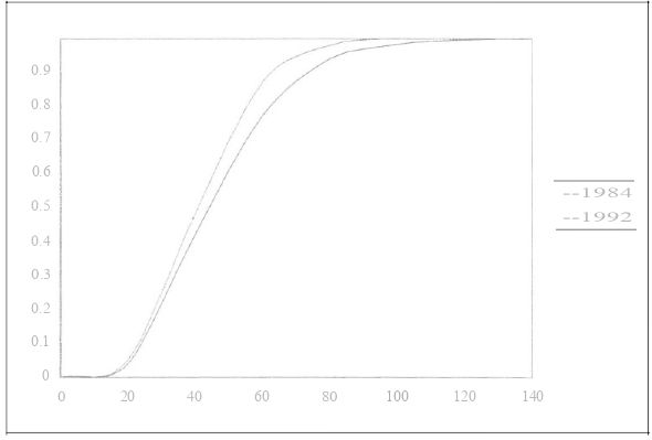
Simulated Distribution Functions of Disposable Income per Equivalent Adult in 1984 and 1992.
Four different simulations have been run on MICROHUS:7
All modules with tax and transfer systems for each year 1984 to 1992. This simulation shows the full set of behavioral (or second and subsequent round) effects from the tax-transfer reform - including full labor supply effects.
As for Simulation 1, but in 1990-1992 no adjustment of annual work hours was permitted- that is, those who were employed in 1989 kept their 1989 hours until 1992. New entries to the labor market and exits caused by retirement or death were, however, permitted. This simulation shows a limited set of behavioral effects from the tax transfer reforms.
As for Simulation 1, but in 1990-1992 no demographic, housing, labor market or income changes were permitted - that is, the tax and transfer systems of 1990-1992 were applied to the income distribution etc. of 1989. In order not to allow inflationary price increases to distort comparisons across years, all wage rate and incomes were inflated by the CPI. This simulation shows the direct or first-round effects of the tax-transfer changes.
As for Simulation 1, but in 1990-1992 the 1989 tax system was used. This simulation thus applies the 1989 tax rules to the 1990-92 world (ignoring the transfer system).
The direct effect of the tax reform is obtained from simulation number 3, by comparing the 1991 and 1992 distributions with the distribution of 1989 from the same simulation. The comparison was based on 1989 rather than on 1990, because marginal tax rates had already started to decrease in 1990 - Table 3 gives the results. The direct effects of the tax reform are an increase in the average level of disposable income and increased income inequality. For instance, applying the 1992 tax and transfer system to the 1989 incomes and taking the difference in price levels into account results in a median real income and a Gini coefficient which are respectively 15 and 12 per cent higher than is the case when the 1989 tax and transfer system is used (Table 3). The increase in inequality is even higher (22 to 32 per cent) among households with children than it is for the whole population. These estimates are higher than those obtained before the tax reform was implemented. A partial explanation is that MICROHUS does not include the benefits which were not liable for taxation before the tax reform but became taxable after the reform. (In addition, it should be noted that in all of these results any differential effects of the increase in indirect taxes are not taken into account.)
Direct Effects of Tax Changes 1990-1992 (Simulation 3)
| 1989 | 1990 | 1991 | 1992 | |
|---|---|---|---|---|
| All households | ||||
| Median disposable income per equivalent adult (1984 SEK) | 41577 | 42852 | 48680 | 47760 |
| Index | 100 | 103 | 117 | 115 |
| Coefficient of variation | 0.325 | 0.342 | 0.383 | 0.364 |
| Index | 100 | 105 | 118 | 112 |
| Gini coefficient | 0.179 | 0.188 | 0.209 | 0.200 |
| Index | 100 | 105 | 117 | 112 |
| Households with children | ||||
| Median disposable income per equivalent adult (1984 SEK) | 36438 | 37299 | 41721 | 41390 |
| Index | 100 | 102 | 114 | 114 |
| Coefficient of variation | 0.247 | 0.272 | 0.325 | 0.311 |
| Index | 100 | 110 | 132 | 126 |
| Gini coefficient | 0.131 | 0.143 | 0.167 | 0.160 |
| Index | 100 | 109 | 127 | 122 |
The behavioral adjustment effects can be estimated by comparing simulations 1 and 2 with simulation 3. Simulation 2 does not permit adjustments in hours of work among those who are in the labor force. A comparison of Simulations 2 and 3 will thus reveal the effects on the income distribution of other behavioral adjustments - for instance, those related to the housing market and to the size and composition of households. A comparison with simulation 1, on the other hand, gives the full behavioral adjustment effect, including all labor supply effects.8
When the 1991 tax and transfer system is applied to 1989 incomes, the model simulates, for all households, a median disposable equivalent annual income of 48,680 kronor (Simulation 3 in Table 4). If behavioral adjustments other than in hours of market work are permitted in 1991, the income level decreases by three per cent (Simulation 2). If a full adjustment is allowed, it decreases by four per cent (Simulation 1). Parallel to this decrease in income level there is an increase in income inequality. When everything else but hours of market work can deviate from their 1989 levels, the Gini coefficient in 1991 increases by seven per cent (Simulation 2). However, when market hours are also allowed to adjust to the new tax system, there is only a five per cent increase in inequality (Simulation 1). A general conclusion is that the behavioral adjustments cause income levels to decrease and inequality to increase. For households with children, the decrease in level is marginally stronger - and the increase in inequality marginally weaker - than for the entire population. The behavioral adjustment effects on inequality for all households amount to about one-third of the direct effects while, for households with children, they are smaller.
Median Disposable Income per Equivalent Adult and Income Inequality in 1991 and 1992 - Comparison of Results for Simulations 1, 2 and 3.
| Measure | 1991 | 1992 | ||||
|---|---|---|---|---|---|---|
| 3 | 2 | 1 | 3 | 2 | 1 | |
| All households | ||||||
| Median disposable income per equivalent adult (1984 SEK) | 48.680 | 47.084 | 46,779 | 47,760 | 45,700 | 44.901 |
| Index | 100 | 97 | 96 | 100 | 96 | 94 |
| Coefficient of variation | 0.383 | 0.419 | 0.406 | 0.364 | 0.408 | 0.391 |
| Index | 100 | 109 | 106 | 100 | 112 | 107 |
| Gini coefficient | 0.209 | 0.224 | 0.220 | 0.200 | 0.215 | 0.207 |
| Index | 100 | 107 | 105 | 100 | 107 | 104 |
| Households with children | ||||||
| Median disposable income per equivalent adult (1984 SEK) | 41,721 | 40.202 | 39,436 | 41,390 | 37,458 | 36,911 |
| Index | 100 | 96 | 95 | 100 | 91 | 89 |
| Coefficient of variation | 0.325 | 0.344 | 0.344 | 0.310 | 0.316 | 0.310 |
| Index | 100 | 106 | 106 | 100 | 102 | 100 |
| Gini coefficient | 0.167 | 0.175 | 0.174 | 0.160 | 0.167 | 0.161 |
| Index | 100 | 105 | 104 | 100 | 104 | 101 |
What type of behavioral changes occurred in response to the tax-transfer changes? In simulation 3 all non-monetary variables are kept at their 1989 values after 1989. Table 5 compares these with the result of Simulation 1, which permits the model to adjust fully to the tax and transfer changes. Panel A shows that the behavioral responses to the tax changes include a small decrease in employment and a corresponding increase in unemployment and retirement. The numbers in the Table are proportions of unemployment, employment etc. in each year, relative to those in 1989 and expressed in index form. As the proportion of unemployed is very small, small changes in this proportion will result in large relative changes.
Behavioral Adjustment Effects 1989 - 1992 (Simulation 1)
| 1989 | 1990 | 1991 | 1992 | |
|---|---|---|---|---|
| A. LABOR FORCE PARTICIPATION ETC. | ||||
| Male adults | ||||
| Unemployed (2 12 months) | 100 | 159 | 218 | 232 |
| Employed | 100 | 100 | 101 | 99 |
| Student | 100 | 98 | 92 | 93 |
| Retired | 100 | 100 | 98 | 106 |
| Other not in labor force | 100 | 96 | 95 | 85 |
| Female adults | ||||
| Unemployed (2 12 months) | 100 | 125 | 187 | 225 |
| Employed | 100 | 100 | 98 | 99 |
| Student | 100 | 99 | 107 | 103 |
| Retired | 100 | 102 | 105 | 103 |
| Other not in labor force | 100 | 96 | 92 | 89 |
| B. ANNUAL HOURS OF WORK | ||||
| Employed males | ||||
| Mean | 100 | 99 | 101 | 100 |
| Coefficient of variation | 100 | 104 | 107 | 151 |
| Employed females | ||||
| Mean | 100 | 98 | 99 | 95 |
| Coefficient of variation | 100 | 108 | 128 | 157 |
| C. HOURLY WAGE RATES | ||||
| Employed males | ||||
| Mean | 100 | 101 | 116 | 107 |
| Coefficient of variation | 100 | 113 | 115 | 116 |
| Employed females | ||||
| Mean | 100 | 100 | 115 | 108 |
| Coefficient of variation | 100 | 144 | 112 | 132 |
Panel B shows that females have decreased their average hours of work after 1989 by a few per cent. This average, however, hides differences in behavior among women. Those who worked short hours shortened their work hours even more and those who worked long hours increased their hours. Panel C shows that (nominal) wages increased for both genders, in particular in 1991 and 1992. Wage dispersion also increased (more for women than for men). The increased inequality in income due to behavioral changes can thus, at least partly, be traced to increased wage dispersion, increased dispersion in work hours among women and, to some extent, to increased unemployment and retirement. Demographic changes and changes in the housing market have a relatively small effect on inequality.9
The behavioral adjustment effect on income inequality should, however, perhaps not be attributed only to the tax reform. The model might have inherent dynamics which could have produced increased inequality independently of the tax reform. This is likely in particular for the sub-model which updates wages. A fourth approach to assess the effects of the income tax reform is to compare the income distributions which would have resulted if the 1989 income tax system had also applied in 1990-1992 (Simulation 4). Thus while the earlier simulations examined the impact of the 1991 tax-transfer system upon either the 1989 or the early 1990s worlds, this simulation tests the impact of the 1989 system upon the early 1990s world. Table 6 shows what changes in work hours, wage rates and income that the model would produce if the 1989 tax system had also applied in 1990-92. Panel B indicates that the inequality of wage rates among males, as measured by the coefficient of variation, increases by 15 per cent from 1989 to 1991 and by 16 per cent from 1989 to 1992. These increases exactly equal the increase shown in Table 5, Panel C.Thus, the conclusion is that the increase in wage rate inequality for males cannot be the result of the tax reform. The same conclusion also holds for women. The rise in wage rate inequality during the early 1990s is thus due to labor market and other changes, rather than to the tax reforms in 1991 and 1992.
Changes in Hours of Work and Disposable Income 1989-1992 if the 1989 Tax System had Applied in 1990-1992 (Simulation 4)
| 1989 | 1990 | 1991 | 1992 | |
|---|---|---|---|---|
| A. ANNUAL HOURS OF WORK | ||||
| Employed males | ||||
| First quartile | 100 | 101 | 103 | 101 |
| Median | 100 | 101 | 102 | 100 |
| Third quartile | 100 | 102 | 103 | 102 |
| Mean | 100 | 102 | 103 | 101 |
| Employed females | ||||
| First quartile | 100 | 102 | 104 | 100 |
| Median | 100 | 100 | 104 | 100 |
| Third quartile | 100 | 102 | 104 | 104 |
| Mean | 100 | 102 | 104 | 101 |
| B. HOURLY WAGE RATES | ||||
| Employed males | ||||
| First quartile | 100 | 88 | 105 | 95 |
| Median | 100 | 97 | 112 | 103 |
| Third quartile | 100 | 101 | 116 | 111 |
| Mean | 100 | 101 | 116 | 107 |
| Coefficent of variation | 100 | 113 | 115 | 116 |
| Gini | 100 | 111 | 115 | 118 |
| Employed females | ||||
| First quartile | 100 | 94 | 114 | 100 |
| Median | 100 | 96 | 115 | 104 |
| Third quartile | 100 | 100 | 118 | 114 |
| Mean | 100 | 100 | 115 | 108 |
| Coetficent of variation | 100 | 143 | 112 | 132 |
| Gini | 100 | 114 | 112 | 120 |
| C. DISPOSABLE INCOME | ||||
| All households | ||||
| First quartile | 100 | 95 | 98 | 96 |
| Median | 100 | 95 | 99 | 97 |
| Third quartile | 100 | 96 | 103 | 97 |
| Mean | 100 | 96 | 101 | 98 |
| Coefficent of variation | 100 | 107 | 108 | 104 |
| Gini | 100 | 103 | 107 | 102 |
| Households with children | ||||
| First quartile | 100 | 96 | 97 | 97 |
| Third quartile | 100 | 97 | 102 | 98 |
| Mean | 100 | 97 | 100 | 97 |
| Coefficent of variation | 100 | 130 | 111 | 101 |
| Gini | 100 | 104 | 111 | 102 |
Panel A of Table 6 shows that work hours would increase by a few per cent if the 1989 tax system had been kept, and panel C shows that the income level would decrease a little and the inequality of disposable income would increase by 2 to 8 per cent.
Table 7 shows the difference between two ‘full behavioral response’ simulations, one using the current tax and transfer systems (Simulation 1) and one imposing the 1989 tax system after 1989 (Simulation 4). For example, the index value of 97 for median employed males’ hours of work in 1990 means that with the 1990 tax system the median was 3 per cent less than with the 1989 tax system. Panel B indicates that the 1991-92 income taxes increased income inequality by 14 to 15 per cent for the whole population and by 20 to 25 per cent for households with children.10 The same panel also shows that the 1991-92 tax system increased the average disposable income level of the whole population by 13 to 16 per cent. Panel A reveals that part of the increased income inequality comes from an increase in the dispersion of work hours for both males and females. In addition, the gender differences in average annual hours of work increased. There were almost no induced changes in labor force participation and there were no additional changes in wage dispersion compared with Table 6.11
An Alternative Assessment of the Total Effects of the 1990-1992 Income Tax Changes - Current Tax System (Simulation 1) Compared to the 1989 Tax System (Simulation 4)
| 1989 | 1990 | 1991 | 1992 | |
|---|---|---|---|---|
| A. ANNUAL HOURS OF WORK | ||||
| Employed males | ||||
| First quartile | 100 | 97 | 97 | 100 |
| Median | 100 | 97 | 98 | 100 |
| Third quartile | 100 | 98 | 99 | 102 |
| Mean | 100 | 97 | 98 | 99 |
| Employed females | ||||
| First quartile | 100 | 94 | 89 | 84 |
| Median | 100 | 96 | 94 | 95 |
| Third quartile | 100 | 98 | 99 | 101 |
| Mean | 100 | 96 | 95 | 94 |
| B. DISPOSABLE INCOME PER ADULT EQUIVALENT | ||||
| All households | ||||
| First quartile | 100 | 101 | 107 | 107 |
| Median | 100 | 101 | 114 | 111 |
| Third quartile | 100 | 101 | 116 | 115 |
| Mean | 100 | 101 | 116 | 113 |
| Coefficent of variation | 100 | 105 | 116 | 115 |
| Gini | 100 | 102 | 115 | 114 |
| C. HOUSEHOLDS WITH CHILDREN | ||||
| First quartile | 100 | 100 | 104 | 102 |
| Median | 100 | 100 | 110 | 106 |
| Third quartile | 100 | 100 | 113 | 112 |
| Mean | 100 | 100 | 111 | 109 |
| Coefficent of variation | 100 | 111 | 125 | 124 |
| Gini | 100 | 102 | 120 | 121 |
5. Conclusions
The simulations with MICROHUS show that the 1990-91 Swedish tax reform increased the inequality of the distribution of disposable income per equivalent adult. The direct effects have been estimated at about 17 per cent in 1991 and 12 per cent in 1992 for the whole population of households. Our initial estimates of the effects of behavioral adjustments (Simulations 1 and 2) suggested about a 5 to 10 per cent additional increase in inequality once behavioral changes were also taken into account. However, most of this effect cannot be attributed to the tax reform but to the dynamic specification of the model which captured, for instance, the rising inequality of wage rates in Sweden in the early 1990s. A second approach to evaluate the effects of the tax reform involved comparing the income distributions obtained with the 1991-1992 tax systems (Simulation 1) with those which would have resulted if the 1989 tax system had still applied in 1991 and 1992 (Simulation 4). According to this comparison, the new tax system generated an increase in inequality of about 15 per cent. When this estimate is compared with the 17 per cent estimate of the direct effects, the indirect behavioral adjustment effect would thus seem to be very small.
The size of the indirect effect will, of course, depend very much on the model specification. In MICROHUS the labor supply adjustments are small, partly because the decision to join the labor force is independent of incentives from the tax system (by assumption) and partly because the estimated wage rate and income elasticities for those already employed are relatively small. The labor supply literature has shown that the participation decision depends more on wage rates and income incentives than does changes in hours of work. A re-specification which introduces more economic incentives into the module, and which simulates entrances to the labor market might thus increase the adjustment effect. The application of supply functions for hours of work of the Hausman type could also be criticized. There is certainly scope for improvements and alternatives. For instance, a good labor supply model should give a better representation of the joint decisions of two spouses.
Although this work has not been able to demonstrate any major indirect, behavioral adjustment effects on the income distribution resulting from the Swedish tax reform of 1991 this might be a consequence of the model specification. It might also take longer than a year or two before these effects become manifest. Additional efforts to design flexible models which predict behavior well are needed before we can be certain that estimates of direct effects alone provide good guides to the total effects.
Footnotes
1.
The model was estimated from the 1984 and 1986 waves of the HUS panel. The log wage rate is thus explained by its lagged value with a lag of two years. The estimated autoregression parameter for females was estimated to be 0.637. The predictions from the model, however, implied an unreasonable decrease in the average female wage rate. For this reason, this parameter was increased to 0.785. The estimate for males was 0.801.
2.
A more detailed description of the treatment of each income component is given in Klevmarken and Olovsson (1994).
3.
For a more detailed analysis of the evolution of the Swedish tax and transfer system in the last few decades see Gustafsson and Klevmarken (1993).
4.
The simulated population size decreases from 5,250 individuals in 1984 to 4,866 in 1992. This is a decrease which has no correspondence in the Swedish population. The explanation is that MICROHUS does not allow for migration.
5.
It should be noted that these comparisons are based on only one single simulation of MICROHUS. Because the model is stochastic, replications of the same simulation will not give exactly the same results. Comparisons with official statistics should ideally be based on several replications. An indication of the built-in stochastic variability of MICROHUS can be obtained from Klevmarken and Olovsson (1994), Appendix B.
6.
The definition oi being unemployed is at least 12 months of unemployment.
7.
All simulations were started with the same seed in order to minimize the influence of random variation when comparing simulations.
8.
This is not altogether true because, in addition to the changes in the tax and transfer systems, the model adapts to exogenous changes in the CPI, the real rate of return on assets, and the average unemployment rate. Of these, the unemployment rate might influence the distribution of income most, but none of these changes are believed to be of great importance for the inequality of disposable income.
9.
For a simulation study of demographic effects on the income distribution see Klevmarken (1994).
10.
Thus the index number 114 for the Gini coefficient in 1992 means that the Gini coefficient from simulation 1 in 1992 exceeded the corresponding Gini coefficient from simulation 4 by 14 per cent.
11.
These results are not shown in Table 7.
APPENDIX A
Simulation 1: Reference Case with Full Model
| A. Age distribution (%) and sample size | |||||||||
| 1984 | 1985 | 1986 | 1987 | 1988 | 1989 | 1990 | 1991 | 1992 | |
| Age | |||||||||
| 0 - 6 | 7.7 | 7.2 | 6.3 | 5.3 | 4.8 | 4.4 | 4.6 | 4.7 | 4.8 |
| 7 - 17 | 14.7 | 14.7 | 15.2 | 15.3 | 15.3 | 14.8 | 14.1 | 13.5 | 12.9 |
| 18-29 | 18.9 | 18.8 | 19.9 | 19.6 | 19.3 | 19.9 | 19.9 | 20.0 | 20.2 |
| 30 - 39 | 15.0 | 15.6 | 15.3 | 14.6 | 15.0 | 14.7 | 14.7 | 14.8 | 15.1 |
| 40 - 49 | 13.8 | 14.1 | 14.6 | 15.3 | 15.8 | 16.4 | 16.8 | 16.9 | 16.9 |
| 50 - 64 | 18.4 | 18.2 | 18.3 | 18.4 | 19.0 | 18.8 | 18.8 | 19.5 | 19.6 |
| 66 - 74 | 11.1 | 11.1 | 11.0 | 11.2 | 10.6 | 10.6 | 10.7 | 10.3 | 10.3 |
| 751 | 0.2 | 0.3 | 0.4 | 0.3 | 0.2 | 0.3 | 0.4 | 0.4 | 0.4 |
| Sample size | 5250 | 5201 | 5170 | 5124 | 5050 | 5011 | 4968 | 4927 | 4866 |
| B. Marital status (%): 18 years and older | |||||||||
| 1984 | 1985 | 1986 | 1987 | 1988 | 1989 | 1990 | 1991 | 1992 | |
| Married | 53 1 | 52.6 | 52.2 | 52.1 | 51.5 | 51.3 | 50.7 | 50.9 | 50.3 |
| Cohabiting | 14.3 | 14.4 | 14.7 | 14.7 | 14.7 | 14.8 | 14.8 | 14.9 | 15.2 |
| Single | 32.6 | 33.0 | 33.1 | 33.2 | 33.8 | 34.0 | 34.5 | 34.2 | 34.5 |
| C. Labor force participation (%); 18 years and older | |||||||||
| 1984 | 1985 | 1986 | 1987 | 1988 | 1989 | 1990 | 1991 | 1992 | |
| Male adults | |||||||||
| Unemployed (≥12 months) | 1.1 | 0.7 | 0.5 | 0.2 | 0.3 | 0.3 | 0.5 | 0.7 | 0.8 |
| Employed | 71.2 | 72.2 | 72.9 | 720 | 71.5 | 68.7 | 68.8 | 69.5 | 68.1 |
| Student | 5.3 | 5.3 | 5.3 | 7.2 | 8.0 | 9.0 | 8.8 | 8.3 | 8.4 |
| Retired | 18.5 | 17.8 | 17.9 | 17.4 | 17.1 | 19.0 | 19.0 | 18.6 | 20.0 |
| Other not in L.F. | 3.9 | 3.8 | 3.4 | 3.2 | 3.1 | 3.0 | 2.9 | 2.9 | 2.6 |
| Female adults | |||||||||
| Unemployed (≥12 months) | 1.3 | 1.8 | 1.2 | 0.5 | 0.2 | 0.4 | 0.5 | 0.8 | 0.9 |
| Employed | 64.1 | 64.5 | 65.4 | 63.6 | 64.1 | 63.3 | 63.3 | 62.1 | 63.0 |
| Student | 5.5 | 5.5 | 5.4 | 7.6 | 8.3 | 8.3 | 8.2 | 8.9 | 8.6 |
| Retired | 18.9 | 18.1 | 18.3 | 19.3 | 18.9 | 19.7 | 20.1 | 20.7 | 20.3 |
| Other not in L.F. | 10.2 | 10.1 | 9.7 | 9.1 | 8.5 | 8.2 | 7.9 | 7.5 | 7.3 |
| D. Annual hours of market work; employed | |||||||||
| 1984 | 1985 | 1986 | 1987 | 1988 | 1989 | 1990 | 1991 | 1992 | |
| Males | |||||||||
| First quartile | 1750 | 1800 | 1764 | 1820 | 1820 | 1800 | 1768 | 1800 | 1813 |
| Median | 1924 | 1950 | 1924 | 1976 | 1976 | 1976 | 1932 | 1960 | 1976 |
| Third quartile | 2080 | 2080 | 2040 | 2132 | 2132 | 2091 | 2080 | 2132 | 2184 |
| Females | |||||||||
| First quartile | 1260 | 1300 | 1274 | 1300 | 1288 | 1300 | 1248 | 1200 | 1092 |
| Median | 1404 | 1440 | 1404 | 1428 | 1421 | 1456 | 1404 | 1428 | 1377 |
| Third quartile | 1551 | 1598 | 1560 | 1581 | 1600 | 1612 | 1612 | 1666 | 1700 |
| E. Hourly wage rates (current SEK); employed | |||||||||
| 1984 | 1985 | 1986 | 1987 | 1988 | 1989 | 1990 | 1991 | 1992 | |
| Males | |||||||||
| First quartile | 38 | 42 | 39 | 41 | 37 | 42 | 37 | 44 | 40 |
| Median | 45 | 52 | 50 | 54 | 51 | 58 | 56 | 65 | 60 |
| Third quartile | 55 | 61 | 62 | 68 | 67 | 75 | 76 | 87 | 83 |
| Mean | 49 | 55 | 54 | 58 | 56 | 61 | 62 | 71 | 65 |
| Coefficent of variation | 0.439 | 0.443 | 0.508 | 0.510 | 0.585 | 0.548 | 0.619 | 0.629 | 0.634 |
| Females | |||||||||
| First quartile | 32 | 37 | 32 | 35 | 33 | 36 | 34 | 41 | 36 |
| Median | 38 | 44 | 41 | 46 | 42 | 48 | 46 | 55 | 50 |
| Third quartile | 46 | 53 | 50 | 57 | 54 | 62 | 62 | 73 | 69 |
| Mean | 40 | 46 | 43 | 48 | 46 | 52 | 52 | 60 | 56 |
| Coefficent of variation | 0.434 | 0.455 | 0.523 | 0.460 | 0.602 | 0.494 | 0.706 | 0.554 | 0.652 |
| F. Household disposable income per equivalent adult (constant 1984 SEK) | |||||||||
| 1984 | 1985 | 1986 | 1987 | 1988 | 1989 | 1990 | 1991 | 1992 | |
| All households | |||||||||
| First quartile | 33792 | 35195 | 33645 | 33840 | 33135 | 33954 | 32602 | 35862 | 34936 |
| Median | 41691 | 44464 | 40475 | 42389 | 39870 | 41577 | 39826 | 46779 | 44901 |
| Third quartile | 51321 | 55475 | 50155 | 52983 | 50272 | 52325 | 50283 | 62945 | 58588 |
| Mean | 43682 | 46681 | 42817 | 44772 | 42645 | 44225 | 42925 | 51649 | 48721 |
| Coefficent of variation | 0.311 | 0.326 | 0.311 | 0.325 | 0.319 | 0.325 | 0.362 | 0.406 | 0.391 |
| Households with children | |||||||||
| First quartile | 32378 | 33803 | 32108 | 32474 | 31676 | 32040 | 30788 | 32545 | 31714 |
| Median | 37903 | 39860 | 36591 | 38173 | 35465 | 36438 | 35139 | 39436 | 36911 |
| Third quartile | 43991 | 47530 | 42879 | 45237 | 42123 | 42909 | 41525 | 49232 | 46780 |
| Mean | 39355 | 41653 | 38308 | 39693 | 37872 | 38190 | 37334 | 42569 | 40448 |
| Coefficent of variation | 0.263 | 0.277 | 0.264 | 0.262 | 0.288 | 0.247 | 0.354 | 0.344 | 0.310 |
-
1
When a household head reaches the age of 75 the whole household is excluded from the sample. Only household members 75 years and older who live in a household with a head younger than 75 remain in the sample.
References
-
1
The Swedish Welfare State in TransitionThe effect of Sweden’s tax and transfer system on labor supply, The Swedish Welfare State in Transition, Chicago University Press.
-
2
En Prognosmodell För Den Allmänna TilläggspensioneringenStockholm: Riksforsakringsverket.
-
3
Welfare and Work Incentives A North European PerspectiveTaxes and transfers in Sweden: Incentive effects on labour supply, Welfare and Work Incentives A North European Perspective, Oxford, Clarendon Press.
- 4
-
5
The impact of demographic changes on the income distribution: Experiments in microsimulationPaper presented to the 8th Annual Conference of the European Society for Population Economics.
-
6
Direct and Behavioural Effects of Income Tax Changes - Simulations with the Swedish Model MICROHUS. Working Paper 1994:20Uppsala: Department of Economics, Uppsala University.
-
7
Hushållens ekonomiska levnadsförhållanden (HUS). Teknisk beskrivning och kodbokDepartment of Economics, Gothenburg University.
-
8
Paper Presented to the International Symposium on Economic ModellingMlCROHUS: A microsimulation model for the Swedish household sector - A progress report, Paper Presented to the International Symposium on Economic Modelling, Gothenburg, Sweden.
-
9
Demographics and the dynamics of earningsJournal of Population Economics 6:105–122.https://doi.org/10.1007/BF00178556
Article and author information
Author details
Funding
No specific funding for this article is reported.
Acknowledgements
This article has been orginally published as Ch. 10 in A. Harding (ed.) Microsimulation and Public Policy, Contributions to economic analysis no 232, Elsevier, Amsterdam 1996.
Publication history
- Version of Record published: April 30, 2022 (version 1)
Copyright
© 2022, Klevmarken and Olovsson
This article is distributed under the terms of the Creative Commons Attribution License, which permits unrestricted use and redistribution provided that the original author and source are credited.