Figures and data in Direct and Behavioral Effects of Income Tax Changes. Simulations with the Swedish Model MICROHUS

Cite this article as: A. Klevmarken, P. Olovsson; 2022; Direct and Behavioral Effects of Income Tax Changes. Simulations with the Swedish Model MICROHUS; International Journal of Microsimulation; 15(1); 135-152. doi: 10.34196/ijm.00257

Article
Figures and data
Jump to

2 figures and 7 tables

Figures

Figure 1

Download asset Open asset

Simulated Swedish Average Marginal Tax Rates by Gender, 1984-1992

Figure 2

Download asset Open asset

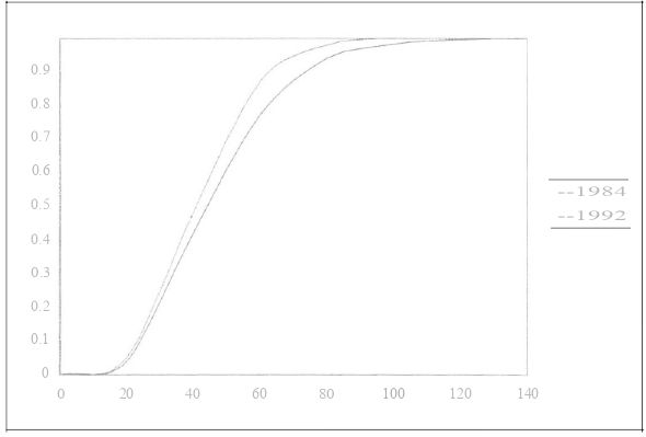
Simulated Distribution Functions of Disposable Income per Equivalent Adult in 1984 and 1992.

Tables

Table 1

Labor Supply Elasticities for Full-time Working Males and Females by Marital Stah1s

	Singles	Couples
	Males and Females	Males	Females
Wage rate	0.143	-0.013	-0.006
Income	-0.581	-0.181	-0.149
Compensated	0.601	0.130	0.112

Table 2

Comparison Between Official Statistics and the Simulations of MICROHUS

	1984	1985	1986	1987	1988	1989	1990	1991	1992
A. LABOR FORCE PARTICIPATION RATES
Males
Labor force survey	85.6	86.0	85.9	85.7	86.2	86.8	87.0	86.0	84.0
Index 1984=1OD	100	100.5	100.3	100.1	100.7	101.4	101.6	100.5	98.0
Simulation 1	72.3	73.0	73.4	72.2	71.8	69.0	69.1	70.2	68.9
Index 1984=1OD	100	101	102	100	99	95	96	97	95
Females
Labor force survey	78.2	79.2	80.D	81.1	81.8	82.2	82.6	81.7	79.9
Index 1984=100	100	101.3	102.3	103.7	104.6	105.1	105.6	104.4	102.2
Simulation 1	65.4	66.3	66.6	64.0	64.3	63.7	63.8	62.9	63.9
Index 1984=100	100	101	102	98	98	97	98	96	98
B. HOURS OF WORK (EMPLOYED)
Males
Labor force survey	40.6	40.7	40.7	41.4	41.4	41.5	41.5	41.2	41.2
(weekly) Index 1984=100	100	100.2	100.2	102.0	102.0	102.2	102.2	101.5	101.5
Simulation 1	1858	1902	1880	1933	1937	1930	1909	1944	1932
(annual means) Index 1984=100	100	102	101	104	104	104	103	105	104
Females
Labor force survey	31.7	32.1	32.3	32.7	33.2	33.5	33.7	33.6	33.5
(weekly) Index 1984=100	100	101.3	101.9	103.2	104.7	105.7	106.3	106.0	105.7
Simulation 1	1391	1443	1418	1430	1445	1451	1429	1440	1376
(annual means) Index 1984=1OD	100	104	102	103	104	104	103	104	99
C. INEQUALITY IN HOUSEHOLD DISPOSABLE INCOME PER ADULT EQUIVALENT (GINI COEFFICIENT)
Statistics Sweden·	0.220	0.221	0.230	0.221	0.221	0.223	0.231	0.261	0.253
Index 1984=1OD	100	100.4	104.5	100.4	100.4	101.4	105.0	118.6	115.0
Simulation 1	0.171	0.181	0.171	0.180	0.173	0.179	0.188	0.220	0.207
Index 1984=100	100	106	100	105	101	105	110	129	121

Sources: Statistiska Meddelanden Be21SM9501, Income distribution survey in 1993 - Statistics Sweden. Labor force survevs, Statistics Sweden.
*

The tax reform in 1991 made various benefits taxable which had previously been exempt from taxation. If these benefits had been taxable in 1990 and included in the income concept the Gini coefficient would have increased from 0.231 to 0.246.

Table 3

Direct Effects of Tax Changes 1990-1992 (Simulation 3)

	1989	1990	1991	1992
All households
Median disposable income per equivalent adult (1984 SEK)	41577	42852	48680	47760
Index	100	103	117	115
Coefficient of variation	0.325	0.342	0.383	0.364
Index	100	105	118	112
Gini coefficient	0.179	0.188	0.209	0.200
Index	100	105	117	112
Households with children
Median disposable income per equivalent adult (1984 SEK)	36438	37299	41721	41390
Index	100	102	114	114
Coefficient of variation	0.247	0.272	0.325	0.311
Index	100	110	132	126
Gini coefficient	0.131	0.143	0.167	0.160
Index	100	109	127	122

Table 4

Median Disposable Income per Equivalent Adult and Income Inequality in 1991 and 1992 - Comparison of Results for Simulations 1, 2 and 3.

Measure	1991			1992
Measure	3	2	1	3	2	1
All households
Median disposable income per equivalent adult (1984 SEK)	48.680	47.084	46,779	47,760	45,700	44.901
Index	100	97	96	100	96	94
Coefficient of variation	0.383	0.419	0.406	0.364	0.408	0.391
Index	100	109	106	100	112	107
Gini coefficient	0.209	0.224	0.220	0.200	0.215	0.207
Index	100	107	105	100	107	104
Households with children
Median disposable income per equivalent adult (1984 SEK)	41,721	40.202	39,436	41,390	37,458	36,911
Index	100	96	95	100	91	89
Coefficient of variation	0.325	0.344	0.344	0.310	0.316	0.310
Index	100	106	106	100	102	100
Gini coefficient	0.167	0.175	0.174	0.160	0.167	0.161
Index	100	105	104	100	104	101

Table 5

Behavioral Adjustment Effects 1989 - 1992 (Simulation 1)

	1989	1990	1991	1992
A. LABOR FORCE PARTICIPATION ETC.
Male adults
Unemployed (2 12 months)	100	159	218	232
Employed	100	100	101	99
Student	100	98	92	93
Retired	100	100	98	106
Other not in labor force	100	96	95	85
Female adults
Unemployed (2 12 months)	100	125	187	225
Employed	100	100	98	99
Student	100	99	107	103
Retired	100	102	105	103
Other not in labor force	100	96	92	89
B. ANNUAL HOURS OF WORK
Employed males
Mean	100	99	101	100
Coefficient of variation	100	104	107	151
Employed females
Mean	100	98	99	95
Coefficient of variation	100	108	128	157
C. HOURLY WAGE RATES
Employed males
Mean	100	101	116	107
Coefficient of variation	100	113	115	116
Employed females
Mean	100	100	115	108
Coefficient of variation	100	144	112	132

Table 6

Changes in Hours of Work and Disposable Income 1989-1992 if the 1989 Tax System had Applied in 1990-1992 (Simulation 4)

	1989	1990	1991	1992
A. ANNUAL HOURS OF WORK
Employed males
First quartile	100	101	103	101
Median	100	101	102	100
Third quartile	100	102	103	102
Mean	100	102	103	101
Employed females
First quartile	100	102	104	100
Median	100	100	104	100
Third quartile	100	102	104	104
Mean	100	102	104	101
B. HOURLY WAGE RATES
Employed males
First quartile	100	88	105	95
Median	100	97	112	103
Third quartile	100	101	116	111
Mean	100	101	116	107
Coefficent of variation	100	113	115	116
Gini	100	111	115	118
Employed females
First quartile	100	94	114	100
Median	100	96	115	104
Third quartile	100	100	118	114
Mean	100	100	115	108
Coetficent of variation	100	143	112	132
Gini	100	114	112	120
C. DISPOSABLE INCOME
All households
First quartile	100	95	98	96
Median	100	95	99	97
Third quartile	100	96	103	97
Mean	100	96	101	98
Coefficent of variation	100	107	108	104
Gini	100	103	107	102
Households with children
First quartile	100	96	97	97
Third quartile	100	97	102	98
Mean	100	97	100	97
Coefficent of variation	100	130	111	101
Gini	100	104	111	102

Table 7

An Alternative Assessment of the Total Effects of the 1990-1992 Income Tax Changes - Current Tax System (Simulation 1) Compared to the 1989 Tax System (Simulation 4)

	1989	1990	1991	1992
A. ANNUAL HOURS OF WORK
Employed males
First quartile	100	97	97	100
Median	100	97	98	100
Third quartile	100	98	99	102
Mean	100	97	98	99
Employed females
First quartile	100	94	89	84
Median	100	96	94	95
Third quartile	100	98	99	101
Mean	100	96	95	94
B. DISPOSABLE INCOME PER ADULT EQUIVALENT
All households
First quartile	100	101	107	107
Median	100	101	114	111
Third quartile	100	101	116	115
Mean	100	101	116	113
Coefficent of variation	100	105	116	115
Gini	100	102	115	114
C. HOUSEHOLDS WITH CHILDREN
First quartile	100	100	104	102
Median	100	100	110	106
Third quartile	100	100	113	112
Mean	100	100	111	109
Coefficent of variation	100	111	125	124
Gini	100	102	120	121

Data and code availability

Please contact the authors for information on data and code availability.

Download links

A two-part list of links to download the article, or parts of the article, in various formats.

Downloads (link to download the article as PDF)

Article PDF

Download citations (links to download the citations from this article in formats compatible with various reference manager tools)

BibTeX
RIS

Open citations (links to open the citations from this article in various online reference manager services)

Mendeley

Simulated Swedish Average Marginal Tax Rates by Gender, 1984-1992

Simulated Distribution Functions of Disposable Income per Equivalent Adult in 1984 and 1992.