Microsimulation for Public Policy. Experiences from the Swedish Model SESIM
- Department of Economics, Sweden
Abstract
This paper reviews policy applications of the Swedish microsimulation model SESIM. These applications include studies of grants and loans to students, redistribution through the public sector and in particular the consequences of population ageing. The paper also discusses the structure and properties of SESIM and demonstrates how the model can be used to evaluate alternative policies.
1. Introduction to microsimulation
Microsimulation models have become common tools for governments to study the distributional consequences of policy changes. For instance, so called tax-benefit models are computer programs that have the tax- and benefit rules of a country coded. This code is then applied to a sample of individuals which has all the information of incomes and other circumstances needed to compute the taxes and benefits that apply to each individual. A tax benefit model thus gives the taxes, benefits and disposable incomes of every individual (household) in the sample. These results can then be used to compute various distributions such as the distribution of disposable income, and the share of poor people in various population subgroups.1 If the purpose of the analysis is to study the consequences of a new policy, for instance a new tax scale, the tax code of the tax-benefit model is changed according to the new scale and the sample of individuals is run through the new code. The results from the new run can be compared to the old in order to evaluate the effect of the new policy compared to the old.
However, a new policy is usually introduced to influence the behavior of people. The tax-benefit model uses the same sample in both runs, i.e., the same income distribution, the same demographic distributions, etc. There is thus no accounting for any adjustments to the new policy. For this reason the tax-benefit model is said to give only the first order effects of the policy change. To include behavioral adjustment people have added behavioral models to the tax-benefit model, for instance a labor supply model. Usually, this model is estimated from cross-sectional data and thought to capture some kind of steady state. The policy experiment is then considered to be a comparison between two steady states – a view which is at least debatable – while there is no information as to the time span needed to reach a steady state.
A different approach is to build a so-called dynamic microsimulation model. It is a model which ages its population endogenously, i.e., it includes demographic models of births, marriages, deaths and possibly also migration – events which may or may not be influenced by policy. Typically, it also includes submodels which capture transitions from one state to another, for instance from schooling to employment, from employment to unemployment, and from employment to retirement, etc. These transitions may directly or indirectly be influenced by changes in policy. A dynamic microsimulation model thus tries to trace out the many different paths people follow through time. To the extent the model is realistic in this respect it is a better tool for policy evaluation than the tax-benefit model with or without behavioral equations, because it tries to mirror what actually happens in the economy through time. There is no need to think in terms of hypothetical steady states. Policy makers are usually interested in what will happen in the next few years or in the upcoming mandate period.
Microsimulation models are primarily designed to analyze distributional issues. One is not only interested in simulating the conditional mean of a distribution but the whole distribution. Typically, microsimulation studies also focus on the properties of specific population subgroups, such as single mothers or those in poverty or unemployment, and study transitions in and out of these states and the properties of people in these states. One of the major advantages of a microsimulation model is that the analyst is not confined to study the average economic man but can build behavioral heterogeneity into the model. On the other hand it is easy to aggregate the simulated output for individuals and households to any desired level of aggregation. Another advantage is that in the model the analyst can use the same policy instruments as the politicians do in real life. There is no need to use, for instance, average tax rates or typical marginal rates, one can instead use the tax schedules, thresholds and eligibility criteria from the tax legislation.
Most of the work on dynamic microsimulation models has been done in the Guy Orcutt tradition, ie one seeks to formulate and estimate models that can reproduce marginal and conditional distributions. Even if these models are based on assumptions of economic optimization by economic agents, they are usually not formulated at the level of single economic agents but try to capture at a more aggregate level the probabilities of certain outcomes. More recently so called agent based models have been developed. They explicitly specify the properties of a number of economic agents and their interaction, for instance a number of job seekers who according to certain rules visit a number of employers to find jobs. This development has primarily taken place in an academic environment, and these models have not yet been used much in practical policy simulations.
The Swedish model SESIM is a model in the Guy Orcutt tradition. Originally it was developed within the Swedish Ministry of Finance for a study of the sustainability of the system for grants and loans to university students. The model has later been developed further and, for instance, used to study the properties of the pension system, life-time redistribution through taxes and benefits, intergenerational redistribution, and the consequences of population ageing.
This paper gives a brief description of the model, and reviews the major applications mentioned above, but with a focus on the application to population ageing. It concludes with a discussion of advantages and short comings of the model.
2. Introduction to SESIM
2.1. Why SESIM was built
The micro simulation model SESIM was first developed in the second half of the 1990s by the Ministry of Finance to evaluate the Swedish system to finance higher education. The main issue was to what extent students were likely to repay the loans the government made available to them. If a person had not repaid all of his/her debt by the age of 65, the remaining debt was remitted. A micro simulation approach was appropriate because it could capture the heterogeneity in student behavior (choice of study program and length of studies) as well as in labor market behavior (choice of job, earnings and interruptions of work).
Later the focus of interest shifted towards evaluation of the new Swedish pension system. Is it as stable financially as the designers of the system claimed, and how high pensions can future pensioners expect? The first issue is primarily one of how population aging, and economic growth will influence the pension system. Using the demographic model, the labor market model and the detailed replication of the pension and tax systems in SESIM it is possible to trace paths of the large baby boom cohorts through the labor market into retirement. Then one can compute the assets and liabilities of the pension system to see if they balance. Economic growth is, however, exogenous to SESIM, but the model can be run with alternative assumed growth trajectories.
In the first years of this century an independent group of academic scientists took the initiative to develop SESIM further to be able to carry out a broader study of the consequences of population aging. Models which simulate health status, utilization of health care and social care were now added. A model which allowed an endogenous choice of retirement age was added too as well as a model for geographical mobility. The model which simulated the distribution of income was also supplemented with a model which simulated the wealth distribution.
2.2. The structure and nature of SESIM
SESIM consists of a model structure translated into a computer program and a data base upon which this program works. The data base is a random sample of about 100 000 individuals drawn from a longitudinal register named LINDA. The design of LINDA is such that the sample for a particular year is a random sample from the Swedish population in the same year. 2 The data base of SESIM applies to 1999. In addition to the data from LINDA it includes a sample of 8000 individuals who are not residents of Sweden but have Swedish pension rights.
The data base of SESIM includes all family members. The definition of family or household in the administrative registers is, however, different from the definition one would like to have for economic analysis. Compared to independent sources LINDA reports too many young adults living with their parents, and too few married/cohabiting couples without common children. For this reason the data base have been adjusted to better agree with these independent sources. (For details see Flood (2008)).
Although the data base is a sample from the Swedish population, we will from now on refer to it as the SESIM population.
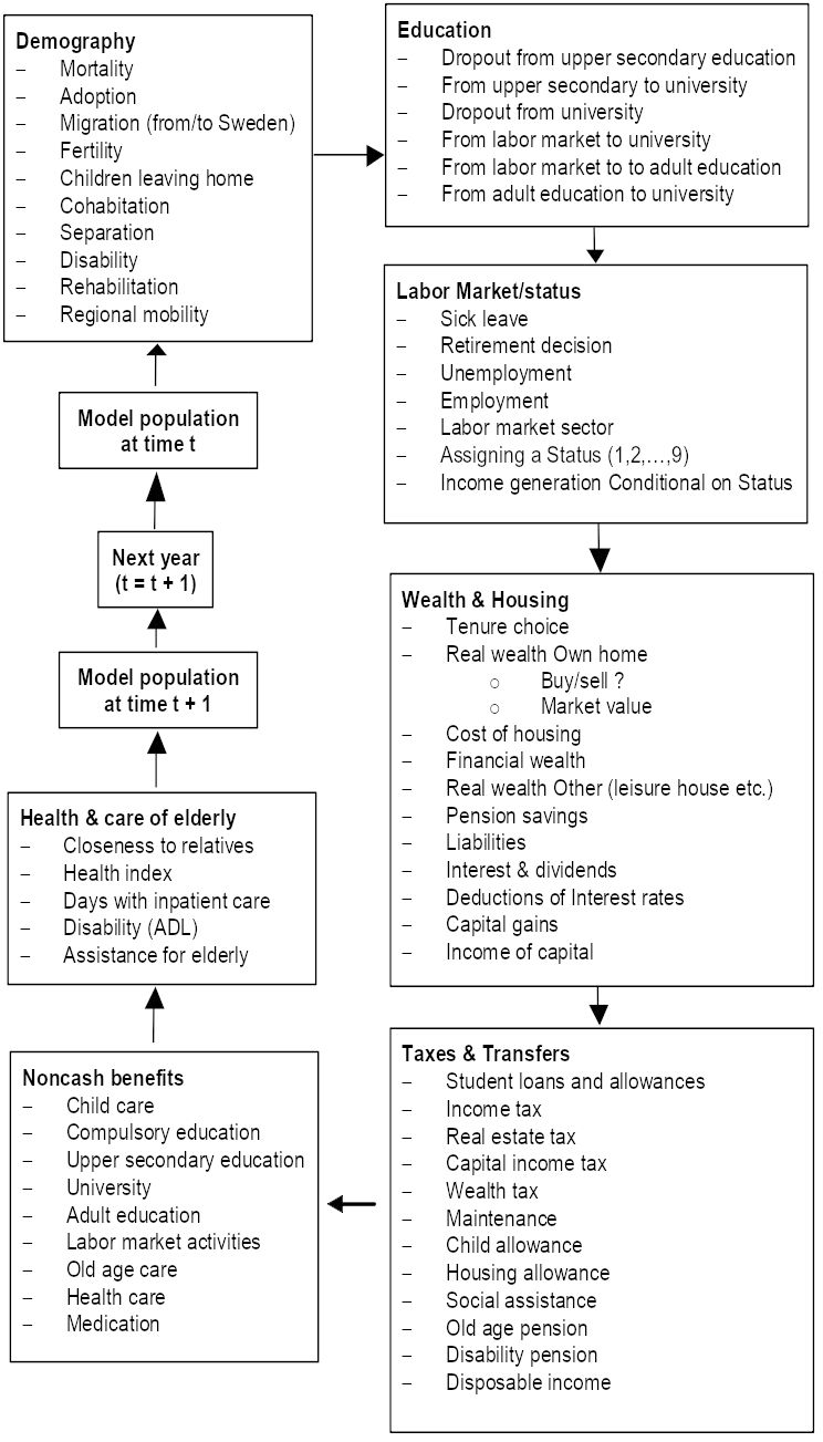
The model structure includes the tax code for personal taxation, the rules that govern benefits and transfer payments to the household sector, in particular social security pensions, and also the rules for the most important occupational pensions. SESIM also includes a number of behavioral models such as forming a union, giving birth to a child, choosing education, taking a job, retiring, etc. The model structure of SESIM is best illustrated by Figure 1.

Structure of SESIM (Source Flood (2008a)). Note: The module “Noncash benfits” was not used in the project on population ageing, it was instead replaced by the module “Health and care of elderly”.
Each box in the diagram includes a number of activities and submodels which rule these activities. All submodels within a box are called a module. Simulations are done sequentially in the order indicated in the diagram. Data are annual data and the time unit of SESIM is a year. SESIM thus starts with the base year data of 1999. Each individual in the SESIM population runs through all the boxes in the diagram starting with the demographic box. First a death probability is computed, and if a uniform random number on the interval (0,1) does not exceed the computed probability, the individual dies. Then the simulation stops for this individual. If however, the individual is simulated to live he/she continues to the submodels for adoption, migration, etc until all demographic models have been passed. The next individual then runs though the same loop until all individuals have run through the demographic module. The simulation then continues module by module until the models for health status, health care and social care have been passed by all individuals. The SESIM population has then become updated for one year, both in the sense that some people have died, children have been born, some have emigrated and some have immigrated, and in the sense that the properties of people have changed, ie they might have added a year of education, got a new job, increased their earnings, moved to another municipality, bought a house, etc. SESIM is thus a dynamic microsimulation model in the sense that the population is aged endogenously. It does not necessarily mean that the behavioral relations used are dynamic in the sense that they use information from a past year. Some of them are, but not all.
There is in general no interaction or stochastic dependence between different individuals with the exception of household members. In some models, for instance the models that determine the wealth distribution, and the models for geographical mobility and tenure choice, the decision unit is the household. There are also models that use “neighborhood” variables, such as the regional unemployment rate in the model that simulates regional moves, and the municipal tax rate in the module that computes taxes and disposable income.
The behavioral models do not have a uniform functional form, but we have chosen the model that fitted best to explain behavior and to simulate, given data available. There are thus a number of different types of models within SESIM. Common choices are probit and logit models, selection models and so-called two-part models. For instance, access to disability insurance is determined by a logit model, which gives the probability to get a disability pension as a function of health status and socio-demographic properties of the individual. (To become disabled is not seen as a choice subject to economic incentives.) Each individual who is simulated to get a disability pension then gets it according to the rules in the social security legislation, usually a percentage of past labor incomes.
For a description of functional form, explaining variables and population at risk for each behavioral model see Flood (2008). A more detailed discussion of choice of model structure, estimation and estimation results for the more recently developed models is found in Klevmarken and Lindgren (2008).
The behavioral models have been tested and estimated using conventional econometric methods. Whenever possible LINDA has been the data source used, not only the 1999 cross-section but the entire longitudinal data set. It is a great advantage to use the same data source for estimation and simulation. It avoids problems of inconsistent definitions of units and variables. However, the administrative data of LINDA have not always allowed us to estimate the models we needed. We then had to use alternative data sources - survey data and register data. Even if these data made it possible to estimate reasonable models, our modeling choices were still constrained by SESIM and LINDA, because if SESIM was unable to simulate all explanatory variables of a model, it could not be used in SESIM. For instance, there are no health data in LINDA and we needed to simulate health status as an input to explain sickness, retirement and utilization of health care and social care. A model for health status was thus estimated from combined survey and register data. This was a dynamic ordered probit model. The probability for a certain health status depended on past status and a number of socio-economic variables. To simulate this model we would in principle need observed data on health status in the base year 1999, which we did not have. The solution was to simulate a reduced model – an ordered probit model, which only depended on the observed socio-economic variables, and use it to impute health status for all individuals in 1999. The same model was also used for people who entered the SESIM population during the simulation.
The sequential structure of SESIM implies that the outcome of an event that lies early in the sequence can influence the outcome of an event that comes later, but not vice versa. A late event can only influence an early event with a lag of one year. This is a practical arrangement from a simulation point of view, but not necessarily a realistic representation of reality. For instance, market work and earnings might be jointly determined, and decisions to move to another municipality might also be joint with decisions about job and housing. Furthermore, the event sequence of Figure 1 does not necessarily represent the time sequence of decisions in a year. The time sequence might be different for different individuals and not necessarily the same in one year as in another year.
Most microsimulation models start with the basic demographic events such as marriage, birth of a child, separation and death, because the outcomes of these events are thought to shape much of the behavior of household members. Schooling will also determine much of post school behavior, and it is thus reasonable to have the education module early in the sequence. Labor market work and earnings will determine consumption and savings and should for this reason precede these two activities. Taxes and benefits cannot be computed until the incomes of a household have been determined. The health module is now the last module in SESIM. Alternatively, we could have placed the health status model before or after the education module, while health care and social care are public benefits in Sweden and thus naturally comes at the end of the sequence jointly with other benefits. If we had started to build SESIM from scratch we had probably chosen to place the health status model early, but now the health module was added to an already existing simulation model, and we did not want to break up its structure and reprogram.
One might also note that the sequential structure of the model in general have implications for the estimation of the stochastic behavioral models of SESIM. If these relations are stochastically uncorrelated each relation can be estimated separately, while if relations are stochastically dependent, they should be estimated jointly. (Cf. the old discussion of recursive and interdependent models.)
A particular feature of SESIM is that each individual each year is assigned a “status”. There are nine different statuses, and with the exception of the status emigrated an individual can have one and only one status in a year. The nine statuses are:
child (0-15 years old)
old age retired; individuals with income from old age pension
student; individuals who study at gymnasium, adult education or university
disabled; individuals who have disability/sickness benefits
parental leave; women who give birth during the year
unemployed; individuals with income from unemployment insurance or from labor market training
miscellaneous
employed; individuals in market work
emigrated; individuals living abroad with Swedish pensions rights. (Note, this classification is not unique because emigrated can have income from early or old age pensions.)
Status determines income: For employed (status 8) earnings are determined by an earnings function, unemployed (status 6) get unemployment compensation according to the rules for this kind of benefits, disabled (status 4) get disability pension, etc. The assumption that one can only have one status in a year is of course not fully realistic. In real life one can for instance, both study and have a job in the same year, and it is also possible to be retired in the sense of drawing a pension and at the same time do market work. In our study of population aging (c f section 3.5 below) the mechanisms through which people leave the labor market was important, and not being able to allow for part-time work and part-time retirement was an unfortunate constraint. However, the decision about the status concept was taken early in the construction of SESIM and it is a key concept in determining the direction of simulations. To drop the status concept or to give it a different meaning had implied that we had to reprogram the model completely.
SESIM is a stochastic simulation model, which means that all events that involve a behavioral model are the result of a stochastic experiment, a draw of random numbers. The outcome of one simulation round will therefore in general differ from the outcome of another one, even if the starting point was the same. This is not only the result of drawing different random numbers but also of the model choosing different paths as a result of different outcomes of the random experiments. For instance, in one simulation an individual might have been simulated to participate in market work, while in another he might have become unemployed. As unemployed he will get lower income, which will have implications for other choices.
One way to reduce the random variation created by the stochastic properties of the model is to increase the sample size, another to use methods that are based on replicated simulations such as the bootstrap method, and a third approach is to align the model to known totals or means, ie the model is forced to replicate these totals and means.3 In SESIM alignment is usually used in the demographic module to make simulated population totals such as the age specific number of births, number of deaths and number of migrants coincide with the demographic statistics and forecasts from Statistics Sweden. It is also used to make the total number of unemployed agree with official statistics and the medium-term forecasts of the Ministry of Finance.
Another reason to align to official forecasts like the demographic forecasts of Statistics Sweden is to make the outcome of the simulations comparable to other studies. One avoids in this way that differences in demographic scenarios explain differences in other target variables, such as for instance the number of elderly that utilize social care.
Alignment can, however, be misused. If the model systematically simulates totals which differ significantly from known totals, it suggests that the model is misspecified or that the parameter estimates are erroneous. The correct action is then to re-specify and re-estimate the model, not to force it on track by alignment. Even if alignment will make the model replicate the known totals there is no guarantee that the distributions around the means implied by the totals will become correct, and these errors will tend to spread to other modules as the simulation proceed.4
SESIM is limited to the household sector and there is no macroeconomic feedback built into the model. Instead it is possible to feed certain macro indicators exogenously into the model. They are: the annual rate of inflation, the rate of return to bonds, stocks and shares, the annual average rate of change in wage rates, and the unemployment rate. It is thus possible to simulate under alternative growth and business cycle scenarios, but there are no market price changes resulting from the actions of households.
3. Policy applications of SESIM
3.1. Public support to students
3.1.1. Policy issues
Higher education in Sweden is free of admission charges and the government also provides loans and cash benefits to students. The sum of loans and benefits should in principle cover student housing, food, insurances and study material during forty weeks of a year, but in practice the cost of living for an average student has from time to time exceeded the support provided by the government. The cash benefit is about one third of the total, while two thirds is a loan.5 Before 2001 a student did not have to start repaying the loan until he/she had a job and labor incomes. Then 4 per cent of the tax assessed income was deducted as interest and payment towards the principal. If the loan was not fully repaid at the age of 65, it was remitted. 6
An issue of policy interest was thus to predict the share of students that would never fully repay their loans and the total cost to the government of this remittance. The first version of SESIM was used for this purpose. The study, Ericson and Hussénius (2000), utilized the potential of SESIM to simulate the whole life-cycle and compute life-cycle incomes net of taxes and the charges for the study loans. In cross-sectional studies grants to students who have no or only low incomes are typically shown to equalize the distribution of income, but in a life-cycle perspective this result is not that obvious. A second objective of the study was thus to evaluate how the life-cycle return to education depended on the length of studies and on gender.
3.1.2. Simulation results
Assuming that the conditions at the end of the 1990s prevail in the future, the model was simulated until it reached a steady state in which the number of births equaled the number of deaths and the population shares in each status were constant. Then people were followed until they died. In this way the results were not influenced by population changes and fluctuations in the supply of higher education. The simulations were also done using the assumption of no growth. The reason was that in a growing economy tax scales and benefits will have to be adjusted, and in the absence of rules for automatic adjustments one would have to predict what politicians would do in a distant future. To avoid this problem no growth was assumed.
Total income was defined in the following way: The sum of labor incomes, pensions, incomes of capital, study loans and cash benefits to students, less the sum of income tax, tax on capital incomes, repayments towards the principal of study loans, and interest on these loans. Labor income included earnings, sickness benefits, parental benefits and unemployment compensation. Pensions included old-age pensions and disability pensions, but not occupational pensions.7
Life-cycle income is the sum of all total incomes from the age of 16 until the person dies. They were only computed for those who were simulated to reach the age of 60. Table 1 gives life-cycle incomes by length of schooling and by gender using the assumption that the interest rate on study loans was 1.3 per cent. We find that males have higher life-cycle incomes than females and that more schooling increases life-cycle income. The excess rate of return to university training relative to no university is higher for females than for males. The explanation is that the difference in length of working life between those with a university degree and those without is higher for women than for men. Women also live longer and thus enjoy the pension benefits for a longer period.
Life-cycle incomes and return to higher education.
| Non university program | Short university program | Long university program | ||||
|---|---|---|---|---|---|---|
| Males | Females | Males | Females | Males | Females | |
| Life-cycle income (1000 SEK) | 6974 | 5120 | 7727 | 5911 | 8861 | 6752 |
| Total return to education (1000 SEK) | 0 | 0 | 753 | 790 | 887 | 631 |
| Rate of return to education per year % | 6.0 | 8.7 | 4.9 | 6.3 | ||
-
Source: Table 5.2, Ericson and Hussénius, 2000.
Table 2 displays how the share of students with loans who get their loans remitted at the age of 65 depend on interest rate, gender and length of schooling. The results are quite sensitive to the assumption about interest rates. Females have much higher remittance rates than men. The explanation is that they work less in the market and get lower incomes. The rate also increases with the duration of the studies because the loans then increase in size and the time span with market work becomes shorter.
Share of students with loans who get their loans remitted at the age of 65 by gender and length of schooling.
| Interest rate (%) | |||
|---|---|---|---|
| 0 | 1.3 | 2.8 | |
| Males | 7.6 | 21.7 | 38.2 |
| Females | 26.1 | 41.4 | 53.2 |
| Less than university | 5.0 | 7.4 | 13.2 |
| Short university | 4.4 | 11.1 | 17.7 |
| Long university | 23.3 | 41.8 | 58.8 |
-
Source: Tables 5.7 and 5.8 in Ericson and Hussénius, 2000.
Even with moderately high interest rates these shares are pretty high and the total amount remitted is of about the same size as the total of all cash benefits. The government decided already in 2001 to make the rules governing repayments less generous, such that almost all students would have to repay their loans completely before the age of 65.
3.2. Lifetime Redistribution through taxes, transfers and non-cash benefits
3.2.1. Policy issues
Which are the redistributive effects of taxes, transfers and non-cash benefits? To what extent do these effects depend on the length of the perspective – a year or a life-cycle?
To what extent does the redistribution performed by the public sector reallocate resources between individuals, and to what extent does it result in an intrapersonal redistribution, for instance from working life to old age?
These issues were studied using the capability of SESIM to simulate whole life-cycles. The results can be found in SOU 2003:110 (2003); SOU 2004:11 (2004) and in Pettersson and Pettersson (2007). The authors claim that a life-cycle perspective is indispensable when designing new taxes and benefits. If it is forgotten in favor of only a short-term perspective, one will not see that the long-run effects of a new policy might not become those intended.
3.2.2. Simulation results
Total income was defined as disposable income less indirect tax paid divided by an equivalence scale, plus non-cash benefits without equivalence scale adjustment. Life-cycle income was then defined as the mean of all total incomes over the life-cycle.
Table 3 displays how the Gini coefficient depends on income concept. Life-cycle incomes are more equally distributed than annual incomes, and total income is more equally distributed than disposable income, which in turn has a Gini coefficient that is about half of that of market incomes. Taxes and benefits thus have a major equalizing impact on the income distribution.
Gini coefficients by income concepts.
| Annual income | Life-cycle income | |
|---|---|---|
| Market income | 0.490 | 0.196 |
| Equivalent disposable income | 0.217 | 0.102 |
| - Indirect taxes | 0.224 | 0.104 |
| + Non-cash benefits | 0.189 | 0.086 |
-
Source: Table 1, Pettersson and Pettersson (2007).
The authors also decompose the Gini coefficient into a weighted sum of concentration indices to investigate how the various income sources contribute to the total Gini. They find that most income sources, such as social security, transfers to family and children, student benefits and income taxes are progressive both annually and in the life-cycle. Market income, occupational pensions, expenditures for old-age care and indirect taxes are regressive.
The only major income source which shifts from progressive to regressive when one goes from annual incomes to life-cycle incomes is old-age pension. In a cross-section of annual incomes old-age pensioners usually have lower incomes than average, but in a life-cycle perspective high pensions are based on high incomes, and high-income earners also tend to live longer than average.
Even if almost all income sources have the same type of impact on the Gini coefficient for annual as well as life-cycle incomes, the relative contribution to the Gini depends on time horizon. For instance, the regressive effect of market incomes is less on life-cycle incomes than on annual incomes, while the regressive effects of disability pensions and income taxes are higher on life-cycle incomes than on annual incomes.
This study also analyzed who is gaining and who is losing over the life-cycle by the public sector. Those who get more transfers and non-cash benefits than taxes paid will have a net gain. In this part of their study the authors did not only include direct taxes but also indirect taxes and social security contributions to the extent that the sum of all taxes paid equaled all benefits received for each cohort. They thus assumed each cohort to be financially balanced over the life-cycle. Furthermore, all economic resources of a household were divided equally among all household members, ie no equivalence scale was used. Table 4 summarizes some of the findings.
Gains and losses through the public sector by gender and income quintile (1000 SEK in 2003 price level).
| Men | Women | Quintiles of Life-cycle income | All | |||||
|---|---|---|---|---|---|---|---|---|
| Q1 | Q2 | Q3 | Q4 | Q5 | ||||
| Taxes | 7136 | 6389 | 4264 | 5741 | 6597 | 7691 | 9483 | 6758 |
| Transfers | 3562 | 4085 | 3924 | 3983 | 3915 | 3770 | 3543 | 3827 |
| Non-cash benefits | 2611 | 3245 | 2840 | 3109 | 3109 | 2922 | 2679 | 2932 |
| Net effect | -963 | 941 | 2500 | 1351 | 428 | -999 | -3262 | 0 |
-
Source: Tables 4 and 5, Pettersson and Pettersson (2007).
There is redistribution from men to women. Women have lower incomes and thus pay less in taxes. They receive more benefits such as maternity and family benefits, and at least partly because they live longer, they get more health care and social care.
There is also a clear redistribution from high to low-income households. The latter pay much less in tax and receive more in transfer payments, while non-cash benefits are more evenly distributed.
There are clear age profiles in the payments between the households and the public sector. Taxes are predominantly paid in working age while benefits are received in the beginning and in the end of the life cycle. Child and family benefits and education come early while old-age pension and health and social care come at the end of life. The balance of payments from and to the public sector starts to become positive at the age of 55, but the cumulative net payments do not become positive until the age of 87. There is thus redistribution from individuals with a short life to those who live long.
Finally, the authors also investigated to what extent redistribution through the public sector resulted in transfers of resources between individuals. They found that only about 18 per cent of the total redistributed was truly a reallocation between individuals, while 45 per cent was annual intra-personal reallocation (benefits in a year were self-financed through own taxes in the same year) and 38 per cent life-cycle intrapersonal reallocation (old-age benefits were self-financed by taxes paid earlier in the life-cycle).
3.3. Intergenerational redistribution
3.3.1. Policy issues
Almost 50 per cent of total production in Sweden is redistributed annually through the public sector. This is done by taxes and fees that are returned to the population in the form of benefits, transfer payments and public consumption. As we have just seen most of the annual redistribution is returned to the same individual – immediately or later in life, for instance as pensions – while a smaller share is redistributed between individuals.
Much of this redistribution builds on an implicit contract between generations. The working population pays taxes and fees to finance childcare, schooling, pensions, health care and old age care - services which are primarily consumed by younger and older people - hoping that their children will do the same when they grow into working age. When the size of birth cohorts varies the issue of redistribution between generations arises. For instance, the large post World War II baby boom cohorts had to put up with large school classes and a fierce competition to enter into universities. Their benefits per capita were thus reduced. These cohorts are now retiring and wondering if they will get the generous pensions they have been expecting. In another 10-15 years they will get to the age when they will need much more health care and social care. Will the government be able to continue providing these services? The children of the baby boomers, cohorts which are smaller in size, might ask if they have to pay for the increased provision of public services to their parents by much increased taxes.
To address these issues a study was started within the Ministry of Finance (Pettersson et al., 2006) with the task to assess the size of any redistribution between now living generations. They also tried to estimate the total life-time consumption potential of a birth cohort, defined as life-time income adjusted by any transfer to or from other generations through the public sector.
3.3.2. Methodology and results
The idea was to compute a life-cycle balance account for each individual of all payments from the individual to the public sector and all payments from the public and services provided by the public sector. These balances were then summed for each birth cohort. An obvious problem is that we do not have observable data covering the whole life-cycle of an individual. The solution was to use the pieces of data that existed and supplement with simulations from the SESIM model. The cohorts studied were born in 1930-2009.
Individual longitudinal register data exist from 1968, but more completely from 1987. Transactions before then were imputed using the latest know distribution and totals from the national accounts as well as various other sources. All transactions after 2004 were simulated by SESIM.
The motivation for this micro(simulation) approach was the following:
Even if a cohort had a positive (negative) balance, all cohort members might not have it. There might have been some groups within the cohort which had been in advantage (disadvantage) while others had not. With a microsimulation approach one can analyze the distribution within cohorts.
The precision in the simulations of future taxes and transfers becomes much better in a microsimulation approach compared to a more aggregate one, because most tax and benefit systems are non-linear.
The microsimulation approach permits the analyst to quite flexibly study the balances for other subgroups than birth cohorts, which makes it easier to understand the outcome and make error corrections.
There are a number of fundamental problems the analysts had to address, and the reader is referred to their report for a discussion. Here I will only briefly mention a few. First, all transactions with the public sector, whether they are with the business sector or a foreign agency, are in the end considered to benefit the private consumer. For instance, expenditures for the defense, roads, etc are allocated as benefits across all individuals. Likewise, all incomes of the public sector are debited to the household sector.
Second, some kind of discounting is needed to make balances from different years comparable. It is relatively easy to index by a consumer price index8 , but one might also like to correct for the real growth of the economy. This becomes especially clear when one compares consumption potentials.9 The authors have chosen to discount with an index of GDP per capita in current prices.
Third, some incomes (and benefits) are individual while others are given to the household. In this study the authors have chosen to assume that there is redistribution within the family such that all family members including children live on the same standard. All incomes are thus allocated equally to all household members and likewise for public consumption. If, for instance, a child goes to a public daycare center at a cost for the taxpayers of say 100 000 SEK per year, these 100 000 are split equally between all family members.
SESIM only simulates the household sector incomes, taxes and transfer payments. The share of the public sector not covered by SESIM was simulated using a macro model called FIMO, and the result was distributed to the individuals in the household sector. It is a model based on the national accounts which simulates annual public incomes and expenditures at a rather detailed level for the government, local governments and the pension system. It also includes the most important macro-economic variables such as GDP, the labor force, prices, interest rates etc. and the population by gender and age groups. The core of FIMO is an aggregate representation of the rules for taxes and transfers. The model does not allow the population to adjust endogenously to changes in taxes and benefits, but such changes have to be imposed on the model exogenously. SESIM and FIMO were run in parallel using the same exogenous assumptions about population changes, productivity, prices and interest rates. For instance, the real wage rate was assumed to increase by 2 per cent annually, the labor force participation rate was set to 80 per cent in the age bracket 16-64, consumer prices were assumed to increase by 2 per cent annually and the interest rate on financial assets was 3 per cent. The sum of all individual taxes and transfer payments simulated in SESIM did not always agree exactly with the corresponding items in the national accounts and in FIMO. The difference was then distributed equally across all adults.
All simulations assumed unchanged policy, ie the tax system and the rules for transfer payments that applied in the beginning of the current century were assumed to remain unchanged. However, some transfers are not indexed, and some are only indexed by the CPI. In order not to decrease the welfare state all transfers and benefits were indexed by the annual average change in wage rates.
The simulations also assumed that the public finances were stable throughout the entire simulation period, ie the public debt as a share of GDP should be about the same at the end of the simulation period as at the beginning. The budget target of a surplus of 2 per cent over a business cycle was also enforced. Real welfare expenditures per capita were assumed unchanged while the effects of the demographic changes were allowed to go through fully. The budget target was maintained through the tax changes.
The welfare state has grown and the expenditures for transfer payments and for public consumption have increased. To finance the growth of the welfare state taxes have increased from about 10 per cent of GDP in the 1930s to about 50 per cent in the 1980s. After that and in the simulated future the GDP shares of taxes, transfers and public consumption stay approximately constant.
Both transfer payments and public consumption primarily benefit the elderly. The public pension system has expanded and become more generous and health care and old age care has also increased. Most of the tax burden is, however, carried by the working population, in particular those in the age bracket 40-65.
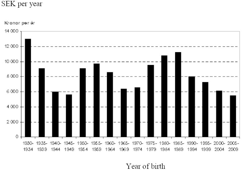
Figure 2 displays the public sector balances by birth cohort. One might have expected some to be negative and some positive, but they are all positive. The explanation is that the public debt was assumed to be a constant share of GDP, and in combination with economic growth increasing debt makes this result possible. We should thus compare the relative size of these bars. The generations with a relative gain are those born in the 1930s, 1950s and 1980s, while the large baby boom cohorts of the 1940s and 1960s are relative losers. Those born in the 1930s paid relatively low taxes but were able to get the benefits of the increasing welfare state. Those born in the 1980s paid relatively little in tax because they started to work late and were assumed to retire early and use their increased longevity for leisure. The generations of the 1950s paid marginally more in taxes compared to those born in the 1940s but got more both in transfer payments and public consumption. The baby boom cohorts of the 1940 worked a rather long life and thus paid relatively much in tax, while they had to compete for the benefits from the public sector.

Public sector balances for people born in 1930-2009. (SEK, average per year of survival in Sweden adjusted for price changes and real growth.)
The results suggest that the increased pressure on the public sector from the large cohorts has not been met by increased taxes but rather by a reduction in the benefits. The same is true for the children of the baby boom cohorts, those born in the 1960s. The youngest cohorts are also losers in these computations. The explanation is that they pay relatively high taxes but get less of future pension benefits. They were assumed to retire at the age of 65, and if the retirement age does not increase with increasing longevity the current pension system will pay out lower pensions.
Within all generations there are individuals who gain from the public sector and others who loose. In fact, this intra generation redistribution is much larger than the inter generation redistribution.
This study also shows that the average consumption potential by cohort – adjusted for price changes and growth – is completely dominated by the market incomes, while the modest intergenerational transfers through the public sector means relatively little. The results suggest that those who were born in the late 1930s and in the 1940s had a little higher consumption potential than the other generations. The explanation is that these generations came out from the schools into a labor market with a high demand for labor and very little unemployment. They got well paid jobs, were able to save and borrow to buy a home, which then increased in value. Although the baby boomers might have lost in the redistribution game through the public sector they were not losers in a wider perspective.
3.3.3. Conclusions
Most of the taxes an individual pays in a life-time go back to the same individual in the form of transfer payments and public consumption. Only about 20 per cent of the taxes an average individual pays result in redistribution to someone else, and most of this redistribution goes to someone in the same generation rather than to someone in another generation.
This study is limited to redistribution through the public sector and does not include private transfers such as inheritance and inter vivo gifts. Nor does it include indirect behavioral effects of public policy, for instance, increased public expenditures on schooling, which increases the educational standard of the population, might lead to different decisions as to work, incomes and wealth accumulation. The informal sector is not included either. In the older generations it was common among women to work at home. Not including this kind of informal work underestimates the consumption potential for the older generations.
Simulating the future with SESIM and FIMO made it possible to fill in the gaps of missing data. Because both models could be calibrated to the same demographic scenario and used the same macro-economic assumptions, it was possible to run the two models in parallel. A closer integration of the two models might have opened for a more realistic distribution of public consumption than equal distribution to everyone.
The results obtained also depend on assumptions about the costs for health care and public care and in particular on the assumption that everyone retires at 65. The increase in the costs of health care and social care is difficult to predict, because they depend on the introduction of new drugs and new treatments and on the ability of the care organizations to increase productivity. New drugs and new treatments are often expensive, but they might increase productivity.
The assumption that everyone, who retires with old-age pension, does it at the age of 65 is unrealistic. The share of people who retire early is not small. It would have been interesting to allow people to retire both before and after 65 in the simulations. SESIM now includes a model with this facility (c f section 3.5). If the incentives of the new pension system and the current policy to give large tax rebates to those who work after the age of 65 make the younger generations stay longer in the labor market, the redistribution between generations would have come out differently.
3.4. The pension system
The Swedish pension system went through a major reform in the early 1990s. The old pay-as-you-go pensions based on the incomes during the fifteen best years were replaced by pensions determined by all work incomes from entry into the labor market to retirement. These pensions are thus of the type of defined contributions, but a large share is still pay-as-you-go pensions, while only a small share is funded. The new system also introduced incentives to postpone retirement and a mechanism to reduce pensions if the liabilities exceeded the funds and the expected future inflow to the system – the so called “brake”.
3.4.1. Policy issues
After the introduction of the new pension system research and policy interest has focused on the behavior of the system, in particular when the large baby boom cohorts retire and age. Interesting issues were: What share of GDP will the pension expenditures take? Will the system stay in financial balance, or will the brake reduce pensions? Which compensation rates will the retired get, and will the inequality of pension incomes increase?
3.4.2. Simulation results
SESIM has been used to simulate the future path of the pension system. This has been done for the European Union Ageing Working Group (see for instance Sundberg, 2006), the medium-term planning of the Ministry of Finance (SOU 2004:11, 2004, p. 11), in preparing for a new administration of the pension system (SOU 2006:111, 2006, p. 111) and by independent scholars (se for instance Flood, 2007 and Section 3.5 below).
The results show that the expenditures for public pensions will take an increasing part of GDP as the baby boom cohorts retire and will reach a maximum of almost 15 per cent around year 2040 (Diagram 6.2 in Sundberg, 2006). With the assumptions made the pension system will generate a surplus every year until 2050, although a declining one, and the financial assets of the system will thus increase. According to these simulations it would not become necessary to hit the brake. However, these simulations are now history, because the current financial and economic crisis has changed the scenario completely and the brake will become enforced already in 2010.
The simulations also show that the compensation rate will decrease for the younger generations unless they chose to retire later. With increasing longevity, the notional pension capital will have to cover a longer period and the annual pensions will then have to decrease.
Flood (2007) demonstrates that variations in retirement age and return on financial assets are more important for the young cohorts than for the old. He computed replacement rates for disposable income10 and showed that for people born in 1940 and with incomes in the middle of the income distribution, the replacement rate at the age of 68-72 was 73 per cent if they retired at the age of 63, but 81 per cent if retired at 67 – a difference of 8 percentage units. For people in the same income class but born in1960, the replacement rates were 56 and 66 respectively – a difference of 10 percentage units.
If the retirement age was 65 but the annual return to financial assets was either 3 per cent or 7 per cent, the replacement rates for those born in 1940 were 73 per cent and 76 per cent respectively – a difference of 3 percentage units. For the cohort of 1960 the replacement rates became 55 and 73 percent respectively – a difference of 18 percentage units!
The explanation to the differences between the two cohorts is that the 1940 cohort mainly gets its pensions according to the old system and time has not permitted them to accumulate large funds in the funded part of the new system.
3.4.3. Conclusions
The focus in SESIM on demography, income generation, taxes and pensions makes it a good tool to analyze the properties of the pension system and the outcome for the retired compared to those working.
The practice in the Ministry of Finance to restrict the retirement age to be the same for everyone highlights the properties of the pension system but lacks in realism. Similarly, the return on financial assets is assumed to be the same for everyone, while data suggest that there is a large individual variation in return. This becomes especially important in the simulation of the funded part of the pension for the young cohorts, because its contribution to the total pension will become much larger for them compared to older cohorts. There is thus reason to believe that we now underestimate the individual inequality in pension income.
SESIM could relatively easy be changed to accommodate these features. In fact, varying retirement age is already allowed in the version of SESIM discussed in Section 3.5 below, while individual differences in return remain to become implemented.
3.5. Population ageing
3.5.1. Policy issues
Like most Western countries Sweden faces population ageing. For instance, the old-age dependency ratio (population 60 and over relative to population 20-59) will increase from about 0.4 in year 2000 to about 0.65 in 2050 according to Eurostat. Statistics Sweden predicts that the number of women who are 65+ will increase by 48 per cent from 2000 to 2040 and the number of men who are 65+ by 79 per cent. Those who are 80+ will increase even more, the number of women by 58 per cent and the number of men by 118 per cent.11 Even if the number of men is predicted to increase faster than the number of women, the share of elderly women will still exceed that of men. The share of 80+ women was 65 per cent in year 2000 and is predicted to become 57 per cent in 2040. Even if these numbers suggest a major shift in the age distribution from working age to old-old age, the situation of Sweden is not that extreme compared to, for instance, the South European countries and Japan.12 Their age pyramids will by 2050 have transformed into urns!13
Population ageing will put burden on the pension system, the health care system and on social care. The expenditures for both public pensions and occupational pensions will increase quite a lot, while the population in working age will remain almost constant. This raises the question whether the pension system will be able to deliver the pensions people are expecting or if the compensation rate will decrease. Will the retired share of the population maintain its income standard relative to the working population?
Even if retired are able to maintain their income standard on average, the new pension system shifts more of the burden of risk from the entire collective to the individual pensioner compared to the old system. We may thus in the future face an increased problem with old-age poverty, which of course will become even worse if the relative income standard of the retired decreases.
Pensions are definitely the most important source of income for the elderly, but many of them also have capital incomes, and compared to previous cohorts the baby-boom cohorts are relatively wealthy. To get a more complete picture of the standard of living for the elderly one would not only have to simulate their future pensions, but also their wealth.
The age distribution of health care expenditures is heavily concentrated to the elderly. An increase in the number of elderly, in particular old-olds, will thus lead to a rather dramatic increase in these expenditures unless there will be a matching increase in the productivity of the health care industry.
Similarly, the expenditures for social care are much higher for the old-olds than for those in the age bracket 65-75. Those who need to be cared for in special homes for elderly, in particular those who need care 24 hours a day, generate very high expenditures for the local municipalities. For this reason, one has tried to shift from institutionalized care to help at home, ie one or more times a day attendants visit the old person at home to help with dressing, food and cleaning. The result is that almost everybody who today lives in so called special housing is demented.
A large share of the care for elderly is still done by relatives and neighbors, in particular by wives to elderly men and by children. Will it in the future become possible to for relatives to continue doing so, and would it become possible to shift even more of the care burden from the public to relatives?
An important issue is how we in the future will finance the expected increase in expenditures for health care and social care. Will tax increases become necessary, or can we shift more of the expenditures to the users of the care services by increasing the user-fees? If we do so, will those in most need of care be able to pay for it?
Are there other policy measures which could ease the balance between the future demand for resources and the supply? Policy measures which have been discussed are an increase in the pension age, activities which increase the health status and survival of the elderly, increased incentives for kin to provide care for their elderly, measures to increase labor supply such as increased immigration and incentives for those on sick benefits and disability pension to return to the labor market, and finally, measures to increase economic productivity.
3.5.2. Why use SESIM?
Around year 2000 an independent group of scientists decided to analyze these policy issues. The project got the nick name “The old baby-boomers”. Our choice of scientific approach was guided by the following considerations. We needed an approach by which we could simulate the consequences of population ageing for at least 40 years. We would thus have to rely on a demographic model which in a realistic way could age the Swedish population. Our approach must also include a detailed and realistic replica of the tax and benefit system, and in particular the pension system. The approach chosen should not only be able to simulate means, but whole distributions, and at the same time provide consistent macro aggregates. It must also be able to capture many different aspects of behavior such as labor supply, geographical mobility, demand for housing, demand for health care and social care etc, and tell us to what extent the increased demand for care will become balanced by increased labor force participation, work, incomes and taxes. We should be able to focus on selected target groups, such as the poor or those in special need of care and get estimates for these groups which were consistent with the estimates for the rest of the population. To accommodate this we needed a model structure which captured the heterogeneity in behavior of people. We also wanted to follow selected birth cohorts over time to see if their situation changed as they aged, and finally, it was important to be able to time any peak in the demand for care or in the incidence of poverty.
Taking all this into account there is hardly any better approach than a microsimulation approach. But to build a new large scale microsimulation model is a major undertaking which requires a team of scientists from different academic disciplines representing various types of expertise. It takes time and large resources, which we did not have. For this reason, we looked for an already existing model which could give us a basic demographic model, the tax- and benefit system and a computer infrastructure. The SESIM model of the Ministry of Finance satisfied our demands, and we were fortunate to reach an agreement of co-operation with the ministry, which permitted us to use their model and also to extend it with new submodels. Implicit in our agreement was that the Ministry could use any additions to SESIM that we would design.
The version of SESIM that existed at the turn of the century missed many of the behavioral models we needed to analyze the various aspects of population ageing. Our first task was thus to start a number of studies to design and estimate the models we needed. We have supplemented SESIM with new models which simulate the following aspects of individual or household behavior: a) the progression of health as people age, b) sickness absence, c) early retirement with disability benefits, d) old-age retirement, e) geographical mobility and tenure choice, f) incomes of the elderly, g) wealth of the elderly, h) utilization of hospital care, and i) utilization of old-age care. A detailed description of this work is given in Klevmarken and Lindgren (2008). Here we will only briefly review three models to give the reader an idea of the types of models used and of some of the special problems involved in designing models for microsimulation. The three models are the models for utilization of hospital care, retirement and the stocks of wealth.
3.5.3. Utilization of hospital care
Almost all hospital care in Sweden is publicly provided at small user-fees. There is thus no regular market for the services of hospitals. Excess demand is manifested in queues. Politicians may or may not react to these queues by increasing resources to the health care sector. When estimating a model to capture the utilization of the services of hospitals the resulting estimates will thus in general depend both on the demand and supply of these services. When using such a relation for simulations one has to assume that the public will accommodate an increased demand in about the same way as they have done historically.
In SESIM we have estimated a model for the utilization of inpatient care, see Bolin et al. (2008a) The dependent variable is the number of days a person has spent in a hospital in a year. Most people never spend time in hospital while for a few we record very many days. The distribution is thus much skewed with a high frequency at 0. The kind of model chosen was a so called zero-inflated negative binomial model. Explanatory variables were variables capturing health status, number of inpatient care days last year, age, schooling, if divorced, relative income (individual income relative to population mean), geographical region, if born in Sweden, gender and an interaction between gender and relative income, and finally if the respondent is female and had a child less than one year old. The choice of variables was guided by previous literature and experience, see Bolin et al. (2008a). One might note that relative income was used rather than real income. In microsimulation it is often problematic to use income as explanatory variable, because if there is economic growth and the simulation is carried out for a long period, the income variable might drive the results completely at the end of the simulation period. For this reason we have frequently opted for a relative income measure.
The model was estimated separately for those above 50 years and for those 50 years or younger. We also estimated models without the lagged dependent variable, because there were no data about inpatient care in the 1999 LINDA data set. We thus needed to impute this variable in the start year 1999. The static model was also used when new individuals entered the population.
Figure 3 displays the utilization of inpatient care by age and gender for selected birth cohorts. The diagram shows the sharp increase in utilization among the old-olds, in particular for men, but also the simulation uncertainty at the end of the life-cycle when relatively few have survived.
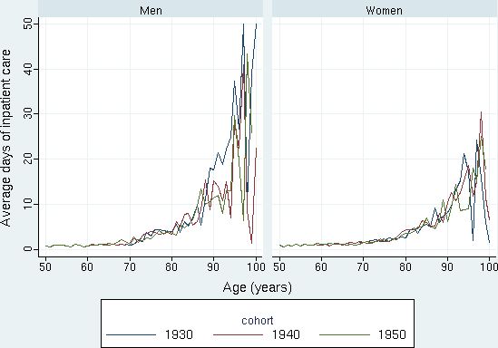
Simulated average days of inpatient care by age 50-100 for the birth cohorts of 1930, 1940, and 1950. Men and women, respectively. Source: Figure 10.2 in Bolin et al. (2008c).
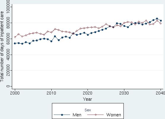
Figure 4 displays the evolution of the total number of inpatient days by gender until 2040.

Simulated development of total number of days of inpatient care for the total Swedish population, by gender. Source: Figure 10.7 in Bolin et al. (2008c).
3.5.4. Models for retirement
The retirement models distinguish between retirement with disability pension and with old-age pension. The former is considered primarily driven by ill health, while old-age pension is at least partly driven by economic incentives. Individuals who have been ill for a long time and are unable to work can get disability pension. At the age of 65 it is automatically turned into old-age pension. The typical pension age in Sweden is 65 and the pension systems have been designed such that people normally will retire at this age. It is though usually possible to take an early pension already at 61, but at a reduced compensation rate. The Swedish pension system has three “pillars”: the social security pensions which usually give a compensation rate at about 60 percent; the occupational pensions which give another 10 per cent for most retirees, and private pensions which are equivalent to private savings.
Before September 2001 most employees had to retire no later than at the age of 65. Contracts between employers and unions gave the employers right to discontinue the employment contract for those who reached this age. Parliament has now taken a law which shifts this threshold up to 67. The peak age of retirement is still 65, however. The old contracts and social conventions thus determine this peak, while early retirement is a decision subject to economic incentives.
Early retirement via the disability insurance was modeled using a discrete choice model (Bolin et al., 2008b). The choice of explanatory variables reflects our view that exit from the labor market via the disability insurance is involuntary and determined by the health status. The explanatory variables thus capture health risks rather than economic incentives.
The literature on retirement suggests a few different approaches to model old-age retirement, see for instance the discussion in section 4 of Bolin et al. (2008b). We might distinguish between the life-time budget constraint approach, the option value approach and the hazard model approach. In the life-time budget constraint approach each individual faces a discontinuous or kinked life-time budget constraint and is assumed to choose the retirement age which gives the utility maximizing combination of leisure and life-cycle income. In the option value approach each individual is assumed to compute the expected gain (loss) in utility from postponing retirement one or more years. The hazard model approach is a reduced form approach which usually only considers information one period ahead. The probability to retire for a person who is currently active is typically a function of annual wage earnings, pension accruals and pension wealth, health status, age and gender.
The first two approaches are very computer intensive, and for this reason difficult to include in a microsimulation model. Even with modern fast computers simulations would take too long. The limited information available in SESIM and its intrinsic chronological structure also contributed to our decision to use a discrete choice model for early old-age retirement as well as for retirement via the disability insurance.
When looking at data the research group discovered that some individuals, who retired before 65, got a higher pension than their contracts stipulated. A closer analysis of the retirement situation revealed that some employees, typically in the age bracket 55-65, got early retirement offers from their employers, so called “golden handshakes”. This was a way to get rid of white-collar employees and reduce the expenses for both salaries and pension contributions, which tend to increase with increasing age. To estimate a discrete choice model for the private decision to retire without taking these offers from employers into account would in general bias the estimates. For this reason, a model for the probability to get an offer was also estimated and made part of the entire model structure.
When simulating the retirement model, we start with withdrawal through the disability insurance. The population at risk consists of everyone in the labor force. After those who are simulated to get disability insurance have been dropped from the labor force, those who remain are at risk for early old-age retirement. Those who remain in the labor force at the age of 65 are all assumed to retire at that age. The model can be simulated with and without early retirement offers from employers. It is also possible to extend the age span for market work beyond the age of 65.
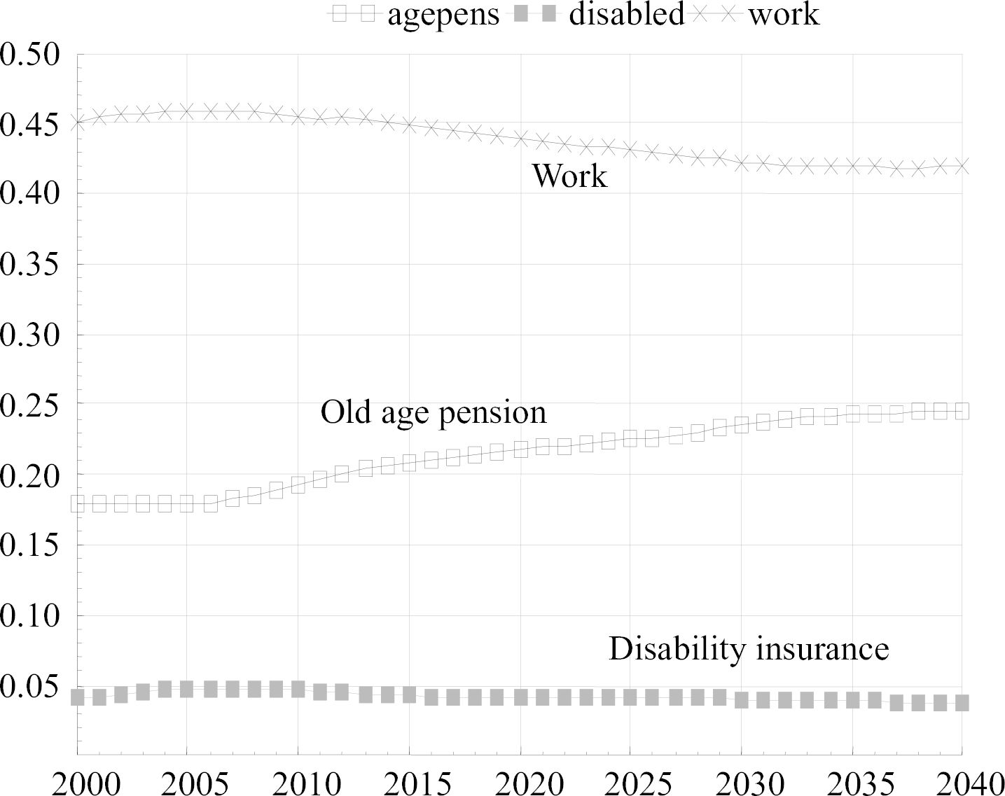
Figures 5 and 6 give examples of simulation output. The first of these figures show the simulated population shares in work, old-age retirement and on disability insurance from year 2000 to 2040. The share in old-age retirement will increase from about 18 per cent in 2000 to about 25 percent in 2040, while the share in work decreases from 45 per cent to 42 per cent. The marginal decline in the share of disability insurance is probably the combined result of population ageing and the fact that disability insurance is converted into old-age pension at the age of 65.

Simulated population shares in work, retirement and disability; all age groups. Source: Figure 5 in Bolin et al. (2008b).

Average transition age to old-age retirement by gender using two alternative scenarios. Source: Figure 10 in Bolin et al. (2008b)
Figure 6 displays the evolution of the average retirement age under two alternative scenarios. One is the base scenario when everyone is assumed to go into old-age retirement no later than at the age of 65. The alternative scenario extends this age limit to 70. In the first case the average retirement age remains at a level just below 64 years. In the alternative scenario the retirement age grows to a steady state between 66 and 67 years.
3.5.5. Models to simulate the evolution of the distribution of wealth
When simulating the evolution of the distribution of wealth it is not possible to use a conventional portfolio allocation model that can be estimated from a single cross-section of data. Such a model would give too much volatility in the simulated data. We needed a model which uses information about the stock of assets last year and then simulates any changes. We also needed a model which at least distinguishes between owner occupied housing, tax-deferred pension savings, study debts, other debts and other assets, because taxes and benefits would depend on this categorization. From an analytical point of view, it might have been desirable also to distinguish between risky and less risky assets, and one might also have preferred to distinguish between mortgages and consumption credit. Data limitations and the fact that the main focus of our study did not require a detailed brake down of financial assets made us settle for the following groups of assets: owner occupied housing, other real estate (mostly vacation houses, farm- and forest properties, and apartment complexes), tax deferred pension savings, other financial asset, study loans and other debt.
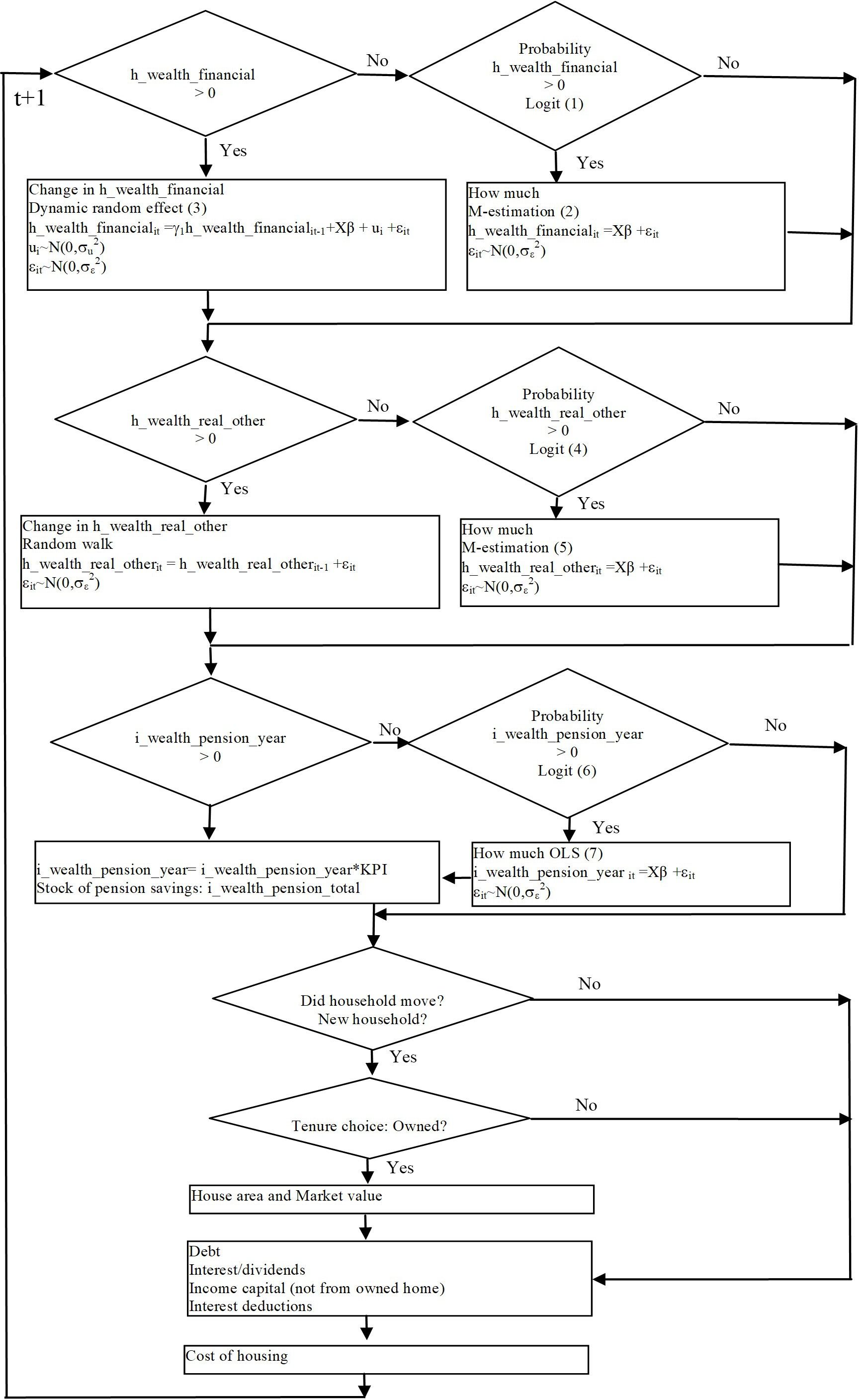
The distributions of these assets are heavily skewed, and many households do not hold all of them. One has to consider these properties of data when formulating and estimating models, so the simulated distributions are able to replicate them. Figure 7 gives a view of the model structure and the simulation path. Financial wealth precedes real wealth and debts because if a household has financial assets, it might influence any decision about buying new property and taking up debt. The model also systematically distinguishes between those who have an asset and those who do not. In the first case a dynamic model is applied, while in the second a two-part model is used. The two-part model includes a discrete choice model which determines the probability to acquire the asset and a regression type of model which determines the amount acquired. Most of these models were estimated from longitudinal LINDA data.

Financial and real wealth and cost of housing in SESIM. Source: Figure 1 in Flood and Klevmarken (2008).
Our efforts to estimate a dynamic model for other real estate were not successful. The process was dominated by few but rather large changes in holdings and it turned out that a simple random walk replicated observed data as well as any model we could come up with. Owner occupied housing was treated somewhat differently. A geographical move implies new housing and for this reason decisions to buy a new house or an apartment were modeled and simulated jointly with these moves. Also households which remained in the same area were exposed to a nonzero risk of buying new housing. If a household was simulated to buy a new house or an apartment the market value of the property was simulated as a function of geographical area, floor area, financial wealth, income and demographic variables. This is thus a reduced form relation capturing both the two most important supply variables (geographical area and floor size) and demand variables (wealth, income and family type)
Study debts are loans offered to college and university students by the government. We assumed that the take up rate was 100 per cent and that students borrowed as much as they were allowed to do. Study debts are increased by a certain interest rate determined by the government, and repayments of principal and interest depend on the former student’s income according to rules programmed into SESIM. Thus, no stochastic model was thus applied in this case.
To model changes in other debt than study loans was not that simple because the distribution of change in debt had rather fat tails. For instance, the median change was 0 and the mean 13 000 SEK, while the largest observed increase was 77 millions and the largest decrease 97 millions! The final decision became to estimate a sequence of models: A random effects probit model for the probability of taking up a loan if the household had no loan previously, a random effects GLS regression of the logarithm of new debts given that the household had no debt in the previous year, a random effects probit model for the probability to stay in debt, and a random effects GLS regression of the logarithm of debt for households that continue to have debts.
All models were estimated with data at the 1999 price level, and all simulations were also done at this price level. Afterwards assets and debts were inflated by exogenously imputed interest rates and price increases on real property.
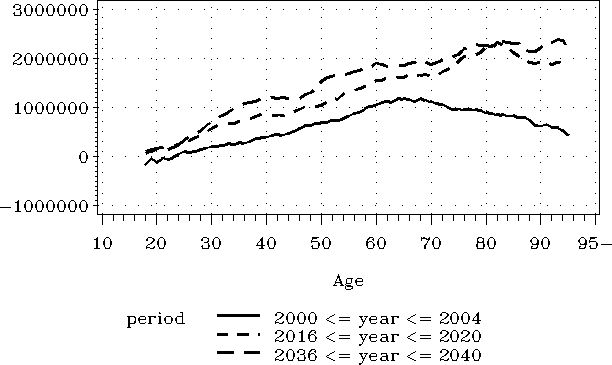
Figure 8 gives an example of the results of these simulations. The average cross-sectional age-wealth profile for the years 2000-2004 shows the well-known reversed U-shape with a peak at about 65. The simulations then show that the peak moves to the right and disappears at the end of the simulation period.

Mean net wealth by period and age of the oldest in the household (SEK in 1999 prices). Source: Figure 3 in Flood and Klevmarken (2008).
3.5.6. Simulation results
Our basic simulation scenario includes certain assumptions about the macro indicators which are fed into the model exogenously. For the period 1999-2004 we have used observed values. After 2010 the following assumptions apply:
Annual rate of change in inflation (CPI): 2.00 %
Annual average increase in real wage rates: 2.00 %
Short-term interest rate: 4.00 %
Long-term interest rate: 5.00 %
Dividends: 2.50 %
Rate of change in prices of stocks and shares: 3.75 %
The market value of single-family houses: 3.50%
For the period 2005-2010 these rates were allowed to adjust from the last observed rate to the constant rates above. Demographic changes were aligned to the basic predictions from Statistics Sweden and the average unemployment rate was aligned to the medium-term forecasts from the Ministry of Finance.
In addition to this basic scenario, we have run a number of alternatives to investigate the sensitivity of the results and explore policy alternatives. They will be explained below at the same time as key simulation results are explained and commented.
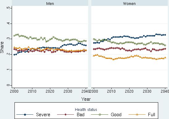
Let us start with the health status of the population, which is measured with an index based on self-reported health and self-reported ability to carry out work and other tasks. It takes on four values ranging from full health, good health and bad health to severe health. The simulations show a marginal decline in health status among the elderly as we approach year 2040. In the age bracket 50-74 the share with severe illness increases from 7 per cent to 10. Among women who are 74+ the share increases from about 28 per cent to 35. The health of the oldest men also decreases a little but not as much as for women. (See Figure 9!) These changes reflect the observation that the current health status among young adults is somewhat less than it was for the same age group of previous cohorts, due to for instance, increased obesity, allergies and mental problems.

Simulated health status 2000-2040 for people aged 75+. (Population shares by health status and year.). Source: Figure 13 in Bolin et al. (2008a).
The increased number of elderly and the (marginal) decrease in health status will increase the demand for health care. The first panel of Table 5 shows that the average number of days in hospital per year and person 65+ will increase marginally. This is a result both of the increase in the average age of this group and of the decrease in health status. The table also shows the result of two alternative scenarios. First, we increased the health progression of the elderly by adjusting the health index for those aged 40-90 proportionally to their age minus 40 and the calendar year minus 2000 in such a way that a 90-year-old person in 2040 will have the same health as an 80 years old in the base scenario. This implies that the improvement in health comes gradually and is largest for the elderly. The result was that the average number of hospital days was simulated to decrease rather than to increase. In this scenario the death rates were, however, kept at their old age-specific values. If health status increases one might expect that the death rates would decrease. For this reason, the third scenario combines the increase in health status with a decline in age-specific death rates. After year 2010 and after the age of 35-40 each individual was assumed to have the death risk of a 5-year younger person in the base scenario. To avoid excessively old persons the death risks after the age of 100 was eased upwards towards the levels of the base scenario. The result is a rather dramatic increase in the average number of hospital days. The explanation is that we get an agglomeration of very old persons at the end of the simulation period.
Average and total number of inpatient hospital days for people 65+ by year.
| Year | Average no of days | Total no of days (1000) | ||||
|---|---|---|---|---|---|---|
| Base scenario | Improved health | Improved health & lower death risks | Base scenario | Improved health | Improved health & lower death risks | |
| 2000 | 3.2 | 3.3 | 3.2 | 4954 | 5068 | 4990 |
| 2020 | 3.2 | 3.1 | 3.5 | 6495 | 6270 | 8117 |
| 2040 | 3.4 | 2.9 | 4.0 | 8396 | 7241 | 12087 |
-
Source: Table 3 in Klevmarken (2008b).
The second panel of Table 5 shows the combined effects of the change in the average number of days and the population increase in the age segment 65+. The total number of days in hospitals for people 65+ will in the base scenario increase by about 70 per cent, in the improved health alternative only by 43 per cent, and when the death rates decrease the number of hospital days increase by as much as 142 per cent. The assumed decrease in death rates might be exaggerated, but these simulations show that the results are rather sensitive to the death rates. If the health status of the population improves such that people survive to very old age, but they then will be in need of much health care, we will in the future experience an explosive increase in demand for health care from the old-old.
We will also expect an increase in social care of the elderly. Figure 10 shows the simulated number of elderly with around-the-clock care for the period 2000-2039 by age group in the base scenario. We find that the number of old people who get this kind of institutionalized care will increase from about 70 000 to 160 000. It will increase in all three age groups but most among the very old. There are similar but not quite as dramatic changes for home help, see Figure 11.
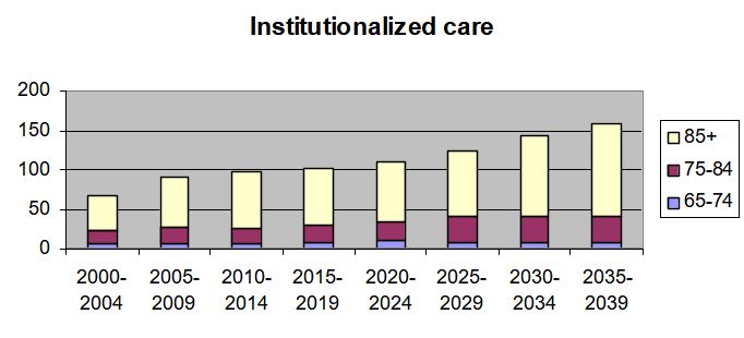

Total number of elderly with around-the-clock care 2000-2039 (1000s). Source: Figure 6 in Fransson et al. (2008).
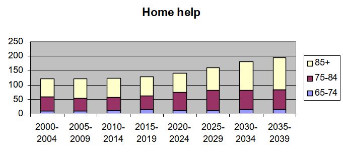

Total number of elderly with home help 2000-2039 (1000s). Source: Figure 6 in Fransson et al. (2008).
Using data on average cost per person and hospital day and annual averages per person for institutionalized care and home-help, and the assumption that these numbers will increase by the average increase in the real wage rate, we have computed total expenditures for these three forms of care, see Table 6. The table gives estimates for three years. We find that the total will increase in real terms by a factor of 3.6. To understand how much this is we should have been able to simulate the future budget for the public sector, but SESIM is not able to do it. The model, however, simulates how much everyone pays in direct taxes, and we have thus put the total of these expenditures relative to the sum of all direct taxes from the household sector. The result is displayed in the second column of Table 6. We find that the expenditure share will increase from about 20 per cent in 2000 to 36 per cent in 2040. This suggests that the increased expenditures for health care and social care due to population ageing will become an increased burden to the public budget.14
Total expenditures for inpatient care, home help and institutionalized care for people 65+.
| Year | Total expenditures (millions of SEK in fixed prices) | Total expenditure as share of the sum of direct taxes from households (%) |
|---|---|---|
| 2000 | 92231 | 20.5 |
| 2020 | 166719 | 24.9 |
| 2040 | 339297 | 36.2 |
-
Source: Table 6 in Klevmarken (2008b).
Let us now turn to the income and wealth of the elderly. Figure 12 shows the simulated average taxable income for retired relative to the average taxable income of the working cohorts of age 20-64 for a few selected birth cohorts as they age. Everyone is assumed to retire no later than at the age of 65. At this age relative income lies in the interval 75-80 per cent. As the elderly age, their relative income decreases. The drop in income around the age 70 is a result of our assumption that the funded components of the pensions are paid out during the first five years. An individual can choose to have them paid out for a longer period or life-long. Had we chosen such an alternative the kink at age 70 had been smoothed. We find that the relative income of these cohorts decreases down to about 50 per cent at the age of 80. The explanation is that the pension system is “front loaded”. Pensions are indexed by a wage rate index to make them follow the income changes of an average worker, but each year 1.6 percentage units are subtracted, which implies that the income standard of the elderly will deviate more and more from that of workers as the elderly age. We might also note that the curves of the older cohorts lie higher than those of the younger. The main explanation is that the younger cohorts will on average live longer and their pensions will thus have to be paid out for a longer period. Their annual pension will then have to decrease, unless they retire later.
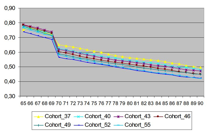

Average taxable income for retired relative to the average taxable income of working cohorts aged 20-64, by birth cohort and calendar year. Source: Figure 11 in Flood et al. (2008).
Because the group 65+ age and because younger cohorts get relatively lower pensions the relative income of the whole group 65+ will decrease. This is seen in Table 7, but for a different income concept – equivalized disposable income. Relative income decreases from about 70 per cent in 2000 to about 55 per cent in 2040 in our base scenario. If we allow people to work in the market until the age of 70 the situation improves. Relative income then only drops to about 62 per cent. The explanation is that the group 65+ will have market incomes, which are higher than pensions, for a few more years, and that the pension will be paid out during a somewhat shorter period.
Median equivalized disposable income of 65+ relative to the median income of 20-64, by year in two scenarios.
| Year | Base scenario | High pension age |
|---|---|---|
| 2000 | 0.709 | 0.711 |
| 2020 | 0.634 | 0.693 |
| 2040 | 0.552 | 0.623 |
-
Source: Table 13 in Klevmarken (2008b).
The low relative income at the end of life raises the issue of poverty. We have defined poverty as having an equivalized disposable income less than 50 per cent of the median of the adult population. Figure 13 shows the poverty rate for a few cohorts as they age. It is very low among working age people, just a few per cent, but increases a few years before the typical retirement age of 65. In the age group 55-65 there are relatively many on disability pension and on early old-age pension, which are relatively low. Immediately after 65 the poverty share goes down because the general old-age pension with a guaranteed minimum raises the income standard. As people grow older the poverty rate increases because their relative income standard decreases as demonstrated above. The youngest cohorts have the highest poverty rate for the same reason that they have the lowest relative income. When they get into the 80:s the poverty rate gets as high as 20 per cent.
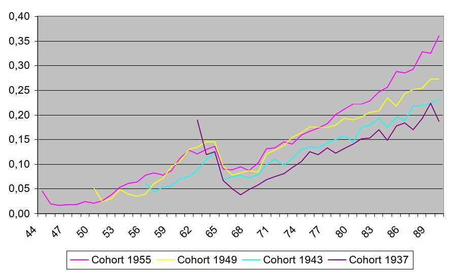

Poverty share by birth cohort and age (equivalized disposable income less than 50 % of the median income of the adult population). Source: Figure 14 in Flood et al. (2008).
The resources of the elderly are not only determined by their pensions and other incomes but also by their assets. The baby boom cohorts are relatively wealthy, a wealth that could be liquidized and used for consumption, health care and social care. In SESIM we have simulated the evolution of the wealth distribution and we have already seen a snapshot of the results in Figure 8. The simulations show that the peak is pushed to the right and up, and at the end of the simulation period there is almost no peak at all. The curve is an increasing trend. This implies that SESIM simulates that the elderly will keep their wealth rather than to consume it. The shift in the peak is not just an artifact built into SESIM. It can be observed in data, see Figure 1 in Klevmarken (2006).
An important social policy issue is if those in most need of care will have income and wealth that could cover their expenditures for these services, or if the neediest also are those with the smallest resources. In SESIM we can distinguish between those who use care services and those who do not, and we can also see what income they have and how wealthy they are. Table 8 responds to the question: “What income do those in most need of care have?”
What income do those in most need of social care have? (Per cent of all 65+ in each form of care.).
| Year/Kind of care | Quartiles of the distribution of disposable income for all adults | ||||
|---|---|---|---|---|---|
| 1 | 2 | 3 | 4 | All | |
| 2000 | |||||
| No care | 46.7 | 30.8 | 14.1 | 8.4 | 100 |
| Home help | 68.6 | 18.7 | 7.1 | 5.6 | 100 |
| Institutionalized | 65.5 | 22.2 | 8.0 | 4.3 | 100 |
| 2040 | |||||
| No care | 53.1 | 30.7 | 10.9 | 5.3 | 100 |
| Home help | 75.4 | 17.6 | 3.8 | 3.2 | 100 |
| Institutionalized | 76.4 | 14.7 | 4.6 | 4.2 | 100 |
-
Source: Table 17 in Klevmarken (2008b).
Most elderly belong to the first or second income quartile. In year 2000 46.7 per cent of those who did not use any social care belonged to the first income quartile, ie the 25 per cent with the lowest incomes, while as much as 65-70 per cent of those who used public social care belonged to the same quartile. Our simulations suggest that the situation will become even worse in 2040. By then 75 percent of those who use public social care will belong to the first income quartile. These results suggest that those who are in need of public social care will not have the incomes needed to pay for these services, either privately or by increased taxes.
Table 9 shows, however, that the elderly are relatively better off in terms of wealth. In 2000 40 per cent of those who did not use any care belonged to the 4th quartile and about 30 per cent of those who used home help or were institutionalized. Only a few per cent belonged to the first quartile. In 2040 the inequality of the distribution is simulated to increase, the population shares in the first and fourth quartiles increase.
How much wealth do those in most need of care have? (Per cent of all 65+ in each form of care).
| Year/kind of care | Quartiles of the distribution of net worth for all adults | ||||
|---|---|---|---|---|---|
| 1 | 2 | 3 | 4 | All | |
| 2000 | |||||
| No care | 4.7 | 28.0 | 27.4 | 39.9 | 100 |
| Home help | 2.5 | 40.2 | 27.4 | 29.8 | 100 |
| Institutionalized | 2.0 | 39.9 | 25.8 | 32.3 | 100 |
| 2040 | |||||
| No care | 12.0 | 17.4 | 20.8 | 49.9 | 100 |
| Home help | 12.4 | 20.1 | 18.2 | 49.3 | 100 |
| Institutionalized | 11.1 | 21.6 | 19.9 | 47.4 | 100 |
-
Source: Table 18 in Klevmarken (2008b).
From these results it is obvious that we will get a rather large group which is income poor. Some of them will however have some wealth, but that is not true for everybody. At the end of the period the share of the elderly that will both have low incomes and no wealth is simulated to increase. Table 10 shows more specifically the poverty rate among the elderly when we define poverty as having an equivalized disposable income less than 50 per cent of the median equivalized income of the entire population and an equivalized net worth less than 50 per cent of the median equivalized net worth of the whole population. Simulation results are shown for the base scenario and when the maximum pension age is increased from 65 to 70 years. In 2000 the poverty rate was low, about 1.6 per cent for all elderly 65+. It was about 1 percentage unit higher among institutionalized elderly. According to the base scenario these numbers will increase to 2040. The poverty rate for all elderly is simulated to become 14.5 per cent and for those who use social care one or two percentage units higher. If the maximum pension age is increased and people chose to retire later the poverty rate will not increase as much. In our alternative scenario we would get about 8 per cent poor among all elderly and among the institutionalized about 12 per cent would become poor. These numbers are also sensitive to our growth assumption. Higher growth and lower unemployment will reduce poverty while lower growth and higher unemployment will increase it, see Klevmarken (2008b) Table 20.
Poverty rates among people aged 65+, by type of assistance, year and scenario (%).
| Scenario/year | Type of assistance | |||
|---|---|---|---|---|
| No assistance | Help at home | All day Surveillance | All 65+ | |
| Base scenario | ||||
| 2000 | 1.5 | 1.4 | 2.5 | 1.6 |
| 2020 | 11.1 | 10.8 | 13.2 | 11.2 |
| 2040 | 14.3 | 15.1 | 16.3 | 14.5 |
| Increased pension age | ||||
| 2000 | 1.7 | 2.6 | 2.2 | 1.8 |
| 2020 | 6.8 | 7.2 | 10.1 | 7.0 |
| 2040 | 7.9 | 9.8 | 12.0 | 8.3 |
-
Source: Table 20 in Klevmarken (2008b).
These results suggest that we will get a relatively large share of elderly who will not have the means to pay for the health and social services they will need. Today family members and kin provide a large share of the help to elderly. Wives in particular help their husbands and daughters help their old mothers. Will this resource be available also in the future and help to ease the expected increased pressure on the public sector? To answer this question we have simulated the domestic migration between different parts of the country and measured how closely children live to their parents. A necessary condition for being able to help one’s parents on a more regular basis is that the child lives within commuting distance to the parent. Figure 14 shows how the share of elderly who live in commuting distance from the nearest child will decrease. The explanation to this result is that geographical mobility has increased. Young people move to get education and never return home, and young people also leave the rural areas and move into the major metropolitan areas, where it is easier to find a good job. When we looked more closely at the numbers behind Figure 14 we found that the share of single fathers and mothers who lived close to their children was smaller than the share of couples. Unfortunately, singles are in more need of help than couples. Our simulations thus suggest that we cannot expect children to do more for their parents than they already are. On the contrary, they can rather be expected to do less.
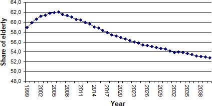

Share of elderly living close to adult children. Source: Figure 2 in Fransson et al. (2008).
3.5.6. Conclusions
If the same share of elderly as currently will get access to health care and social care in the future, the supply of these services would have to increase at the same rate as the age groups concerned. (Inpatient care by 70 per cent, home help by 50 per cent and institutionalized care by 80 per cent.)
The expenditures for these services tend to increase faster than the tax revenues from households. This will imply reallocation of resources within the public sector, higher taxes or increased user-fees.
The income standard of those who are retired will decrease as they age relative to the working generations. Younger birth cohorts will get lower relative incomes than older cohorts unless they retire later.
A large share of the very old will get so low incomes that they become poor. This group will not have the means to pay for care.
The baby boom cohorts of the 1940s are relatively wealthy and they will according to our simulations keep their wealth also when they age. This is a potential source to fund increasing care expenditures, but a large share of this wealth is tied up in housing.
We will, however, have a relatively large group of care needing elderly who both have low incomes and very little wealth. This group will not be able to afford higher charges for care.
We should not expect that children and other relatives step in and substitute for public care.
Increased immigration is not very effective in balancing the increased burden of care for our elderly.
Much more effective is an increase in the average retirement age, the ability to maintain high economic growth and good public health.
Our simulations are sensitive to changes in the death rates. Low death rates for “young old” may - depending on the health status of the elderly – result in an increasing number of very old and heavily care dependent persons.
4. Concluding evaluation of advantages and short comings of SESIM
A model is built to respond to certain scientific problems, or to policy problems. There is no model which can respond to all our problems, now or in the future. The design of a model is determined by its applications. This is true for microsimulation models as well as for other models. In the case of SESIM it was originally designed to analyze the properties of the Swedish student grant and loan system. It was then added to for studies of the properties of the pension system and finally further expanded for a study of the consequences of population ageing. In this gradual expansion of the model more and more submodels have been added to SESIM, such that it today can respond to more questions than its first version could. Is there any limit to the possibilities to add new structures and refine old ones? With unlimited time and resources, perhaps not, but in practice neither time nor resources are unlimited. In policy applications time might be the binding constraint, because policy makers have to take decisions and they need the output from a simulation in time for the decision, while in scientific work resources might be the binding constraint. But the key issue is what properties a model must have to answer a particular policy question. If it is possible to get an intelligent answer from a small model, why use a large and complex one?
The idea behind microsimulation is to model the decisions of those who actually make them, not the make-believe decisions of aggregates of decision makers. In SESIM the unit of analysis is thus the individual and the household. Another important idea is that the model should include the policy instruments that the policy makers actually use, for instance the true eligibility rules for tax deductions and all the details of the tax scales rather than just an average tax rate. SESIM thus includes (almost) all the details of the Swedish personal tax system, social security system and other benefits to the household sector. The model aims at capturing both individual longitudinal trajectories and cross-sectional distributions. Usually, it is of interest to study both the snap-shot of poverty a cross-sectional distribution gives and to understand for how long people stay in poverty. To accomplish this we need both a demographic model that can age and renew the population and dynamic behavioral models which tell us when people take their decisions.
The basic time unit in SESIM is a calendar year. Most simulations are designed to replicate what happens to an individual in a year. One reason for this is that the tax system operates on an annual basis. There are, however, processes which run on a shorter time span. For instance, sickness benefits are given by the day and unemployment compensation by month and day. In these cases we simulate the number of days (months) with benefits within a year, but not when in a year the spells of sickness or unemployment take place. Mostly for practical reasons the model and the simulations have a hierarchical structure. We try to simulate in an order such that decisions which have immediate far-reaching consequences come first in the simulation sequence. This does not necessarily imply that individuals take decisions in this order. In principle one can think of joint decisions, and to some extent it might be possible to model some decisions as joint decisions, but it is hardly practical (or even realistic) to model all decisions in a year as joint. How the model is specified in this respect does not only have implications for the simulations but also for the estimation of the submodels. Models of joint decisions will in general have to be estimated jointly, while models which form a block recursive structure can be estimated recursively.
There are a number of shortcomings of the current version of SESIM. One is that there is no proper labor supply model. There are models for labor force participation, unemployment and retirement, but no model that simulates the number of hours worked, and the only model which has economic incentives built into it is the model for old age retirement. We have run experiments with decreased marginal income tax rates, but the effect of such changes on labor supply and retirement is unrealistically small. SESIM would thus become more useful if it could simulate the annual number of hours worked as a function of the budget set each individual faces. However, the labor supply model cannot be a conventional model of Hausman type. Such a model would give too much mobility in hours worked. We need a model which conditions each individual’s decision on current and possibly past work hours.
Another shortcoming is that there is no functional relationship between health status and death rates. We have experienced that the public expenditures for health care and social care for the elderly depend very much on the death rates. I the life span increases but the age specific health status among the elderly does not improve, we will get an agglomeration of elderly in need of expensive care. It is thus important to understand how health as young and middle-aged influences the health status when people reach a high age, and how changes in health influence the age specific death risks. We would also like to understand better how changes in the economic incentives to work longer will influence the health status of the elderly.
A special problem when modeling the utilization of publicly provided services is that there is no regular market for these services. The fees the users pay are kept artificially low and if there is excess demand access is usually regulated in a queuing system. Changes in utilization will then be determined by political decisions to increase supply. The relations we estimate become a mixture of supply and demand although the models usually are specified as if they were demand models. Simulations are then done using the assumption of unchanged policy.
Still another shortcoming is the absence of market feedback and macroeconomic feedback. SESIM is a model for the household sector, and it does not include any balancing market mechanism. Changes in the macro environment can be fed into the model exogenously but there is no general equilibrium mechanism built into the model. When modeling domestic migration and the demand for housing we considered introducing a price mechanism for owner occupied houses, because the model carries the current migration pattern forward, and it implies that an increasing share of the population will live in the three big cities. This should result in an upward pressure on the real estate prices in the cities, which could counteract the migration flow. Such an increase in real estate prices would also imply a continued shift in wealth from the rural areas to the big cities. For various reasons the introduction of a price mechanism for owner occupied homes was, however, deferred to the future.
As explained in section 3.3 the Ministry of Finance used a macro model to simulate the complete public sector parallel to the household sector of SESIM. The literature also gives a few examples of attempts to integrate a CGE model with a microsimualtion model. These attempts are, however, still experimental. A badly specified CGE model might destroy the microsimulation results. A cautious approach to introduce market feedback is to do it in specific markets as suggested above, and gradually work in the direction of a macro model.
Model building must be based on theory, whether economic theory or theory from another field. Many economic models are of the “ceteris paribus” kind, focusing only on the key phenomenon they were designed to explain, but ignoring much of the complexities that generated data. Such desktop models are not ideal instruments in microsimulation. A model built for simulation should use all the information available at the start of the simulation. As one of the objectives of SESIM is to simulate longitudinal trajectories its models must have a memory. Models which can be estimated from single cross-sections and implicitly assume that new decisions are taken every year independently of past history, will tend to exaggerate mobility. Furthermore, simulation models should be able to simulate the whole distribution of its endogenous variables, not just conditional means. This has implications both for the choice of model structure and in principle also for estimation. For instance, a nonstandard residual structure might hide heterogeneity in behavior; ie the population might consist of several subpopulations that behave differently. A possible solution is then to estimate one model for each subpopulation. An advantage with microsimulation is that heterogeneity of this kind is relatively easy to build into the model.
In SESIM calibration is used to align changes in the simulated demography to the official forecasts of Statistics Sweden (2009), to make the model follow exogenously given paths of certain key variables, such as the rate of unemployment, and to reduce simulation volatility. All these uses have good motivations. Calibration can for instance be a good way to impose alternative exogenous assumptions on the model. But calibration can also be misused if it forces the model into a track it had (almost) never gone into without calibration. Calibration can be viewed as a form of constrained estimation. If the constraints are rejected by the model, enforcing them will in general lead to biased simulations.
Data shortage is usually a severe constraint when building a microsimulation model. SESIM has the advantage of the large and rich micro data of LINDA. A special advantage is that this data source includes exactly the same data used by the tax and social security authorities in computing taxes and benefits. Never-the-less we found it necessary to use complimentary data sources in particular for the health and care models and for geographical mobility. In all cases the unit of analysis – an individual – was the same and many variables were also defined in the same way in all data sources.
Because the simulated values come from a stochastic model estimated from sample data they are uncertain. The stochastic uncertainty originates from three sources: the sample which constitutes the population of SESIM, the estimates of the model parameters and the stochastic structure of the model. The population of SESIM is so large that data uncertainty and simulation uncertainty usually are no problem. Only for small subgroups of the population and in the extreme tails of distributions these sources of uncertainty might become a problem. How much errors in the estimated parameters contribute to total uncertainty is something which still remains to be investigated.
The more we add to a microsimulation model the more difficult it becomes to understand what the model is doing, why it produces the results it does. Depending on the model structure a large model increases the risk that systematic errors from badly specified submodels spread through the entire model. On the other hand, a simulation model like SESIM must capture all important mechanisms that determine our observations. To a degree complexity cannot be avoided. But economic models are still rather small compared to models used in other disciplines, and economists have to learn how to work with large models. How one by using simulation techniques can evaluate the properties of a large model and test it against data.
Are we ready to use large scale microsimulation models for policy advice? I hope the examples I have given in this paper show the potential. If we have the resources needed and are willing to follow rigorous scientific procedures microsimulation is a powerful tool in policy evaluation. It is not one man’s work to build a microsimulation model. Depending on the policy problem one usually needs a team of specialists from different fields. It is also important to have a rather long perspective: When the first version of the model is built who will update it as tax laws and the benefit rules change, who will test it against new data, who will reestimate the behavioral relations and add new submodels, who will evaluate its properties? A successful microsimulation project needs a scientific environment with continuity and resources that most university departments do not provide.
Footnotes
1.
If the sample was not just a simple random sample but obtained by a more complex sampling design, the corresponding design weights are used to get an inference to the entire population. In practice when the sample is a few years old, it is also common to reweight the sample to compensate for demographic and other structural changes that have taken place since the sample was drawn.
2.
The LINDA data base only includes administrative register data. There is thus no problem of attrition.
3.
For a description of the methodology used se Flood (2008)
4.
Alignment can be achieved by adjusting the parameters of the model such that the known totals are replicated. This can be seen as estimation subject to side constraints, see Klevmarken (2002) and Klevmarken (2008a). But estimating a misspecified model subject to correct side constraints will in general result in estimates which have a misspecification bias.
5.
Today a regular student gets about 6000USD (4000 euro) for fulltime studies in two semesters (40 weeks). About 33 per cent is a cash benefit and the rest a loan which has to be repaid with interest.
6.
After 2001 stricter rules for repayment was enforced.
7.
Occupational pensions typically add about 10 percentage units to the compensation rate.
8.
However, it is not obvious that a CPI can be used in a meaningful way for such a long time period as a life-time.
9.
This implies that the consumer’s utility depends on the consumption of other individuals. Increased utility is only attained if one’s own consumption increases more than that of other consumers.
10.
Average disposable income after retirement relative to the average disposable income in the five last years before retirement. Computations were limited to individuals who had worked at least five years before retirement and survived at least ten years after retirement.
11.
Source: Sveriges framtida befolkning 2006-2050, Demografiska rapporter 2006:2, Statistics Sweden
12.
In this paper the terminology “young-old” and “old-old” will be used to characterize people between 65 and 75(80) and above 75(80), depending on context.
13.
Population ageing in Japan is extreme. According to the U.N. World Population Prospects (The 2008 revision) The old-age dependency ratio of year 2000 was 0.42 while the prediction for 2050 is as high as 1.09! Please note that dependency ratios are sensitive to the choice of age groups. For instance, if one defines dependency as the ratio of 65+ to those 15-64, the figures for Japan become 0.25 and 0.74 respectively, while those for Sweden are 0.27 and 0.41.
14.
Expenditures for medicine have not been included in our computations. It is difficult to predict the future of these expenditures. In the period 2000-2008 total nominal expenditures for medicine increased by almost 5 per cent per year.
References
-
1
Changes in the Health Status of the PopulationChanges in the Health Status of the Population, Chapter 4 in Klevmarken and Lindgren 2008.
- 2
-
3
Utilization of Inpatient CareUtilization of Inpatient Care, Chapter 10 in Klevmarken and Lindgren 2008.
-
4
Studiebidraget i Det Långa Loppet, Expertgruppen För Offentliga Studier (ESOStockholm: Finansdepartementet.
-
5
Modelling Our Future: Population Ageing, Social Security and TaxationAmsterdam: Elsevier B.V.
-
6
SESIM: A Swedish Micro-Simulation ModelSESIM: A Swedish Micro-Simulation Model, Chapter 3 in Klevmarken and Lindgren 2008.
-
7
The Distribution of WealthThe Distribution of Wealth, Chapter 9 in Klevmarken and Lindgren 2008.
-
8
The Income of the Baby BoomersThe Income of the Baby Boomers, Chapter 8 in Klevmarken and Lindgren 2008.
-
9
The Demand for Old Age CareThe Demand for Old Age Care, Chapter 11 in Klevmarken and Lindgren 2008.
-
10
The Distribution of Wealth in Sweden: Trends and Driving Factors29–44, The Distribution of Wealth in Sweden: Trends and Driving Factors, Vol, 10, Band, Wirtschaftswissenschaftlige Tagungen der Arbeitskammer Wien, p.
-
11
Simulating an Ageing Population. A Microsimulation Approach Applied to Sweden. Contributions to Economic Analysis No 285Bingley, UK: Emerald Group Publishing Lmtd.https://doi.org/10.1016/S0573-8555(2008)285
-
12
Statistical inference in micro-simulation models: incorporating external informationMathematics and Computers in Simulation 59:255–265.https://doi.org/10.1016/S0378-4754(01)00413-X
-
13
Dynamic Microsimulation for Policy Analysis: Problems and SolutionsDynamic Microsimulation for Policy Analysis: Problems and Solutions, Chapter 2 in Klevmarken and Lindgren 2008.
-
14
Simulating the Future of the ElderlySimulating the Future of the Elderly, Chapter 12 in Klevmarken and Lindgren 2008.
-
15
Chapter 8Lifetime Redistribution Through Taxes, Transfers and Non-Cash Benefits, Chapter 8, Modelling Our Future: Population Ageing, Social Security and Taxation, Amsterdam, Elsevier B.V.
-
16
Generationsanalyser – Omfördelning Mellan Generationer i En Växande Välfärdsstat, Finansdepartementet, Expertgruppen För Studier i SamhällsekonomiGenerationsanalyser – Omfördelning Mellan Generationer i En Växande Välfärdsstat, Finansdepartementet, Expertgruppen För Studier i Samhällsekonomi, Stockholm.
-
17
Fördelning Ur Ett Livscykelperspektiv, Statens Offentliga UtredningarFördelning Ur Ett Livscykelperspektiv, Statens Offentliga Utredningar, An abbreviated version is published in Pettersson and Pettersson.
-
18
Bilaga 1-2 till Långtidsutredningen 2003/04, Section 7.4Statens Offentliga Utredningar.
- 19
- 20
-
21
Swedish Pension Fiche Prepared for the AWG Projections for Age-Related Public Expenditures 2005, Memo, RegeringskanslietStockholm: Ministry of Finance.
Article and author information
Author details
Funding
No specific funding for this article is reported.
Acknowledgements
This essay was originaly prepared for the conference of The Economic and Social Research Institute (ESRI) International Collaboration Project 2009: “A new method to analyze macroeconomic policies”, February 24, 2010 in Tokyo. It was first published as ESRI Discussion Paper Series No 242, Economic and Social Research Institute, Cabinet Office, Tokyo, Japan.
Useful comments from my discussant Prof. Seiichi Inagaki as well as from Prof. Lennart Flood, Fredrik Klevmarken, Maria Klevmarken and Tomas Pettersson on a previous draft of this paper are gratefully acknowledged.
Publication history
- Version of Record published: April 30, 2022 (version 1)
Copyright
© 2022, Anders Klevmarken
This article is distributed under the terms of the (Creative Commons Attribution License, which permits unrestricted use and redistribution provided that the original author and source are credited.