Combining Microsimulation and Numerical Maximization to Identify Optimal Tax-Transfer Rules
- Department of Economics and Statistics "Cognetti De Martiis", Italy
- Living Conditions, Luxembourg
Abstract
In this paper we propose a computational approach to empirical optimal taxation. We develop and estimate a microeconometric model that is run to simulate household labour supply decisions and the implied economic, fiscal and welfare effects. The microsimulation is embedded into a numerical optimization routine that identifies the tax-transfer rule that maximizes a social welfare function. We consider the class of tax-transfer rules where net available income is computed as a 4th degree polynomial transformation of taxable income plus a transfer. We present the results for six European countries: Germany, France, Italy, Luxembourg, Spain and the United Kingdom. For most values of the inequality aversion parameter k that characterizes the social welfare function, the optimized rules provide a higher social welfare than the current rule, with the exception of Luxembourg. The optimized tax-transfer rules are close to a Flat Tax plus a Universal Basic Income (or equivalently a Negative Income Tax).
1. Introduction
One of the most popular uses of microsimulation is the evaluation of tax-transfer reforms. In this paper we propose it as a tool to attain a more general goal, namely the identification of an optimal Tax-Tranfer Rule (TTR).
In the basic framework of optimal taxation theory, the Government chooses the taxes to be applied to household personal incomes with the aim of maximizing some social welfare criterion that accounts for both total welfare and its distribution among the households. While doing so, the Government takes into account a public budget constraint - i.e. taxes net of transfers must collect a given amount (to be used in public expenditures) – and an incentive constraint, i.e. household taxable incomes (and therefore taxes computed according to the TTR) are determined by household (utility maximizing) choices subject to household budget constraints.
The relevance of the solution to the above problem for the policy implementation critically depends on the flexibility and generality of the assumptions.
The analytical optimal taxation, pioneered by Mirrlees (1971), is a fundamental contribution since it sets the basic problem to be solved. Its empirical applications (e.g. Mirrlees, 1971; Tuomala, 1990; Tuomala, 2009; Saez, 2001) can also indicate promising directions of policy reform. However, it suffers from various limitations. First, Mirrlees (1971) and Saez (2001) consider only intensive labour supply. Saez (2002) presents a model that accounts for extensive responses under very special restrictive assumptions. Second, the implications of household simultaneous decisions are typically ignored. Third, the individual skill is unidimensional. Fourth, it ignores non-standard, though important, features of household choice sets such as frictions and quantity constraints.
Saez (2001) introduced a reformulation of the analytical approach that apparently overcomes some of the above limitations and promises to compute optimal taxes based only on observables or non-parametric estimates (thus dispensing with strong structural assumptions) – an approach that Chetty (2009) generalized and labelled as the “Sufficient Statistics” approach. However, when it comes to computing optimal TTRs, in general this approach can only provide local approximations: if what we want is a global solution for optimal TTRs, in general we must still assume a specific labour supply model, i.e. some structural specification that produces labour supply decisions given households’ preferences and budget constraints (Saez, 2001; Brewer et al., 2008).
Under a different perspective, the analytical approach might be too general. No a-priori parametric class of rules is chosen. In practice, however, the results typically boil down to a rule that can be easily approximated by a polynomial. Giving up some of the generality on the side of the TTR, permits more generality and flexibility on the side of the representation of agents, preferences, constraints and behaviour.1
With the approach adopted in this paper, besides considering a parametric class of TTRs, we analyse both single and couples, account for both extensive and intensive responses, multidimensional source of welfare and specify a flexible utility maximization framework with heterogeneous preferences and constraints.
Our main research purpose is a methodological one and consists of developing and illustrating a consistent computational approach to empirical optimal taxation that can usefully complement the traditional analytical approaches.
The background of the computational approach is exemplified by a series of papers: Islam and Colombino (2018) identify optimal TTRs within the class of Negative Income Tax rules cum Flat Tax (NIT+FT) in eight European countries. Aaberge and Colombino (2006) and Aaberge and Colombino (2013) identify optimal taxes for Norway within the class of 9-parameter piece-wise linear TTRs. Aaberge and Colombino (2012) perform a similar exercise for Italy. Blundell and Shephard (2012) design an optimal TTR for lone mother in the UK. Closely related contributions are Fortin et al. (1993), Sefton and Van De Ven (2009), Creedy and Herault (2011) and Colombino (2015).
We consider the class of TTRs defined by a 4th degree polynomial, i.e. net income is computed as 4th degree polynomial of taxable income plus a constant that depends on household’s size. Even though it is a parametric representation, it is flexible enough to be judged close to a non-parametric rule. A micro-econometric model simulates the utility maximizing household choices given any member of the polynomial class of TTRs. The microsimulation is embedded into a constrained optimization algorithm that solves the social planner’s problem, i.e. the maximization – with respect to the parameters of the polynomial TTR – of a social welfare function subject to the public budget constraint. This procedure solves the same problem addressed by the analytical approach, but it permits to adopt more general assumptions concerning preferences, opportunity sets and constraints.
Our second research purpose – a substantive one – consists of investigating the feasibility and the social welfare performance of a simple and universalistic TTR. Most of the quantitative analysis of tax-transfer reforms in the last three decades are dedicated to mean-tested, targeted and categorical policies, which are also the prevailing policies in the considered countries. The policy debate, however, considers also an alternative direction of reform that aims at over-coming (or complementing) means-testing and categorical policies, pointing towards universality, unconditionality and simplicity.2 In this paper, by adopting the polynomial TTR as a universal rule, we follow this latter alternative view.
This paper contributes to the literature along three dimensions.
First, on the methodological side, with respect to the previous papers adopting a computational approach, the paper considers a much larger and flexible class of TTRs, develops an explicit procedure that consistently integrates numerical optimization and microsimulation, considers the whole (potentially) active population (including couples, singles, wage employed and self-employed) and produces results for six European countries. Islam and Colombino (2018) limit their exercise to the Negative Income Tax with Flat Tax. Aaberge and Colombino (2006), Aaberge and Colombino (2012) and Aaberge and Colombino (2013) work on one country and adopt a more restrictive class of TTRs. Blundell and Shephard (2012) consider one country and only a specific segment of the population.
Second, on the substantive side, the paper shows that for most degrees of social aversion to inequality, the optimized polynomial TTRs provide a higher social welfare than the current rule, with the exception of Luxembourg. The optimized TTRs are close to a (almost) Flat Tax (FT), with a Universal Basic Income (UBI) or – equivalently – a Negative Income Tax (NIT).
Third, we identify some significant effects of “primitives” (i.e., basic characteristic of the economy) on the features of the optimal polynomial TTRs. Despite the common features, the results show also large differences in the different countries. They depend indeed on various characteristics of the population and of the economic environment. An explanation of these differences requires to identify a general relationship between the basic (“primitive”) characteristics of the economy and the features of the optimal TTRs. Actually, this is the direct result of analytical optimal taxation. We can come close to a similar result by identifying a “mapping” from the set of country-specific “primitives” to the set of country-specific optimal TTRs.
Section 2 and 3 provide a summary presentation of the analytical approach and of the computational approach. Section 4 contains a detailed explanation of the procedure implemented in order to identify the optimal country-specific TTRs and the mapping from the “primitives” to the features of the optimal TTRs. Section 5 illustrates the results and Section 6 concludes. The Appendix reports the country-specific estimates of the microeconometric model for couples and singles.
2. The analytical approach
The analytical approach, pioneered by Mirrlees (1971), can be summarized as follows. It assumes a population of individuals (the “agents”) with identical preferences and different skill (or productivity) n with distribution function F(n) and probability density function f(n). A utility function U(C, e) represents the individual preferences, where C = income and e = “effort” (or labour supply). The Government (i.e. the “principal”) solves
S(.) is a social welfare function and T(.) is a TTR that must be determined optimally.The first constraint is the public budget constraint, where R is the average tax revenue to be collected. The second constraint – the so-called Incentive Compatibility Constraint – says that en is the effort level that maximizes the utility of the agent with productivity n.
Mirrlees (1971) solves problem (1) with optimal control techniques. As a simple example, by assuming a quasi-linear U(.) – i.e. no income effects – one can obtain:
where T’(n) is the marginal tax rate (MTR) applied to agents with productivity n (who have income nen), G(n) is a social weight that depends on S() and U() and is assigned to individuals with productivity greater than or equal to n and η denotes the elasticity of e with respect to n. is a transfer paid to individuals with no income.
It is common to label U(.), S(.), F(.), f(.), η and R as the “primitives” (or the basic characteristics of the economy). For any given set of “primitives” there is a corresponding optimal TTR. The empirical applications consist of computing optimal policies using formulas such as expression 2 – or generalizations of it – with imputed or calibrated “primitives”.
In Mirrlees’ original formulation, n and e are not directly observed by the Government, who is constrained to tax income nen. When it comes to empirical applications, n might be equated to the wage rate or imputed with a calibration procedure (e.g. Brewer et al., 2008). By assuming an explicit utility function U(C, e) and using one can compute the gross income nen and write expression in terms of gross income.
Saez (2001; 2002) presents a reformulation the Optimal Taxation problem (known as “sufficient statistics” approach after Chetty (2009)) where expressions similar to 2 can be obtained by a “perturbation” method, i.e. working out the total effect of a marginal change of taxes and setting it equal to zero at the optimum. The solution can be expressed solely in terms of directly observed variables and non-parametrically estimable parameters (the “sufficient statistics”). As an example, in Saez (2001), under appropriate conditions, the following expression is obtained:
where z denotes taxable income, h(z) and H(z) are the density and distribution functions, is a social weight assigned to people with income greater than or equal to z and is the elasticity of z with respect to (1-T’(z)).
Expression 3 is obtained without explicit structural assumptions about preferences nor about the link between the TTR, T(.) and z. However, expression 3 is a “snapshot” of the optimal solution and – except for special cases – does not permit to compute directly the optimal taxes. The optimal z and its distribution (and possibly also ) depend on the optimal tax function . Therefore, in order to be able to compute the optimal taxes we must specify how z, H(z) and h(z) depend on . In other words, we must go back to Mirrlees (1971), as in Saez (2001) and Brewer et al. (2008), or introduce some ad hoc assumptions as in Saez (2002). A recent paper by Kleven (2021) clarifies the limitations of the “sufficient statistics” approach and confirms that extending it in order to overcome those limits essentially brings it back to a structural approach, i.e. an explicit specification of households’ preferences and constraints.
3. The computational approach
Modern micro-econometric models of labour supply can be specified according to very general and flexible assumptions. They can account for many realistic features such as heterogeneous preferences, jobs and opportunity sets, simultaneous decisions of couples, complicated budget constraints, quantity constraints, etc. It might not be feasible or practical to obtain analytical solutions for the optimal taxation problem in such economic environments. Yet those features are likely to be relevant and important for evaluating or designing reforms. The ability to adopt more general assumptions might lead to design more robust policy prescriptions.
The implementation of the computational approach consists of the following operations.
First, we develop and estimate a microeconometric model of household labour supply. The model accounts for both singles and couples, wage employed, self-employed and non-participants, extensive and intensive labour supply responses, heterogeneous preferences and quantity constraints (i.e. different availability of different types of jobs).
Second, given a member of the polynomial class of TTRs, we can simulate household choices based on the estimated household preferences and compute the attained value of household utility. The simulation is embedded into an iterative maximization algorithm in order to identify the TTR that maximizes a Social Welfare function. The Social Welfare function takes as arguments (an appropriate transformation of) the previously computed household utility level.3
At this point we have identified a specific optimal polynomial TTR for each country. Given the country-specific optimal TTRs and a set of country-specific “primitives” (i.e. basic characteristics of the economy) we can then identify the mapping from the “primitives” to the optimal TTRs, i.e. a general rule analogous to the one identified by the analytical approach.4 As a matter of fact, the path of the computational approach is opposite to path of the analytical approach. The latter solves for a general rule and then can obtain country-specific rules by assigning country-specific values to the “primitives”. The former identifies country-specific rules from which a general rule can be inferred. The general rule can be used for many purposes, e.g. providing indications for tax reforms in countries where reliable or sufficiently detailed micro data are not available; making out-of-sample predictions in order to test the whole optimal taxation procedure; forecasting the need for fiscal reforms based on predictions about trends or future changes of the “primitives”.
4. Implementing the computational approach
This section provides details upon the various steps of the computational approach.
4.1. The microeconometric model
The household opportunity set contains jobs or activities characterized by hours of work h, sector of market job s (wage employment or self-employment) and other characteristics (observed by the household but not by us). We define h as a vector with one element for the singles and two elements for the couples, , where the subscripts F and M refer to the female and the male partner respectively. Analogously, in the case of couples, . The household-specific wage vector is . Each household member can work only in one sector.
The opportunity set for singles contains 7 alternatives,
where (0,0) denotes a non-market “job” or activity (non-participation, job search etc.). For each household, the values of h are drawn from the observed distribution of hours in each hour interval 1-26 (part time), 27-52 (full time), 52-80 (extra time) and the sector indicator s is equal to 0 (non-market activity) or 1 (wage employment) or 2 (self-employment). For couples, the household opportunity set is the Cartesian product of two single opportunity sets and contains 49 alternatives.
The systematic utility function is specified as follows (for couples), where j indexes the 49 job types:
where Cji = net disposable income at job j given wage wi and unearned income Ii under TTR τ. It results from applying the TTR to the total household taxable income , where denotes social security contributions;
LjM = leisure time at job j of the head-of-household;
LjF = leisure time at job j of the partner;
Ni = number of household components;
AiM = age of the head-of-household;
AiF = age of the partner;
Ki0 = 1 if no children belong to the household (= 0 otherwise)
Ki6 = number of children in age <= 6;
Ki10 = number of children in age > 6 and <= 10.
For single households, only the terms for a single person are present.
When computing the earnings of any job (s, h) we face the problem that the wage rates of sector s are observed only for those who work in sector s. Moreover, for individuals who are not working we do not observe any wage rate. To deal with this issue, we follow a two-stage procedure presented in Dagsvik and Strøm (2006) and adopted also by Coda Moscarola et al. (2020). The procedure is analogous to the well-known Heckman correction for selectivity but is specifically appropriate for the distribution assumed for .
The dummy variables D that are used to represent the availability of the various job-types are specified as follows.
Single households:
Couple households:
where 1[.] is the indicator function.
We estimate the labour supply models of couples and singles separately. For singles, the probability of willing to hold a job of type (s, h) is:
For couples, the probability of willing to hold a job of type is:
The model is a simplified version of the so-called RURO model.5 The main simplification concerns the wage rates. In the most general versions of the RURO model the wage rates densities are estimated simultaneously with the preference parameters and the hours’ opportunity density. In this paper we use instead pre-estimated wage densities.
Expressions 8 and 9 are the contribution to the likelihood function to be maximized in order to estimate the parameters γ, λ and δ.
The datasets used in the analysis are the EUROMOD input data based on the European Union Statistics on Income and Living Conditions (EU-SILC 2015) for France,6 Italy, Germany, Luxembourg, Spain and on the Family Resources Survey (FRS 2015) for the United Kingdom. The input data provide all the required information on demographic characteristics and human capital, employment and wages of household members, as well as information about various sources of non-labour income. We apply common sample selection criteria for all the countries under study by selecting individuals in the age range 18-55 who are not retired or disabled. EUROMOD7 is used for two different operations. First, for every household in the sample, it computes the net available income under the current TTR at each one of the 49 (7) alternatives available to the couples (singles). The net available incomes are used in the estimation of the labour supply model. Second, for each household, it computes the gross income at each alternative. Gross incomes are used in the simulation and optimization steps, where EUROMOD is not used anymore and new values of net available incomes are generated by applying the new TTRs to the gross incomes.
The estimates of the model are reported in tables A1–A12.
4.2. The class of polynomial TTRs
We look for optimal TTRs within the class of rules defined as a polynomial functions of total household taxable income Net available income Ci is specified as follows:
where (= total taxable household income) and = household size. The choice of this simple specification is due to three main motivations. First, since we compare six different countries, our results are made more easily interpretable by abstracting from details and keeping the optimal TTRs as simple as possible. Second, even though the 4th degree polynomial specification is parametric, it is flexible enough to be judged close to a non-parametric rule. Third, we are interested in investigating whether a very simple and universalistic TTR can be social-welfare-superior to the (typically means-tested, categorical and complex) current TTRs.
The corresponding TTR is:
The marginal tax rate and the average tax rate are respectively:
The rule is sufficiently flexible to represent many alternative versions of TTRs. Provided , the rule can be interpreted as a negative income tax or a UBI matched with a generic tax rule.8 In the former case is the universal guaranteed minimum income when , in the latter case it is a universal basic income. The case , therefore, corresponds to a unconditional basic income with flat tax (UBI+FT) or, equivalently, to a negative income tax with flat tax (NIT+FT). The term rescales the guaranteed minimum income or the basic income according to the household size (square root rule). A pure flat tax rule is the special case Also rules with negative marginal taxes (such as In-work Benefits or Tax Credits) are accounted for, depending on the values of the parameters τ.
When identifying the optimal TTR, the rule of expression completely replaces the current TTR.
Although being able to generate many different shapes of the tax profile, our class of candidate TTRs is admittedly very simple with respect to three dimensions. First, it is universal, i.e. - with the exception of the equivalence scale applied to the parameter τ0 - it does not discriminate on the basis of personal characteristics. Second, the rule of expression 10 applies to the sum of all household personal taxable incomes, whatever the source; the current TTRs might instead use different rules depending on the source and might apply differently to individual or household incomes. Third, the current income support mechanisms are typically a combination of (mostly) means-tested and categorical/targeted transfers. The rule of expression 10, instead, envisages a universal mechanism that can be interpreted as a guaranteed minimum income or as a basic income, provided τ0> 0. The heterogeneity accounted for in the data and in the microeconometric model in principle might allow us to consider TTRs based on some categorical/targeted articulation of tax rates and subsidies, which might be welfare-superior to our optimal polynomial TTRs. However, categorical/targeted and complex means-tested designs of the TTR bear administrative and political costs that are instead smaller or even non-existent in simple and universalistic designs. In view of policy reforms, it is interesting to test the performance of a very simple, transparent and universalistic TTR against the current (typically categorical/targeted and means-tested) TTR.
A correct interpretation of the comparison of the optimal TTR to the current one must take into account the important differences mentioned above. In the evaluation of the relative performance of the optimal polynomial TTRs as compared to the current TTRs, we can only conclude that a certain TTR is better or worse (according to a given criterion) than another one. We cannot identify the specific contribution of, say, income support mechanisms, or the treatment of different income sources, to the relative performance of optimal TTRs as compared to current TTRs. However, as an aid to comparing the current TTR to the optimized TTRs, we also compute a polynomial approximation to the current TTR, which in some sense provides a view of the current TTR through the “lens” of the polynomial class. The approximation is the 4th degree polynomial that satisfies the public budget constraint and minimizes the sum of squared differences between the household observed disposable income and the household disposable income computed according to expression. The approximation is not used to produce the welfare and economic effects of the current TTR, which are instead the real ones produced by the real current TTR.
4.3. Welfare evaluation
We define the Comparable Money-metric Utility (CMU). This concept is based on the approach proposed by King (1983), where different preferences are due to different characteristics within a common parametric utility function. The characteristics account for a different productivity in obtaining utility from the opportunities available in the budget set. The utility levels attained by households with different preferences are made comparable by using a common “reference” household. The CMU of a given household i is the level of income that the “reference” household would need to attain the same utility level attained by household i. The procedure is analogous to using a reference price vector in order to compare utility levels attained under different price vectors. Empirical examples of this approach are provided by King (1983), Aaberge et al. (2004) and Islam and Colombino (2018). Our CMU transforms the household utility level into an inter-household comparable monetary measure that will enter as argument of the Social Welfare function. First, we calculate the expected maximum utility attained by household i under tax-transfer regime (McFadden, 1978): . Analogously, we define as the expected maximum utility attained by the “reference” household R under the “reference” tax-transfer regime . The reference household is the couple household at the median value of the distribution of the expected maximum utility. The reference TTR is a pure flat tax that satisfies the public budget constraint. The CMU of household under tax regime, , is defined as the gross income that a reference household under a reference tax-transfer regime would need in order to attain the same expected maximum utility obtained by household i under TTR (Colombino, 2021). Although the choice of the reference household is essentially arbitrary, some choices make more sense than others. Our choice of the median household as the reference household can be justified in terms of representativeness or centrality of its preferences.
In order to aggregate the household-specific welfare levels, we choose the Social Welfare index proposed by Kolm (1976), which can be defined as:
W has limit as and as .
is an index of efficiency
inequality aversion parameter9
μi = comparable money-metric utility of household i .
Therefore, Social Welfare = Efficiency – Inequality. Social Welfare and its components are monetary measures. The Inequality Index can be interpreted as the cost of inequality.10
4.4. Identification of optimal TTRs
The problem to be solved can be written as follows:
where is the probability that household i chooses alternative j under TTR (according to expressions -) and is the net tax paid by household i when choosing alternative j under TTR . The constraint requires that the total expected net tax revenue be greater than (or equal to) a given amount R. Note that problem assumes that the households are maximizing their utility functions, since the arguments of W are the (comparable money-metric) maximized utilities. The problem is solved with a numerical procedure. Given a vector of parameters , the microeconometric model simulates , and for i = 1,…,H (number of households) and j = 1,…,M (number of alternatives in the opportunity set). An optimization algorithm iterates the above simulation updating the value of the parameter vector until W cannot be further improved.11
4.5. From the “primitives” to the optimal polynomial TTRs
The analytical optimal taxation identifies general TTR as a function of generic exogenous parameters π called “primitives”, i.e. fundamental exogenous characteristics of the economy: In order to specify the optimal TTR for a specific country c , the analytical approach imputes to the primitives the country-specific values in order to get With the computational approach, we can follow the inverse path. First, we identify , c = 1, 2, …, T, for T countries. Then we can retrieve a mapping . Our small sample six countries allows us to present only an illustrative example that uses regression analysis. We consider the following “primitives”.
Kolm’s k. The inequality aversion parameter k, multiplied by 100. As a matter of fact, we have six different values of k for each one of the six countries, which makes 36 observations.
Productivity. The current average monthly taxable household income, as a measure of productivity.
Extensive Elasticity. The average participation elasticity with respect to the wage rate.
Intensive Elasticity. The average hours elasticity with respect to the wage rate.
Budget. The current monthly net tax revenue to be attained in order to satisfy the public budget constraint.12
We characterize the optimal TTRs with:
τ0. This is the UBI or the guaranteed minimum income in a NIT rule.
100(1-τ1). This is the percentage Leading Tax Rate. The definition is motivated by the fact that the other tax parameters τ2, τ3 and τ4 - as we will show in Section 5 – are very small and have a sensible effect only at very high levels of taxable income.
Notice that the higher τ0 and the lower 1-τ1, the larger is the range of taxable income with negative net taxes, therefore the ratio τ0 /(1-τ1) can be interpreted as an index of global progressivity. We estimate the regressions of the two characteristics of the optimal TTRs against the five “primitives”.13 The results are shown in Table 1 and commented Section 5.
“Current” and optimal TTRs
| Current* | k = .00 | k = .05 | k= .075 | k = .10 | k =.125 | k = .15 | ||
|---|---|---|---|---|---|---|---|---|
| France | τ0 | 603.27 | 61.43 | 181.72 | 265.57 | 367.97 | 453.77 | 592.02 |
| τ1 | 0.52 | 0.93 | 0.88 | 0.84 | 0.80 | 0.76 | 0.70 | |
| τ2 | 3.01×10⁻⁶ | -0.0000×10⁻⁶ | 0.0106×10⁻⁶ | 0.013×10⁻⁶ | 0.011×10⁻⁶ | 0.0098×10⁻⁶ | 0.0097×10⁻⁶ | |
| τ3 | -1.51×10⁻¹¹ | 0.0004×10⁻¹¹ | 0.0062×10⁻¹¹ | 0.015×10⁻¹¹ | 0.005×10⁻¹¹ | 0.0064×10⁻¹¹ | 0.0053×10⁻¹¹ | |
| τ4 | 0.20×10⁻¹⁶ | 0.0009×10⁻¹⁶ | 0.008×10⁻¹⁶ | 0.014×10⁻¹⁶ | 0.017×10⁻¹⁶ | 0.0098×10⁻¹⁶ | 0.0051×10⁻¹⁶ | |
| Germany | τ0 | 427.9 | 427.9 | 454.23 | 554.48 | 600.91 | 600.9075 | 701.7375 |
| τ1 | 0.71 | 0.71 | 0.69 | 0.66 | 0.64 | 0.64 | 0.61 | |
| τ2 | 0.0016×10⁻⁶ | 0.003×10⁻⁶ | 0.001×10⁻⁶ | 0.0001×10⁻⁶ | 0.001×10⁻⁶ | 0.002×10⁻⁶ | 0.002×10⁻⁶ | |
| τ3 | 0.0009×10⁻¹¹ | 0.005×10⁻¹¹ | -0.002×10⁻¹¹ | 0.001×10⁻¹¹ | 0.001×10⁻¹¹ | 0.001×10⁻¹¹ | 0.001×10⁻¹¹ | |
| τ4 | 0.0022×10⁻¹⁶ | 0.010×10⁻¹⁶ | 0.004×10⁻¹⁶ | 0.001×10⁻¹⁶ | 0.001×10⁻¹⁶ | 0.004×10⁻¹⁶ | 0.002×10⁻¹⁶ | |
| Italy | τ0 | 217.24 | 98.99 | 177.28 | 236.69 | 270.67 | 350.15 | 417.72 |
| τ1 | 0.745 | 0.752 | 0.698 | 0.66 | 0.63 | 0.58 | 0.53 | |
| τ2 | -1.98×10⁻⁶ | -0.02×10⁻⁶ | -0.01×10⁻⁶ | 0.002×10⁻⁶ | 0.005×10⁻⁶ | 0.0002×10⁻⁶ | 0.0008×10⁻⁶ | |
| τ3 | 0.69×10⁻¹¹ | 0.04×10⁻¹¹ | 0.01×10⁻¹¹ | 0.004×10⁻¹¹ | 0.004×10⁻¹¹ | 0.0000×10⁻¹¹ | -0.0004×10⁻¹¹ | |
| τ4 | -0.07×10⁻¹⁶ | -0.02×10⁻¹⁶ | -0.01×10⁻¹⁶ | -0.0000×10⁻¹⁶ | 0.003×10⁻¹⁶ | 0.0005×10⁻¹⁶ | 0.0025×10⁻¹⁶ | |
| Luxembourg | τ0 | 1469.68 | 615.73 | 680.78 | 746.64 | 809.23 | 858.74 | 926.17 |
| τ1 | 0.316 | 0.761 | 0.75 | 0.717 | 0.706 | 0.692 | 0.676 | |
| τ2 | 4.12×10⁻⁶ | 0.228×10⁻⁶ | 0.24×10⁻⁶ | 0.23×10⁻⁶ | 0.245×10⁻⁶ | 0.227×10⁻⁶ | 0.223×10⁻⁶ | |
| τ3 | -1.869×10⁻¹¹ | 0.019×10⁻¹¹ | 0.022×10⁻¹¹ | 0.014×10⁻¹¹ | 0.051×10⁻¹¹ | 0.041×10⁻¹¹ | 0.013×10⁻¹¹ | |
| τ4 | 0.25×10⁻¹⁶ | 0.07×10⁻¹⁶ | 0.017×10⁻¹⁶ | 0.075×10⁻¹⁶ | 0.008×10⁻¹⁶ | 0.009×10⁻¹⁶ | -0.004×10⁻¹⁶ | |
| Spain | τ0 | 196.42 | 227.43 | 225.51 | 436.88 | 481.18 | 493.54 | 498.23 |
| τ1 | 0.97 | 0.81 | 0.81 | 0.65 | 0.61 | 0.60 | 0.60 | |
| τ2 | -4.24×10⁻⁶ | 0.001×10⁻⁶ | 0.0005×10⁻⁶ | -0.0012×10⁻⁶ | 0.001×10⁻⁶ | 0.0005×10⁻⁶ | -0.0001×10⁻⁶ | |
| τ3 | 2.05×10⁻¹¹ | 0.001×10⁻¹¹ | .0008×10-11 | -.0008×10-11 | 0.0003×10⁻¹¹ | -.0001×10-11 | 0.0000×10⁻¹¹ | |
| τ4 | -0.36×10⁻¹⁶ | 0.001×10⁻¹⁶ | 0.0008×10⁻¹⁶ | -0.003×10⁻¹⁶ | 0.001×10⁻¹⁶ | 0.0002×10⁻¹⁶ | 0.0000×10⁻¹⁶ | |
| United Kingdom | τ0 | 455.51 | 289.08 | 564.61 | 564.82 | 628.61 | 749.57 | 864.62 |
| τ1 | 0.66 | 0.80 | 0.61 | 0.61 | 0.57 | 0.48 | 0.40 | |
| τ2 | 1.717×10⁻⁶ | -0.0002×10⁻⁶ | 0.0003×10⁻⁶ | 0.0003×10⁻⁶ | 0.001×10⁻⁶ | -0.005×10⁻⁶ | -0.001×10⁻⁶ | |
| τ3 | -2.008×10⁻¹¹ | 0.0002×10⁻¹¹ | 0.0001×10⁻¹¹ | 0.001×10⁻¹¹ | -0.0006×10⁻¹¹ | 0.002×10⁻¹¹ | -0.002×10⁻¹¹ | |
| τ4 | 0.505×10⁻¹⁶ | 0.0001×10⁻¹⁶ | 0.0001×10⁻¹⁶ | 0.0004×10⁻¹⁶ | -0.0004×10⁻¹⁶ | -0.003×10⁻¹⁶ | -0.001×10⁻¹⁶ |
-
*
In the “Current” column, the parameter τ are those of the polynomial approximation to the current TTR.
4.6. Computational vs analytical approach: a summary
After the detailed description of our computational approach in Section 4.1 – 4.5, it is useful to summarize the differences between the analytical approach and the computational approach that we propose in this paper.
Type of solution
The analytical approach provides an intensional solution to the optimal taxation problem,14 i.e. a rule according to which a specific optimal TTR can be computed for a specific economy (i.e. an extensional solution), by imputing economy-specific values to the parameters that defines the rule (the so-called “primitives”). For example, if the rule contains the (typically only one) wage elasticity of labour supply, the empirical application requires to impute a value to the elasticity. In the earliest empirical exercises (e.g. Mirrlees, 1971; Tuomala, 1990) the values imputed to the primitives, were reasonable assumptions or educated guesses or estimates derived from previous studies. More recent empirical exercises, mostly adopting the “sufficient statistics” version of the analytical approach, use estimates previously obtained with econometric models and/or calibration procedures (e.g. Saez, 2002; Immervoll et al. (2007); Brewer et al., 2008). The problem with imputing values produced by previous contribution is that those values might have been produced under assumptions that are very different from those that sustain the optimal taxation rule, thus introducing potential inconsistencies. The computational approach illustrated in this paper provides an extensional solution to the optimal taxation problem, i.e. it identifies a specific solution for a specific economy, whose “primitives” are embedded in the microeconometric model that simulates the households’ choices. This way, the solution that we get for a specific economy is by construction consistent with the assumptions which the microeconometric model rests upon. As explained in section 4.5, a general (i.e. intensional) solution can then be approximated by identifying the mapping from the “primitives” of a sample of economies to the specific (extensional) solutions obtained for the various economies.
Assumptions on households’ behaviour and economic environment
The first generation of analytical optimal taxation (e.g. Mirrlees, 1971) assumes individual with identical preferences and different productivity, who choose an interior solution given an opportunity set only defined by exogenous wage rate, exogenous income and tax rule. Most of the empirical exercises assume quasi-linear preferences and constant elasticity. The more recent “sufficient statistics” approach (e.g. Saez, 2001; Saez, 2002) in principle is able to allow more easily for different types of households, corner solutions and heterogeneity of preferences. However, as observed in Section 2, it only provides implicit solutions that in general are not sufficient to identify a global optimal TTR. For this purpose the implicit solutions must be complemented by ad-hoc assumptions or explicit structural hypothesis. In the computational approach, the assumptions are those of the microeconometric model. They can be very flexible as regards to the household preferences and the structure of the economic environment, for example they can account for quantity constraint and complicated opportunity sets.
Definition of the optimal TTR
The analytical approach provides a non-parametric TTR: a formula that allows to compute the optimal marginal tax rate corresponding to any given level of productivity or of taxable income. In principle, this might be possible also with a computational approach. However, the approach adopted in this paper identifies the optimal TTR within a parametric class (the Ramsey approach). Clearly the latter approach is less general than the non-parametric one. Yet the greater generality of the non-parametric TTR implies more restrictive assumptions on households’ preferences and opportunity sets. Moreover, it’s worthwhile noting that the optimal non-parametric TTRs appear to be easily approximated by parametric expressions.
5. Results
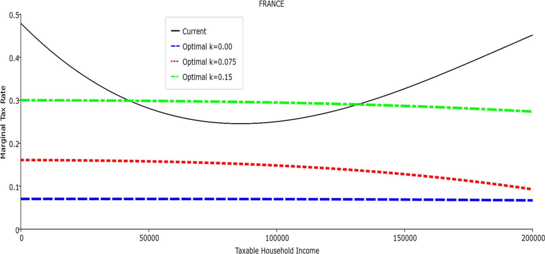
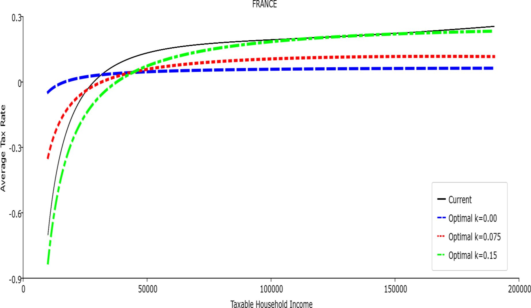
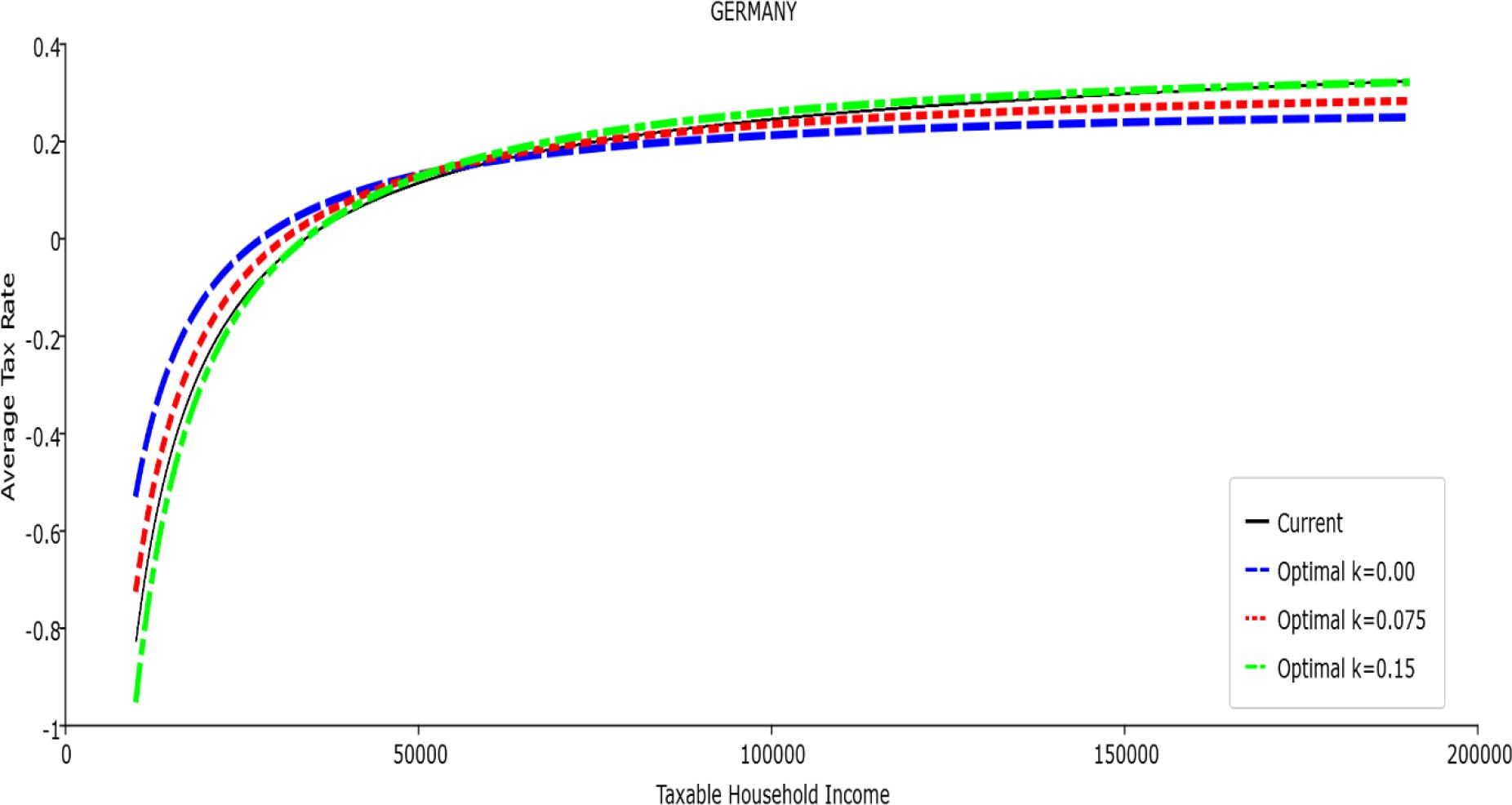
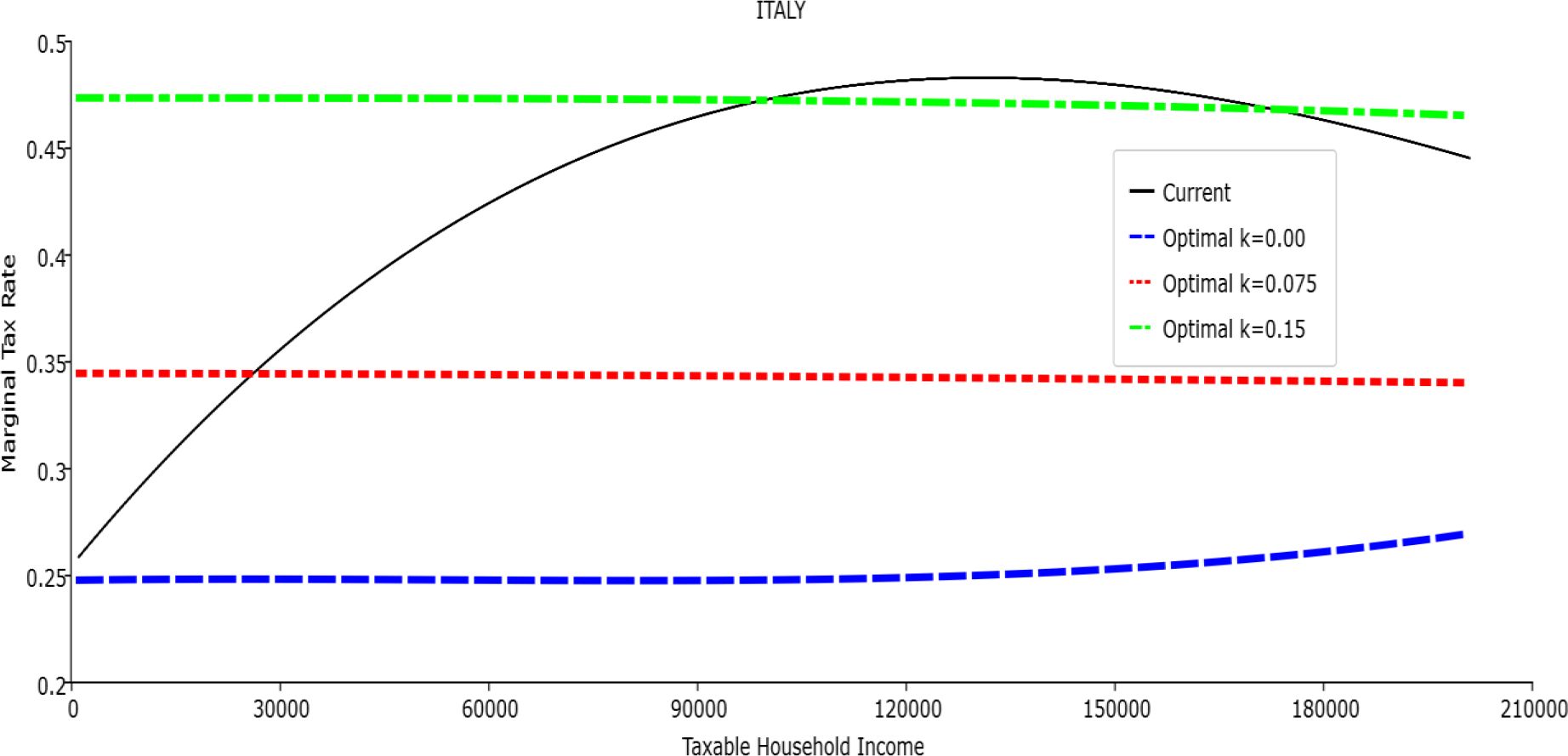
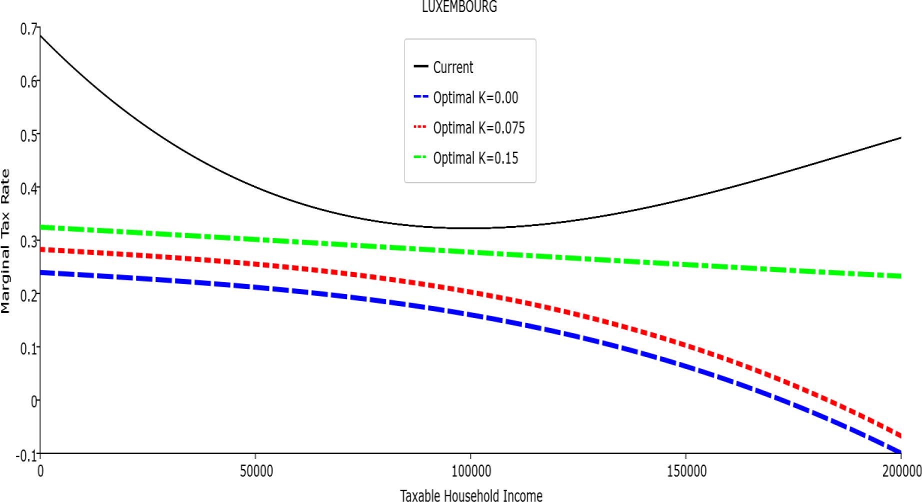
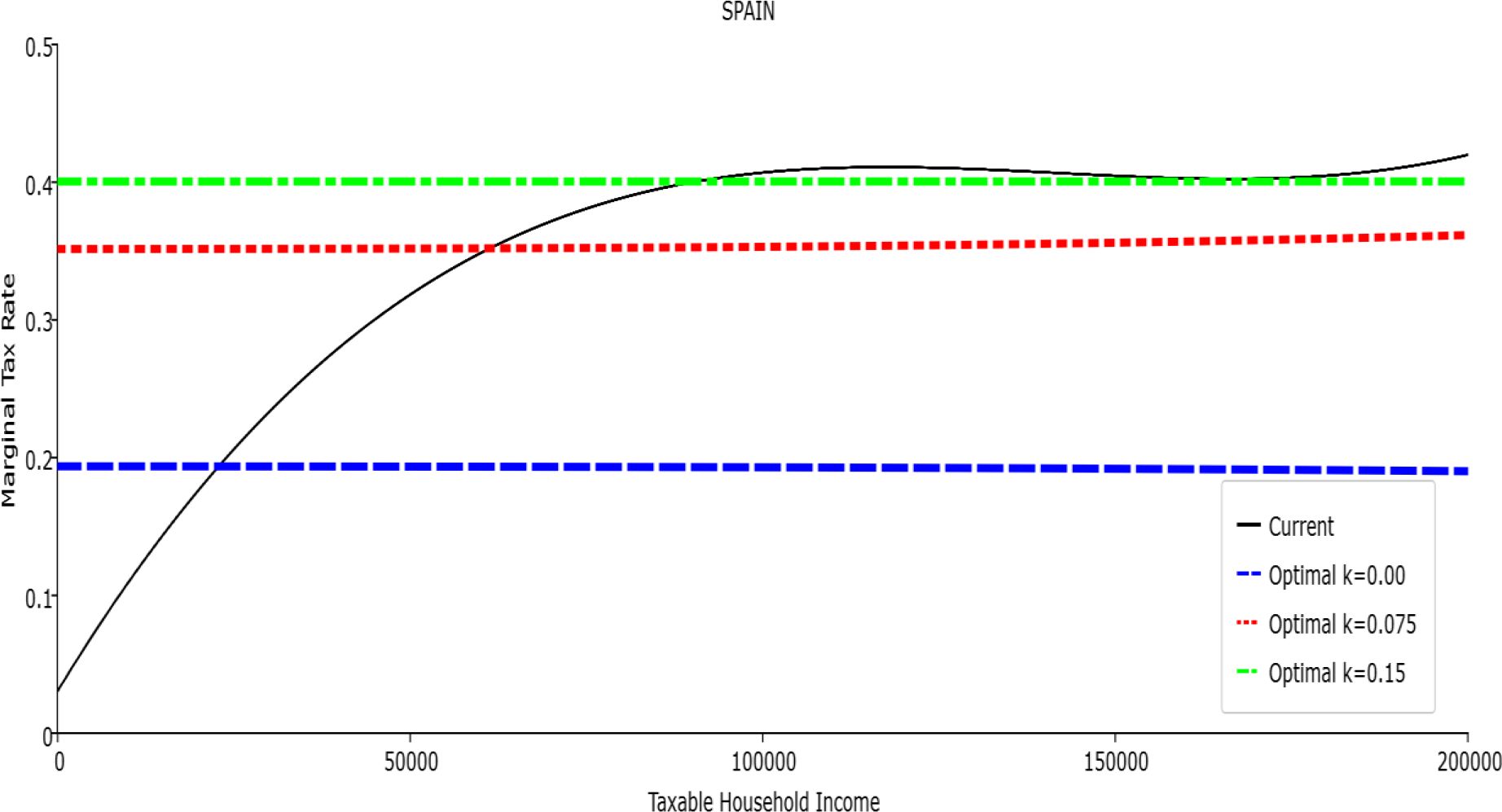
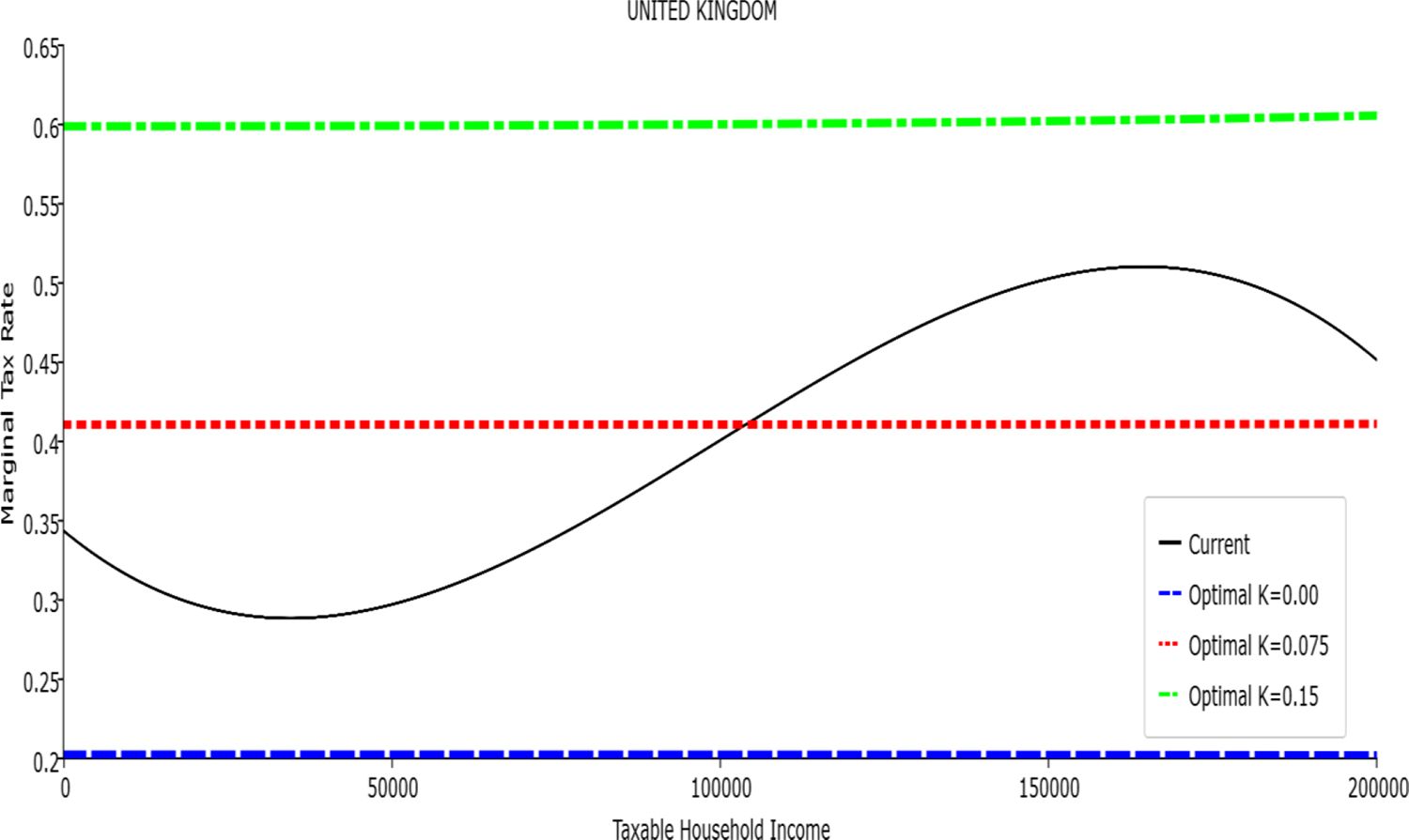
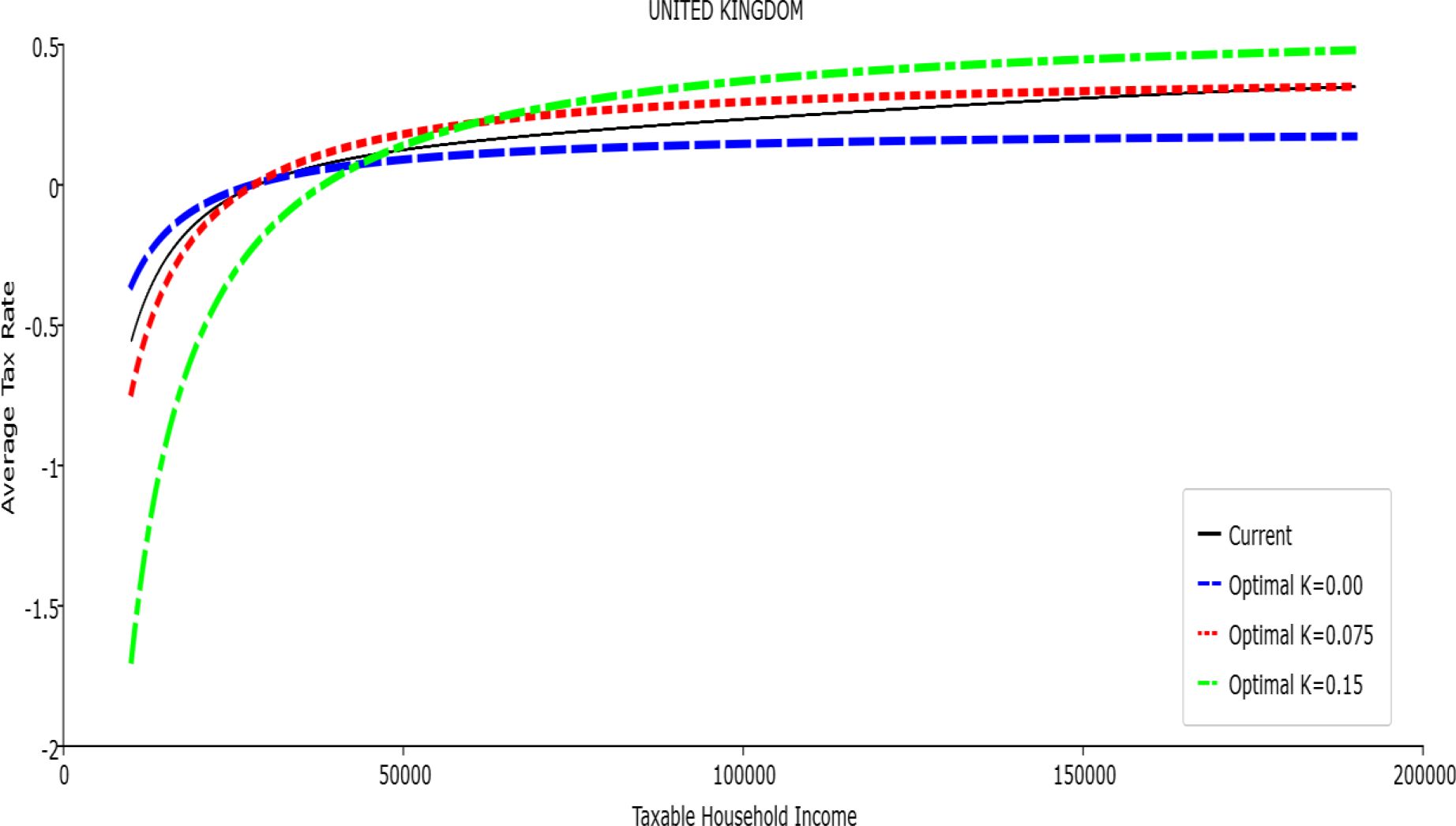
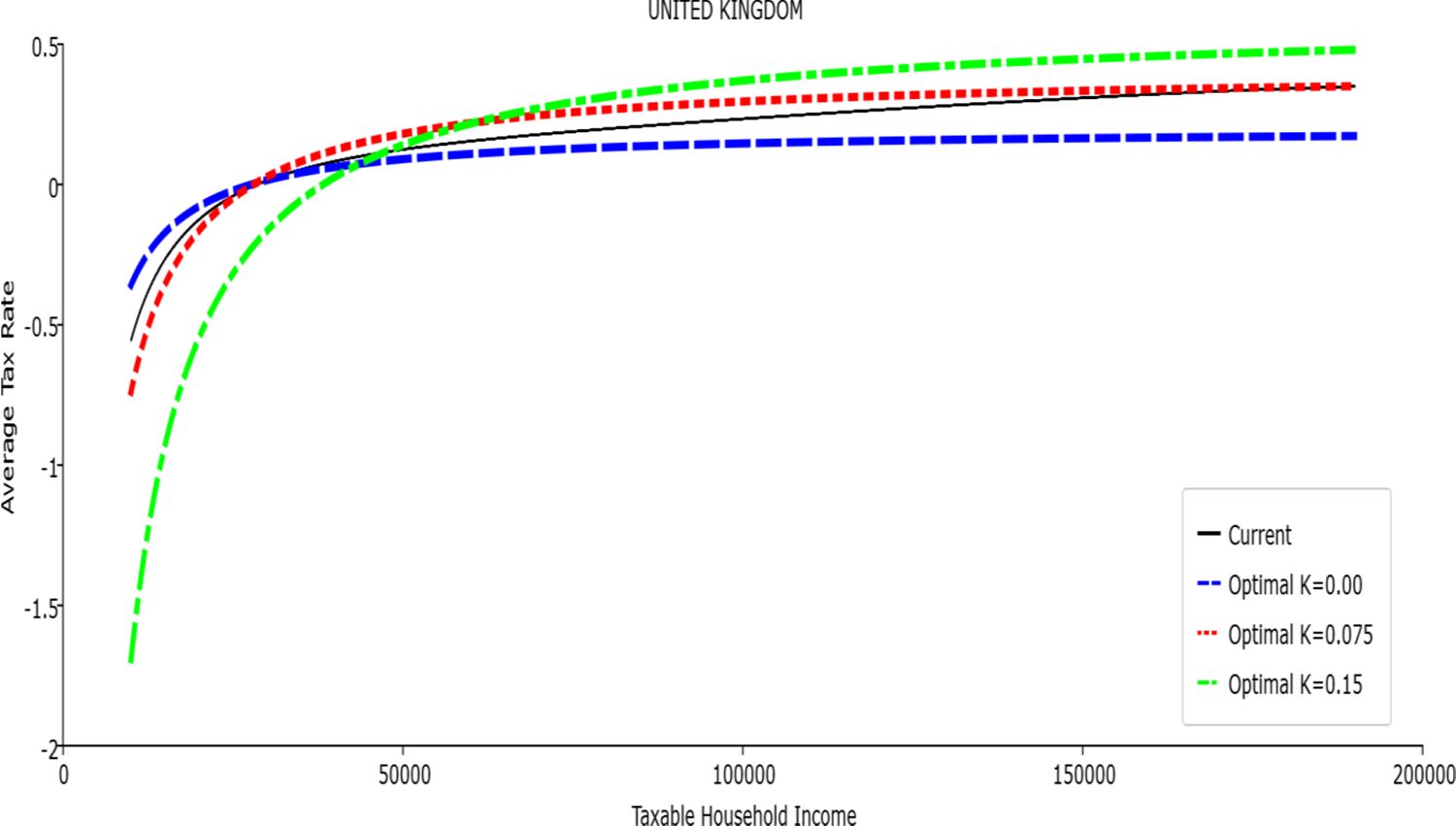
Table 1 reports the parameters of the polynomial optimal TTRs and the polynomial approximation to the current TTRs. The polynomial approximations to the current TTR are just shown to provide a simple comparison between the optimal rules and the current ones: all the other results (welfare and economic effects) relative to the current TTRs are actually obtained with the real current TTRs, not the approximated ones. The welfare gains of the optimal TTRs and the “winners” with respect to the current TTR are reported in Table 2. Figures 1–12 show the marginal tax rates (MRTs) and the average tax rates (ATRs) of the optimal polynomial TTRs and of the approximated current TTRs. Figures 13–20 illustrate other aspects of the welfare and economic effects of the optimal rules.
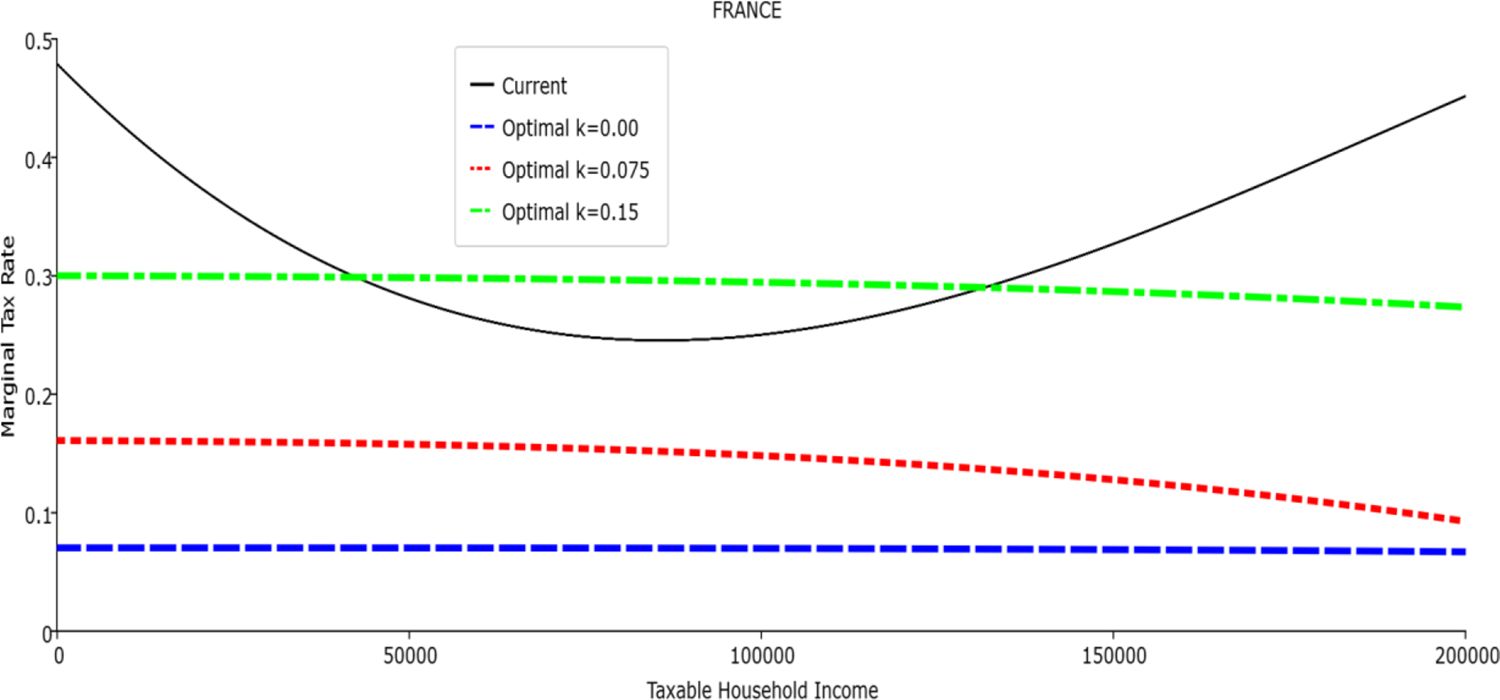
Marginal Tax Rate vs. Taxable Income. France

Average Tax Rate vs. Taxable Income. France

Marginal Tax Rate vs. Taxable Income. Germany

Average Tax Rate vs. Taxable Income. Germany
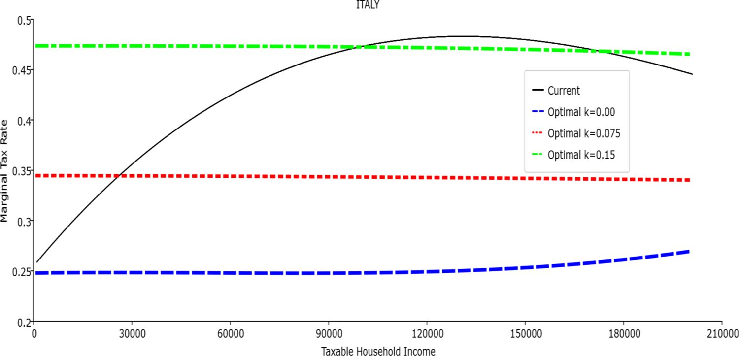
Marginal Tax Rate vs. Taxable Income. Italy

Average Tax Rate vs. Taxable Income. Italy

Marginal Tax Rate vs. Taxable Income. Luxembourg

Average Tax Rate vs. Taxable Income. Luxembourg
Marginal Tax Rate vs. Taxable Income. Spain
Average Tax Rate vs. Taxable Income. Spain
Marginal Tax Rate vs. Taxable Income. United Kingdom
Average Tax Rate vs. Taxable Income. United Kingdom

France: %change of CMU by demographic group and decile, k = 0.075.

France: %change of CMU by demographic group and decile, k = 0.075.

Italy: %change of CMU by demographic group and decile, k = 0.075.

Luxembourg: %change of CMU by demographic group and decile, k = 0.075.

Spain: %change of CMU b.y demographic group and decile, k =0.075

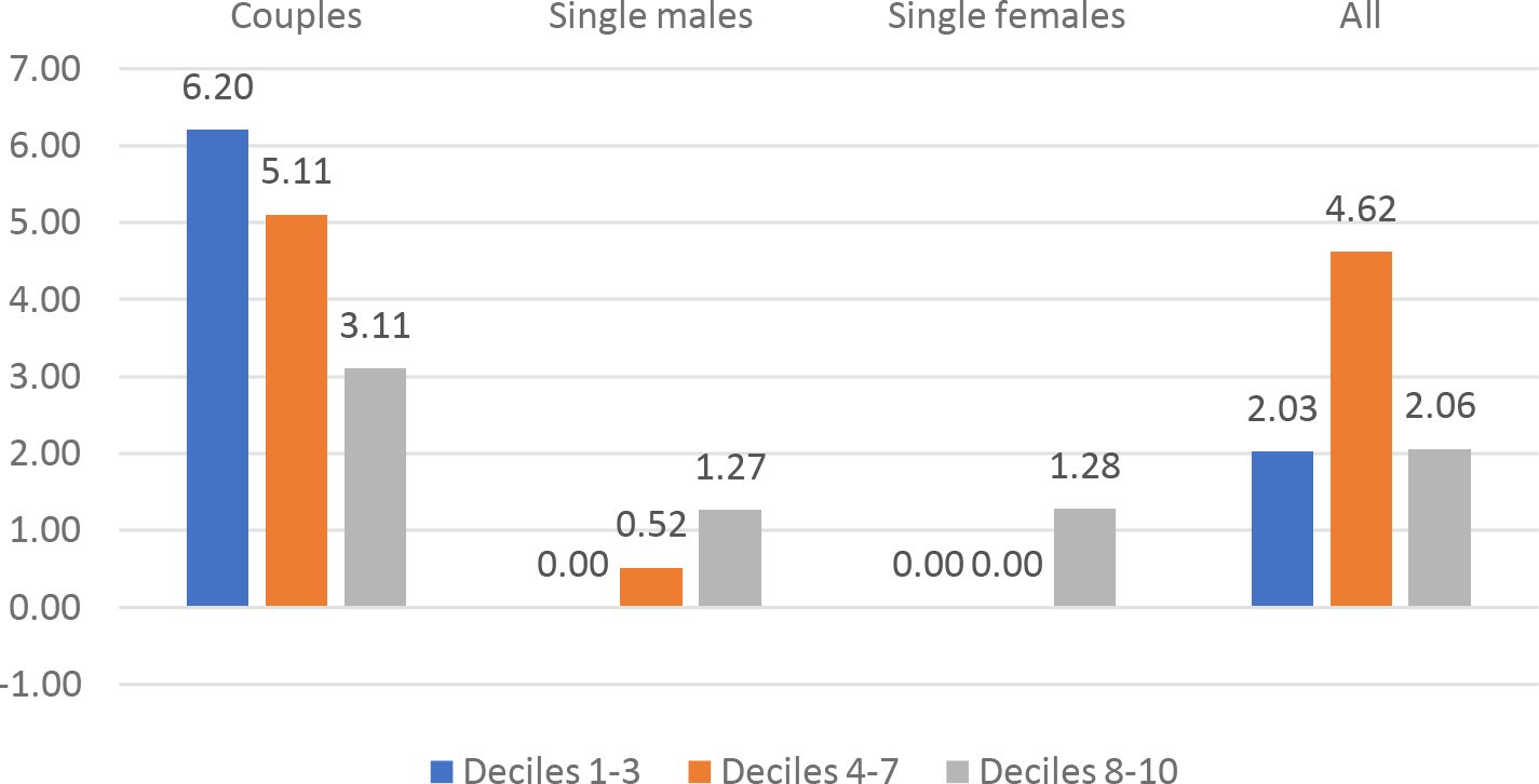
The UK: %change of CMU by demographic group and decile, k = 0.075.
%change of disposable income w.r.t. current values by country and Kolm’s k.
Povery Gap Index by country and Optimal TTR (indexed by Kolm’s k).
Welfare Gains and Welfare Winners
| k = .00 | k = .05 | k= .075 | k = .10 | k =.125 | k = .15 | ||
|---|---|---|---|---|---|---|---|
| France | Social Welfare Gain | 159.23 | 89.63 | 53.17 | 16.37 | -8.6 | -45.47 |
| Equality Gain | 0 | -20.31 | -20.64 | -12.4 | -1.86 | 20.3 | |
| Efficiency Gain | 159.23 | 109.94 | 73.81 | 28.77 | -6.64 | -65.77 | |
| %Winners: All | 67 | 67 | 66 | 65 | 64 | 61 | |
| %Winners: Couples | 66 | 66 | 65 | 64 | 62 | 57 | |
| %Winners: Single Males | 84 | 80 | 76 | 71 | 66 | 62 | |
| %Winners: Single Females | 51 | 55 | 57 | 61 | 66 | 72 | |
| Germany | Social Welfare Gain | -7.48 | -5.00 | 41.05 | 71.39 | 87.65 | 155.27 |
| Equality Gain | 0 | -2.02 | 8.51 | 23.68 | 39.94 | 78.61 | |
| Efficiency Gain | -7.48 | -2.98 | 32.54 | 47.71 | 47.71 | 76.66 | |
| %Winners: All | 46 | 44 | 46 | 46 | 46 | 49 | |
| %Winners: Couples | 41 | 41 | 41 | 41 | 41 | 41 | |
| %Winners: Single M | 37 | 38 | 38 | 40 | 40 | 41 | |
| %Winners: Single F | 55 | 56 | 62 | 63 | 63 | 71 | |
| Italy | Social Welfare Gain | 72.9 | 45.93 | 28.4 | 18.64 | -1.35 | -18.54 |
| Equality Gain | 0 | -3 | -3.06 | -2.97 | 0.13 | 3.16 | |
| Efficiency Gain | 72.9 | 48.93 | 31.46 | 21.61 | -1.48 | -21.70 | |
| %Winners | 56 | 58 | 58 | 57 | 53 | 52 | |
| %Winners: Couples | 51 | 49 | 44 | 42 | 38 | 36 | |
| %Winners: Single M | 59 | 66 | 69 | 70 | 63 | 61 | |
| %Winners: Single F | 58 | 63 | 65 | 65 | 64 | 63 | |
| Luxembourg | Social Welfare Gain | 2.06 | -35.63 | -68.35 | -62.63 | -67.54 | -66.94 |
| Equality Gain | 0 | -41.82 | -43.04 | -46.45 | -40.26 | -27.94 | |
| Efficiency Gain | 2.06 | 6.19 | -25.31 | -16.18 | -27.28 | -39.00 | |
| %Winners | 45 | 48 | 46 | 48 | 49 | 51 | |
| %Winners: Couples | 54 | 59 | 54 | 58 | 59 | 61 | |
| %Winners: Single M | 31 | 32 | 31 | 30 | 30 | 30 | |
| %Winners: Single F | 44 | 47 | 48 | 50 | 52 | 56 | |
| Spain | Social Welfare Gain | -16.99 | -13.87 | 10.65 | 13.83 | 21.35 | 27.17 |
| Equality Gain | 0 | 2.17 | 13.88 | 20.25 | 25.47 | 30.29 | |
| Efficiency Gain | -16.99 | -16.04 | -3.23 | -6.42 | -4.12 | -3.12 | |
| %Winners | 73 | 73 | 67 | 63 | 63 | 63 | |
| %Winners: Couples | 75 | 75 | 63 | 56 | 56 | 55 | |
| %Winners: Single M | 70 | 70 | 72 | 70 | 70 | 70 | |
| %Winners: Single F | 70 | 70 | 73 | 73 | 74 | 74 | |
| United Kingdom | Social Welfare Gain | -18.37 | 37.42 | 37.81 | 48.34 | 65.19 | 77.19 |
| Equality Gain | 0 | 0.81 | 1.14 | 1.24 | 0.64 | -0.17 | |
| Efficiency Gain | -18.37 | 36.61 | 36.67 | 47.10 | 64.55 | 77.36 | |
| %Winners: All | 42 | 76 | 77 | 79 | 81 | 82 | |
| %Winners: Couples | 23 | 79 | 82 | 84 | 88 | 90 | |
| %Winners: Single M | 57 | 64 | 64 | 65 | 66 | 68 | |
| %Winners: Single F | 64 | 82 | 83 | 83 | 83 | 82 |
The optimal TTRs
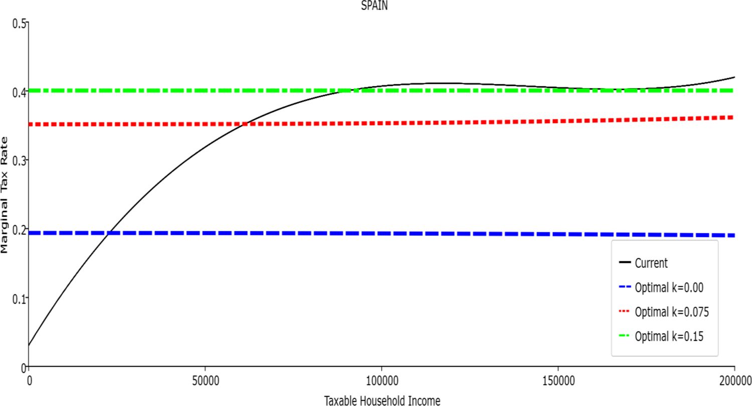
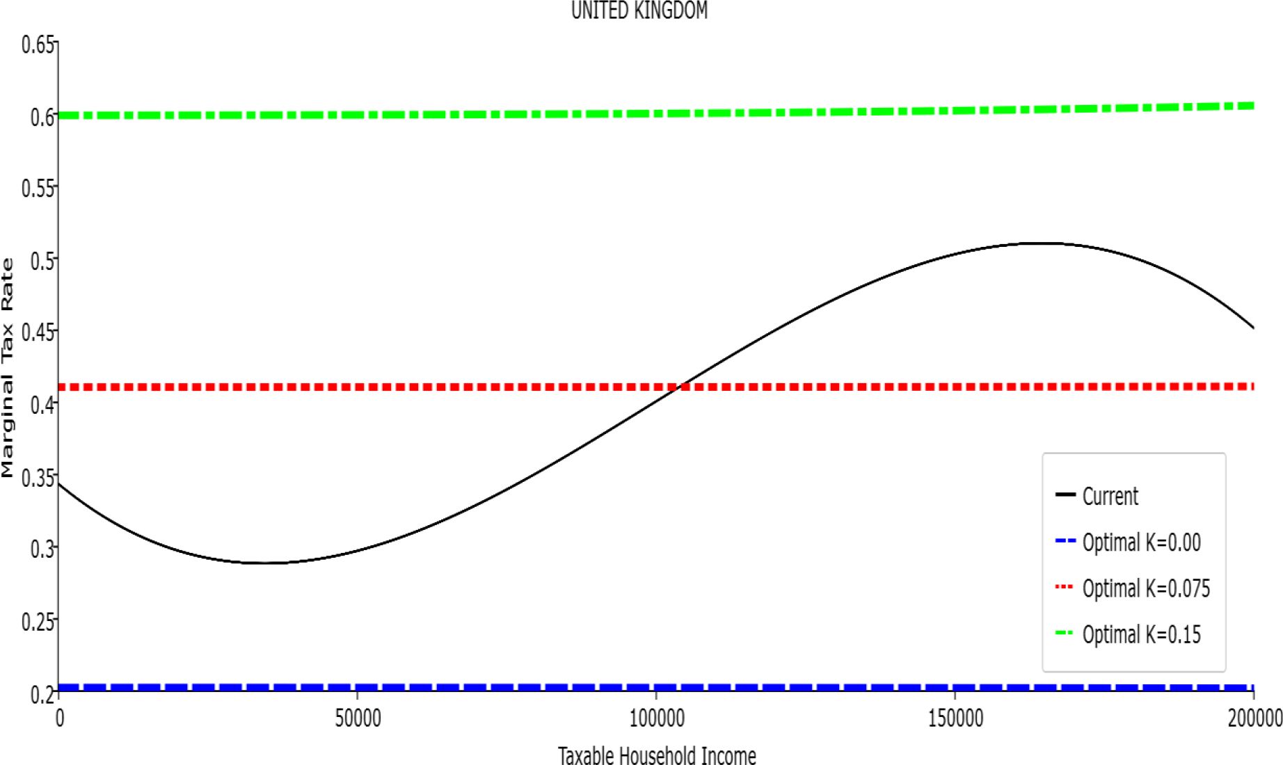
In all the countries, is always positive and the shape of the optimal TTRs is dominated by τ1, while the other parameters are very small and might exert some influence only at large taxable incomes (e.g. above 150000 euro a year). As a consequence, the optimal TTRs are very close to a FT equal to 1-τ1 plus a UBI (or equivalently a NIT). In contrast, in all the countries, the polynomial approximation to the current TTR features important non-linearities. Parameter is the monthly universal basic income (or guaranteed minimum income according to the NIT interpretation) for a one-person household. For a N-person household it must be multiplied by N1/2. Notice that the value of the approximated current TTR is not strictly comparable to the optimized value of , since the latter is a universal and unconditional transfer to be received with certainty, while the former is an expected value across the population of various - mostly means-tested, contingent and categorical - transfers. It makes sense, however, to interpret as a measure of the expected current expenditure in income support policies from the view-point of the public budget constraint. In this perspective – without implying direct policy prescriptions – the current policies appear to be more or less cost-effective than those indicated by the optimized rules. In France and Luxembourg, the current income support policies appear to be “too costly”: a less expensive UBI would attain a higher Social Welfare (for k < 0.125 in France and for k < 0.05 in Luxembourg). The opposite holds in Germany and Italy (for k > 0.05), Spain (for all considered value of k) and the United Kingdom (for k 0.05). The main features of the optimal polynomial TTRs are also illustrated in the Figures 1–12. The effects of the other parameters on the shape of the TTRs are illustrated by the Figures 1–12, which respectively represent MTR and ATR as functions the household total taxable income.15 The graphs are built under the assumption that the optimal TTRs are implemented by paying the UBI and then applying the tax rates to the taxable income. Note the almost flat MTR hold whatever the value of the inequality aversion parameter k. The implication is that, within the TTR class considered, a certain degree of progressivity is more efficiently attained by a UBI or a NIT with non-distortive MTRs rather than by increasing and distortive MTRs. We also represent the MTR of the polynomial approximation to the current TTR. Note that it does not correspond to official values of the current MTRs. It measures the change – averaged across the households – in total household taxes when total household taxable income increases by one euro. It shows striking differences both between the countries and with respect to the optimal polynomial TTRs. The current systems in France and Luxembourg appear to envisage relatively generous income support policies at low or zero income followed by very high implicit marginal benefit reduction rates. The optimal rules suggest less expensive (although universal and unconditional) income support and a longer and smoother phase-out. Germany envisages an expensive current income support policies and yet a slowly increasing MTR on low incomes. In Italy and Spain, the current MTRs are first steeply increasing up to taxable incomes around 100,000 and then decreasing.
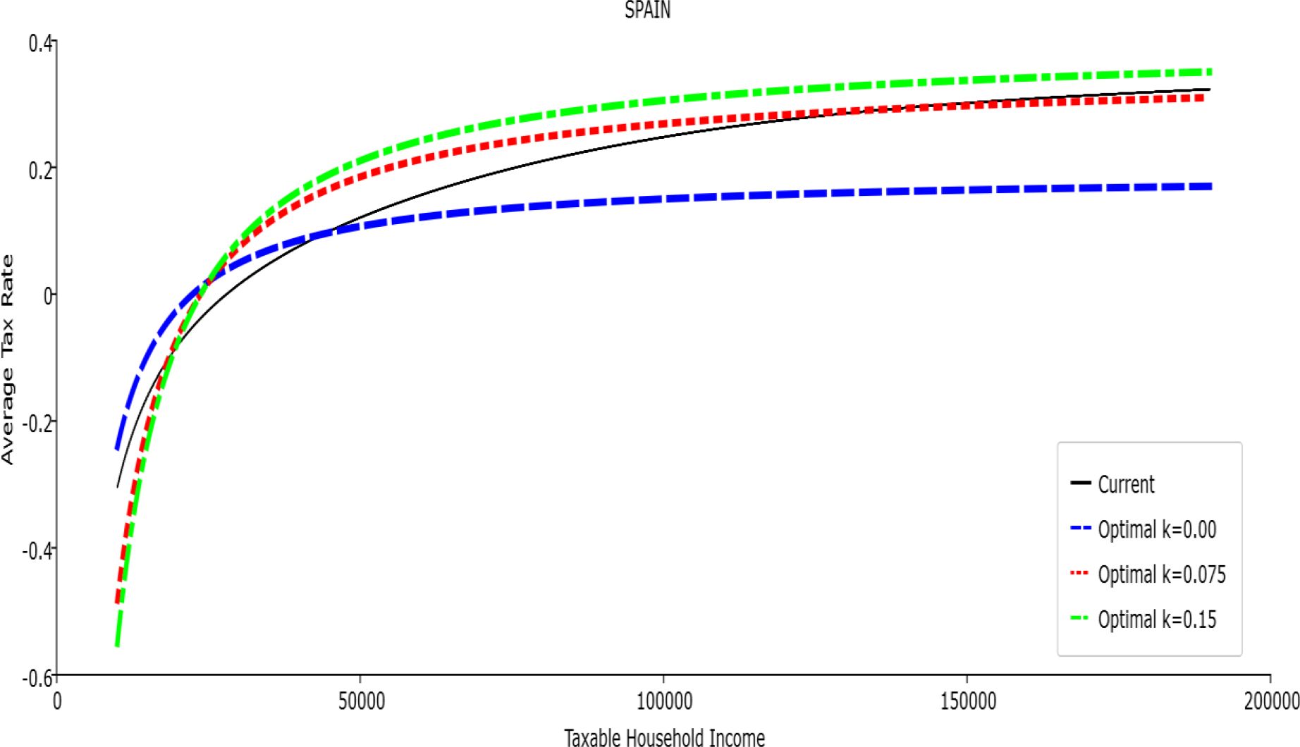
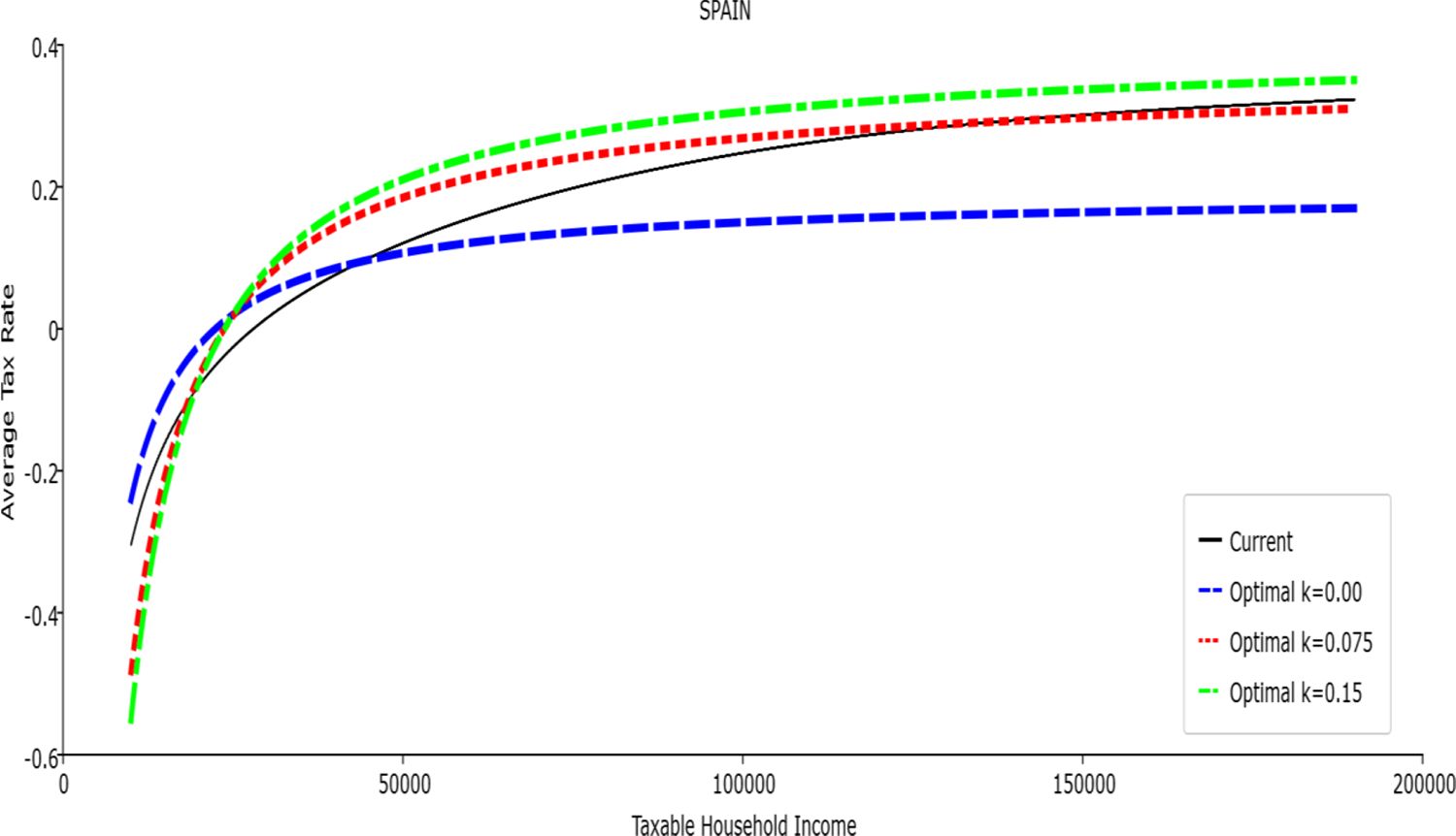
Given that the optimal MTRs are very close to a constant, the ATRs (Figures 1–12) are useful to show the level and type of progressivity implied by the various TTRs in the different countries.16 If the Social Welfare criterion ignores inequality effects (i.e. k = 0.00), in all the countries the optimal TTR – as compared to the current TTR – is more progressive on low levels of taxable income and less progressive on middle or high taxable incomes. The opposite happens with k=0.15. This holds in general, although in Luxembourg and Germany the ATRs are very close for different values of k, i.e. the ATR behaves approximately in the same way whatever the value of k. For k = 0.075, the optimal ATR is closer to the current one, but less progressive on middle and high incomes in France and Italy.
Welfare effects
The Social Welfare Gains, the Equality Gains and the Efficiency Gains due to the optimal polynomial TTRs (with respect to the current TTFs) by country and Kolm’s k are reported in Table 2. For most countries and most values of k, the optimal polynomial TTR is social welfare superior to the current TTR. This result holds in France and Italy for k < 0.15, in Luxembourg for k < 0.05, in Germany and Spain for k 0.075 and in the United Kingdom for k 0.05. What happens is that the polynomial optimal TTRs are mainly disequalizing in France, Italy and Luxembourg but equalizing (for a majority of k values) in Spain and in the United Kingdom. As consequence, higher values of k – i.e. higher costs of inequality – tend to overcome the efficiency effect in the former group of countries and strengthen it in the latter one. These results are also due to the efficiency gain, which decreases with k in the first group of countries while it increases in the second one.
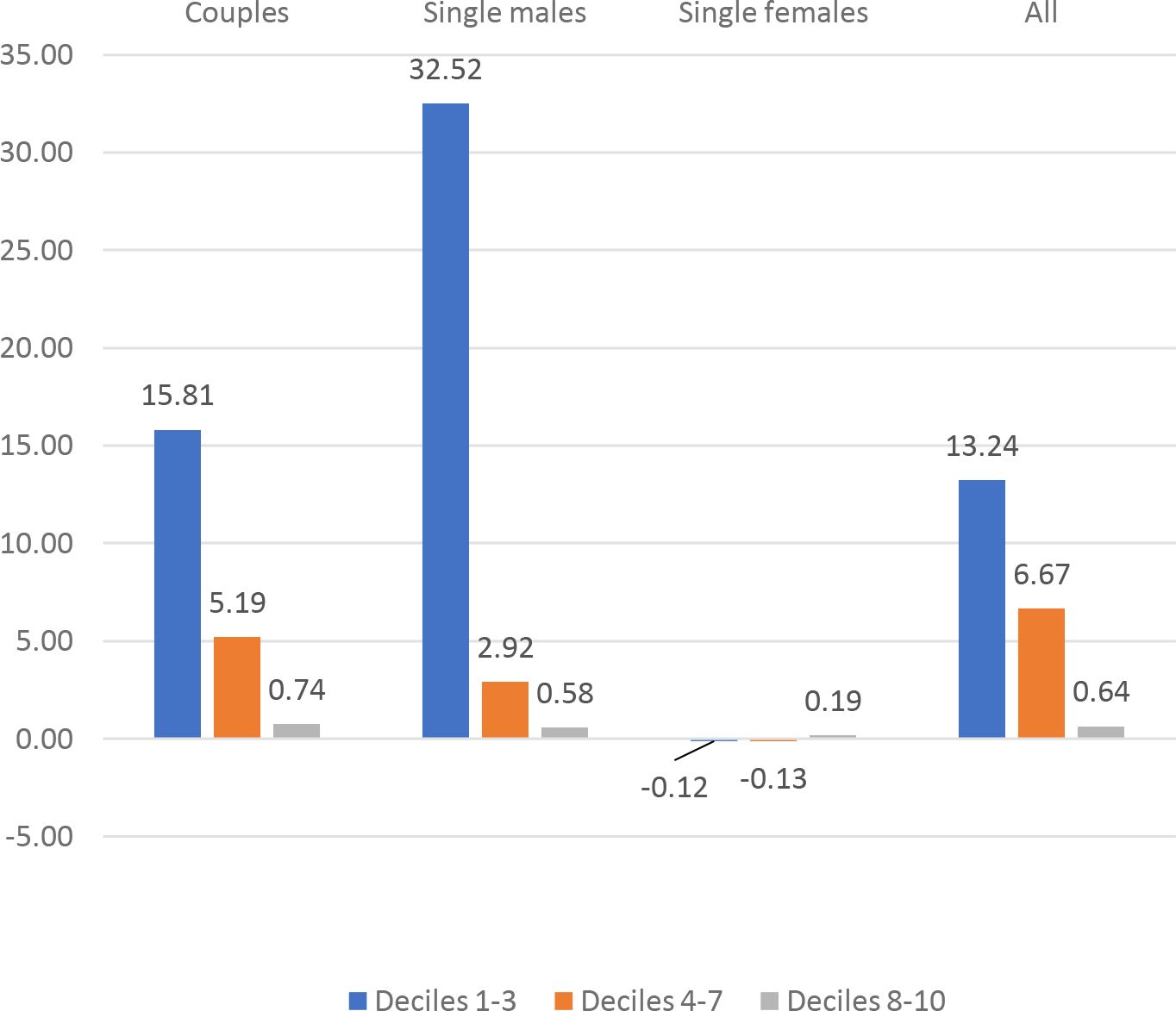
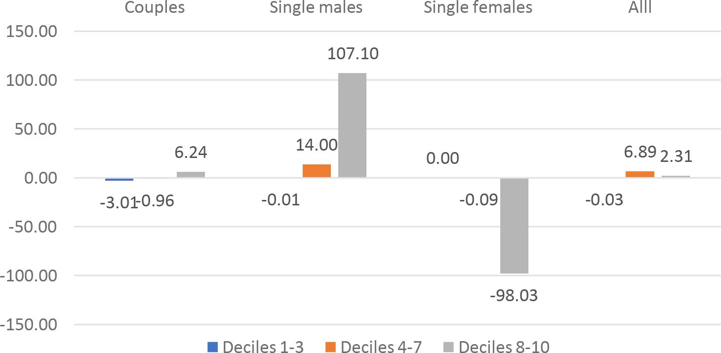
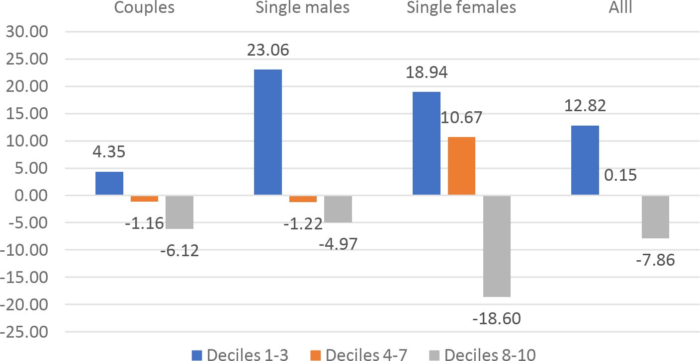
Besides the overall Social Welfare effects, we can identify specific welfare effects for different demographic groups. We have computed the CMU (Section 4.3) of couples, single males and single females under the current TTR and under the optimal TTRs for k = .075.17 show the average CMU gains for the different demographic groups, by decile (1-3, 4-7, 8-10) of current CMU distribution. The graphs show an extreme heterogeneity across countries, demographic groups and deciles. Depending on the country, some groups and/or some deciles are penalized by the optimal polynomial TTRs. System like UBI+FT or NIT+FT are typically expected to penalize middle income deciles. In our results this seems to be the case except for France and Germany.18
Table 2 shows also the percentages of households who “win” under the optimal polynomial TTRs by country, type of household (couple, single male, single female) and Kolm’s k. A household is classified as a winner if its CMU under the optimal polynomial TTR is larger than its CMU under the current TTR. The information conveyed is ordinal and therefore is different from the cardinal information conveyed by. The percentage of winners can be interpreted as an estimate of the support that a given TTR would receive in a referendum. Also the results on winners confirm the heterogeneity of the effects of the optimal TTRs, which receive more support by single females in Germany, by single female and single males in Italy and by couples in Luxembourg. By contrast, in France, Spain and the U.K., the optimal TTRs receive a rather uniform support by the different type of households.
Economic effects
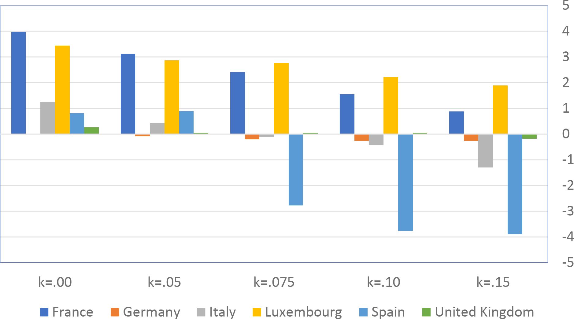
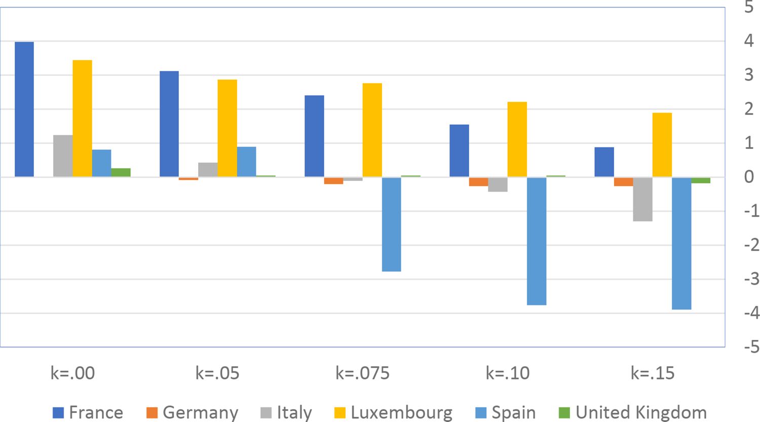
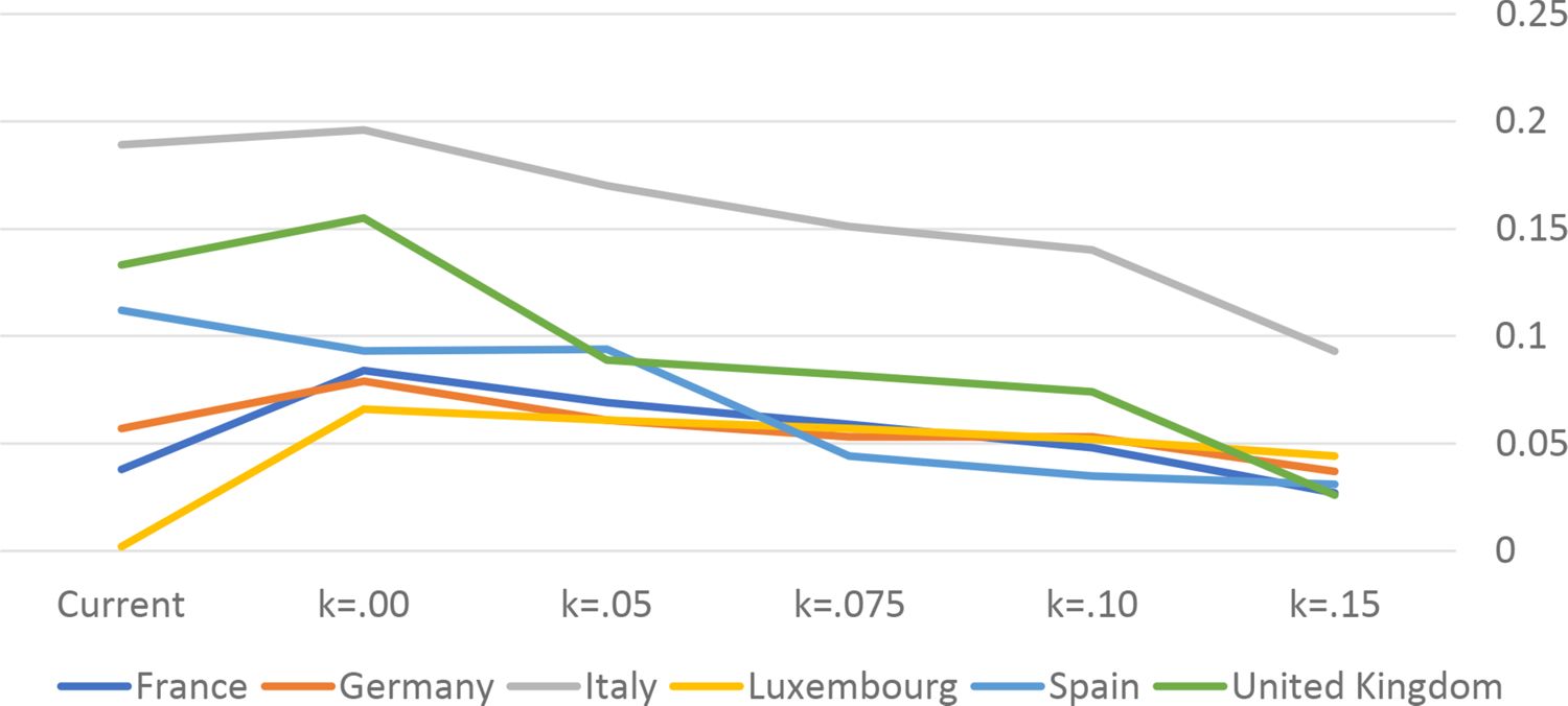
Figure 19 and Figure 20 represent the percentage change in disposable income and the Poverty Gap Index respectively, by country and Kolm’s k. The two graphs illustrate a dimension of the efficiency-equality trade-off. Disposable income increases as long as , with the exception of Germany. With k > 0.05 it keeps increasing in France and Luxembourg, while it decreases in Germany, Italy and the United Kingdom. The aggregate effects on labour supply (not reported) are small and consistent with the dynamics of disposable income. The Poverty Gap Index increases when the economy adopt the polynomial optimal TTR with k = 0, then it decreases with increasing inequality aversion k.
The “primitives” and the optimal TTRs
Table 3 shows illustrative results obtained by inferring a general rule that links the “primitives” to the optimal TTRs, i.e. it presents the results of the analysis explained in Section 4.5. We have well-defined results on UBI (τ0): all the coefficients are significant at standard levels . Kolm’s k, Productivity and Elasticity (both extensive and intensive) elasticities favour a higher UBI. A stricter Budget require a lower UBI. Among the above results, the surprising one is the effect of elasticities. A possible explanation is that UBI, as compared to means-tested policies does not suffer from poverty-traps, therefore its relative advantage is greater the more elastic is household behaviour. Kolm’s k and Extensive elasticity respectively favour a lower and a higher Leading Tax rate: the former result, taken together with k’s effect on UBI, seems to mean that more egalitarian social preferences favour a higher UBI rather than higher taxes; the latter result might mean that less distortions are better achieved with UBI than with lower taxes. Let us imagine we want to propose a common TTR to all the countries, based on the averages of the “primitives”. Let us also suppose that social preferences are such that k = 0.075. Then the UBI (or equivalently the guaranteed minimum income in a NIT rule) and the leading tax rate of the common polynomial optimal TTR would be 456 monthly euros (for one-person household) and 29.8% respectively. It is close to the optimal TTR in Germany for k = 0.05.
“Primitives” of the economy and characteristics of the optimal polynomial TTRs
| UBI | Leading Tax Rate | |
|---|---|---|
| Constant | 357.28 2.14 | -5.04 -0.3 |
| Kolm’s k | 25.44 14.01 | 1.40 9.95 |
| Productivity | 0.22 11.29 | 0.002 1.48 |
| Extensive Elasticity | 117.35 3.05 | 9.90 3.31 |
| Intensive Elasticity | 253.55 8.44 | 1.46 0.62 |
| Budget | -0.25 -8.08 | 0.002 -0.85 |
| R2 | 0.83 | 0.88 |
| Standard error of the estimate | 53.69 | 0.04 |
-
t-values in italics below the estimates.
-
Bold estimates are significant at standard levels.
Concluding remarks
Two main approaches to empirical optimal income taxation have been used so far in the literature: the analytical and the computational approach.
In this paper we develop a version of the computational approach that combines microeconometric modelling, microsimulation, numerical optimization and social welfare evaluation in a consistent way.
We consider the class of 4th degree polynomial TTRs, i.e. a generic rule that represents total household disposable income as a 4th degree polynomial function plus a constant. We adopt the Kolm’s social welfare function. A specific TTR is defined by the parameter vector containing the four coefficients of the polynomial and the constant. We identify optimal TTRs for different degrees of social inequality aversion and compare them to the current rules in six European countries.
For most countries and most values of the inequality aversion parameter, the optimal polynomial rules provide a higher social welfare than the current ones. The class of TTRs considered as candidates for welfare optimality, although flexible, is extremely simple. It is applied to the total taxable household income, irrespective of the source of income. It does not depend on household’s socio-economic characteristics, with the exception that the number of household members that affects the basic income transfer. It is of course quite possible that we might do better by taking households’ heterogeneity into account when designing the optimal TTR. However, finely categorized, targeted and means-tested TTRs bear administration and political costs (complex forms to file out, monitoring, political manipulation, lack of transparency, conflict resolution etc.) that are certainly less important or even not existent in simple and universalistic TTRs.
The results suggest some common features in all the countries. The optimal polynomial TTRs are very close to a (almost) FT plus UBI or equivalently plus NIT. The profiles of the MTRs are pretty similar in different countries and definitely flatter than under the current TTRs. This results hold for all the countries and all the values of the inequality aversion k, despite the fact that the polynomial TTR class is flexible and the heterogeneous responses allowed by the microeconometric model might induce very different shapes of the optimal TTRs. These results confirm those of Islam and Colombino (2018). This is remarkable, since Islam and Colombino (2018) only compare the NIT+FT rule to the current TTR, while the polynomial class considered in this paper is very flexible and compatible with many different shapes of the TTR. The social welfare gains due to the optimal polynomial TTRs are admittedly small. However, the results show that extremely simple universalistic TTRs (five parameters) can at least match the performance of the very complex current TTRs (dozens or even hundreds of parameters).
The TTRs that come out as optimal in our exercise are far from the current ones. However, they are not outside the choice set considered by the policy debate. The FT has been implemented in many Eastern European countries and it has been proposed by many economists.19 UBI is receiving an increasing interest.20 The “package” UBI+FT has been studied with a micro-macro model by Magnani and Piccoli (2020). A recent theoretical and empirical (stochastic dynamic macroeconomic model) analysis by Ferriere et al. (2021) gives support to the conclusion that a TTR close to UBI+FT might be optimal.
Despite the above common features, we can see large differences between the levels of UBI and the values of the MTRs under the optimal polynomial TTRs in the different countries. They depend indeed on various characteristics of the population and the economic environment.
The differences of optimal TTRs in different countries, therefore, call for a further step. An explanation of these differences among countries requires to identify a general relationship between the basic (“primitive”) characteristics of the economy and the features of the optimal TTRs. Actually, this is the direct result of the analytical solution of optimal taxation. We can come close to a similar result by replacing the analytical solution with microsimulation and numerical optimization. Even with a limited number of countries, we exemplify the procedure that can be used to identify the effects of “primitives” (Kolm’s k, Productivity, Extensive and Intensive Elasticities, Public budget constraint) upon two characteristics of the optimal TTRs (UBI and Leading tax rate). A notable and surprising results is that elasticity favours a preference for UBI while it has a little effect on taxes. Also, more egalitarian social preferences favour a higher UBI rather than higher taxes. Overall, it seems that that less distortions and more equality are better achieved through UBI rather than through taxes.
As a final comment, it must be noted that the level of abstraction of the computational exercise illustrated in this paper is close to the one that characterizes the analytical approach. A similar level of abstraction holds by construction for any exercise in empirical optimal taxation, but in the case of our exercise is also due to an explicit choice (i.e. choosing a simple – though flexible – and universalistic class of TTRs). Moreover, we claim that the computational approach might have better opportunities to reflect realistic features of the economy (due to the use of a flexible microeconometric model). Although the results of optimal taxation exercises cannot be taken as immediate recipes for reform, yet they indicate reform directions that might deserve further detailed investigations, which can then account – to a certain extent – for some of the features and constraints that presumably led the current real TTR. The challenge being to identify policy flaws that can be fixed by reforms.21
Footnotes
1.
It is interesting to see that the modern dynamic general equilibrium literature (e.g. Ferriere et al., 2021; Heathcote and Tsujiyama, 2021) appears to prefer the “Ramsey approach” (parametric tax rule) rather than the “Mirlees approach” (non-parametric tax rule).
2.
See for example: Atkinson (1996), Colombino (2015), Colombino and Islam (2018), Colombino and Narazani (2013), Gentilini et al. (2020), Ghatak and Jaravel (2020), Ghatak and Maniquet (2019), Grimalda et al. (2020), Islam and Colombino (2018), Magnani and Piccoli (2020), Moene and Ray (2016), Standing (2011; 2015), Van Parijs and Vanderborght (2017).
3.
Of course one might adopt different evaluation criteria, such as the effects on employment, poverty etc. We adopt a social welfare criterion but we will also report and discuss results on other indices that might be policy-relevant.
4.
Given the limited number of countries, we are only able to present an illustrative example of the identification of the “mapping” from “primitives” to optimal TTrs.
5.
The acronym RURO (= Random Utility-Random Opportunity) is proposed by Aaberge and Colombino (2014).
6.
The dataset for France is the Statistics on Resources and Living Conditions (SRCV) survey, the France part of the EU-SILC survey produced by Public Statistics Data Archives (ADISP).
7.
EUROMOD is a large-scale pan-European tax-benefit static micro-simulation engine (e.g. Sutherland and Figari, 2012). It covers the tax-benefit schemes of the majority of European countries and allows computation of predicted household disposable income, on the basis of gross earnings, employment and other household characteristics.
8.
In all the optimal TTRs we obtain τ0 > 0. The equivalence of a universal basic income and a universal negative income tax with guaranteed minimum income can be easily seen in the flat tax case, although it carries over to non-flat taxes. See for example Hoynes and Rothstein (2019).
9.
In this paper we identify optimal TTRs for six value of k: 0.0, 0.05, 0.075, 0.10, 0.125, and 0.15. It can be shown (Islam and Colombino, 2018) that the corresponding values of the popular Atkinson’s parameter of inequality aversion are approximately 0.000, 0.114, 0.180, 0.252, 0.333 and 0.424.
10.
Kolm’s Inequality Index is an absolute index, meaning that it is invariant with respect to translations (i.e. adding a constant to every μi). Absolute indices are less popular than relative indices (e.g. Gini’s or Atkinson’s), although there is no strict logical or economic motivation for preferring one to the other. Atkinson and Brandolini (2010) provide a discussion of relative indices, absolute indices and intermediate cases. Depending on the specific applcation, there might be a motivation of computational convenience for choosing one or another type of index. Blundell and Shephard (2012) adopt a social welfare index which turns out to be very close to Kolm’s index. Their main motivation for their index seems to be computational, since it handles negative numbers (random utility levels). Our motivation is analogous.
11.
In order to locate a global maximum, we partition the parameter space and try different starting values.
12.
It might be argued that “primitives” 2 – 5, are not really primitives, since they are also determined by the current TTRs. This is true, but it is not really relevant. We interpret our analysis as conditional upon the current economy.
13.
With a suitable – larger – sample of countries, one could adopt a better method. For example, the identification of the optimal TTR in a country could be modelled as a conditional logit, where the decision maker is the “social planner”, the objects of choice are alternative TTRs belonging to the polynomial class and the “primitives” interact with the attributes of the alternative TTRs. Then one could estimate the effects of the “primitives” upon the attributes of the chosen TTR.
14.
The term intensional (as the term extensional at point b) is used in the logical sense. For example, the intensional definition of an object is a specification of the characteristics that permit to identify the object. The extensional definition of an object consists of directly pointing at (or showing) the object.
15.
In Graphs 1 – 12 the current MTRs and ATRs are computed with the polynomial approximation to the true current TTR (see the end of Section 4.2).
16.
A simple index of progressivity is MTR/ATR.
17.
The shape of results is similar for different values of k.
18.
These problems might probably be moderated by a country-specific design of the equivalence scale applied to the basic income.
19.
20.
Among many others: Colombino (2019), Hoynes and Rothstein (2019), Ghatak and Maniquet (2019), Benzell and Ye (2021).
21.
The Mirrlees Review represents a notable example where abstract optimal taxation results – in that case obtained by the Mirrlees-Saez methods – are taken as a basis for formulating specific reform proposal (Mirrlees et al., 2011).
Appendix 1
Maximum likelihood estimates – couples (France)
| Model component | Variable | Coef. | Std. Err. |
|---|---|---|---|
| Opportunity density | δ | ||
| Employee_Man | 0.4761696 | 0.3665576 | |
| Self-employed_Man | 0.2130577 | 0.3805561 | |
| Employee_Woman | -0.3649212 | 0.2853927 | |
| Self-employed_Woman | -1.426779 | 0.3241603 | |
| Part-time_Employee_Man | -0.3805255 | 0.2414433 | |
| Full-time_Employee_Man | 2.83453 | 0.1249029 | |
| Part-time_Self-employed_Man | -1.841048 | 0.324269 | |
| Full-time_Self-employed_Man | 0.2870089 | 0.1540075 | |
| Part-time_Employee_Woman | 0.6361778 | 0.2170085 | |
| Full-time_Employee_Woman | 2.698627 | 0.1676399 | |
| Part-time_Self-employed_Woman | -1.014395 | 0.3149686 | |
| Full-time_Self-employed_Woman | 0.6781008 | 0.2277644 | |
| Income | γ | ||
| Household_Disposable_income | 0.0003342 | 0.0001334 | |
| Hosuhold_Disposable_income squared | 1.61E-08 | 6.75E-09 | |
| Household_size X Household_disposable_income | -0.0000513 | 0.0000175 | |
| Leisure | λ | ||
| Leisure_Male | 0.1256514 | 0.0281893 | |
| Leisure_Man squared | 0.0000173 | 0.0001373 | |
| Leisure_Woman | 0.163189 | 0.0255661 | |
| Leisure_Woman squared | -0.000107 | 0.0001529 | |
| Leisure_Man X Household_disp_income | -7.88E-06 | 1.02E-06 | |
| Leisure_Woman X Household_disp_income | -1.54E-07 | 8.04E-07 | |
| Leisure_Man X Age_Man | -0.0059183 | 0.0011829 | |
| Leisure_Woman X Age_Woman | -0.0085386 | 0.0009848 | |
| Leisure_Man X Age_Man squared | 0.0000742 | 0.0000138 | |
| Leisure_Woman X Age_Woman squared | 0.0001108 | 0.000012 | |
| Leisure_Man X No. Children | -0.0026133 | 0.0017907 | |
| Leisure_Woman X No. Children | 0.0084813 | 0.0015617 | |
| Leisure_Man X No. Children0-6 | 0.0027957 | 0.0025747 | |
| Leisure_Man X No. Children7-10 | 0.006507 | 0.0027523 | |
| Leisure_Woman X No. Children0-6 | 0.006981 | 0.0021144 | |
| Leisure_Woman X No. Children7-10 | 0.0007436 | 0.002288 | |
| Leisure_Woman X Leisure_Man | 0.0001134 | 0.0000948 | |
| N.observations (N. couples*49 alternatives) | 195804 | ||
| N.couples | 3996 | ||
| LR chi2(32) | 15140.15 | ||
| Prob > chi2 | 0 | ||
| Pseudo R2 | 0.4868 | ||
| Log likelihood | -7981.6412 |
Maximum likelihood estimates – singles (France)
| Male | Female | ||||
|---|---|---|---|---|---|
| Model component | Variable | Coef. | Std. Err. | Coef. | Std. Err. |
| Opportunity density | δ | δ | |||
| Employee | 0.199478 | 0.533068 | -1.19744 | 0.470041 | |
| Self_employed | -0.21333 | 0.593638 | -1.68397 | 0.553979 | |
| Part-time_Employee | -0.69588 | 0.393698 | 1.256628 | 0.352174 | |
| Full-time_Employee | 2.213382 | 0.253926 | 2.994315 | 0.267448 | |
| Part-time_Self-employed | -2.70132 | 0.585303 | -1.80785 | 0.627849 | |
| Full-time_Self-employed | -0.28412 | 0.336337 | 0.368914 | 0.377033 | |
| Income | λ | λ | |||
| Disposable income | -0.00012 | 0.00024 | 7.55E-05 | 0.000379 | |
| Disposable income squared | 4.53E-08 | 2.07E-08 | 6.64E-08 | 4.13E-08 | |
| Household size X Disp_income | -5.6E-05 | 4.62E-05 | -6.7E-05 | 6.84E-05 | |
| Leisure | λ | λ | |||
| Leisure | 0.129227 | 0.029882 | 0.15447 | 0.034747 | |
| Leisure2 | -8.1E-05 | 0.000239 | -9.2E-05 | 0.000254 | |
| Leisure X Disposable income | 1.01E-06 | 2.34E-06 | 6.43E-07 | 3.40E-06 | |
| Leisure X Age | -0.00516 | 0.000963 | -0.0075 | 0.001086 | |
| Leisure X Age squared | 6.36E-05 | 1.21E-05 | 0.000092 | 1.34E-05 | |
| Leisure X No. Children | -0.01374 | 0.005121 | 0.006768 | 0.003433 | |
| Leisure X No. Children 0-6 | -0.00814 | 0.019875 | 0.015925 | 0.00544 | |
| Leisure X No. Children 7-10 | 0.011728 | 0.010413 | 0.008727 | 0.004892 | |
| Other | |||||
| N.observations (N. single*7 alternatives) | 9331 | 10465 | |||
| N.single | 1333 | 1495 | |||
| LR chi2(17) | 2318.15 | 2657.35 | |||
| Prob > chi2 | 0 | 0 | |||
| Pseudo R2 | 0.4468 | 0.4567 | |||
| Log likelihood | -1434.83 | -1580.46 | |||
Maximum likelihood estimates – couples (Germany)
| Model component | Variable | Coef. | Std. Err. |
|---|---|---|---|
| Opportunity density | δ | ||
| Employee_Man | -0.5269339 | 0.435726 | |
| Self-employed_Man | -1.611115 | 0.4373339 | |
| Employee_Woman | -1.560942 | 0.2543809 | |
| Self-employed_Woman | -3.580387 | 0.3637122 | |
| Part-time_Employee_Man | -0.9591195 | 0.2591677 | |
| Full-time_Employee_Man | 2.516702 | 0.1205793 | |
| Part-time_Self-employed_Man | -1.797576 | 0.3673868 | |
| Full-time_Self-employed_Man | 0.940684 | 0.1597094 | |
| Part-time_Employee_Woman | 1.829915 | 0.2318468 | |
| Full-time_Employee_Woman | 2.531309 | 0.1913391 | |
| Part-time_Self-employed_Woman | 0.8422771 | 0.341443 | |
| Full-time_Self-employed_Woman | 1.067966 | 0.2761494 | |
| Income | γ | ||
| Household_Disposable_income | 0.001699 | 0.0001136 | |
| Hosuhold_Disposable_income squared | -5.60E-08 | 5.58E-09 | |
| Household_size X Household_disposable_income | 0.0000479 | 0.0000222 | |
| Leisure | λ | ||
| Leisure_Male | 0.184064 | 0.0264439 | |
| Leisure_Man squared | -0.0004684 | 0.0002088 | |
| Leisure_Woman | 0.2376265 | 0.0251642 | |
| Leisure_Woman squared | -0.0011735 | 0.00014 | |
| Leisure_Man X Household_disp_income | -1.38E-05 | 7.25E-07 | |
| Leisure_Woman X Household_disp_income | -9.65E-06 | 5.79E-07 | |
| Leisure_Man X Age_Man | -0.0030924 | 0.0009326 | |
| Leisure_Woman X Age_Woman | -0.0046903 | 0.0009542 | |
| Leisure_Man X Age_Man squared | 0.0000357 | 0.0000106 | |
| Leisure_Woman X Age_Woman squared | 0.0000713 | 0.0000112 | |
| Leisure_Man X No. Children | -0.0017621 | 0.0019208 | |
| Leisure_Woman X No. Children | 0.0231159 | 0.0016417 | |
| Leisure_Man X No. Children0-6 | 0.0184762 | 0.0025177 | |
| Leisure_Man X No. Children7-10 | -0.0007047 | 0.0032015 | |
| Leisure_Woman X No. Children0-6 | 0.01427 | 0.0025455 | |
| Leisure_Woman X No. Children7-10 | 0.0037864 | 0.0026824 | |
| Leisure_Woman X Leisure_Man | -0.0003689 | 0.0000744 | |
| Other | |||
| N.observations (N. couples*49 alternatives) | 201,243 | ||
| N.couples | 4107 | ||
| LR chi2(32) | 14394.76 | ||
| Prob > chi2 | 0 | ||
| Pseudo R2 | 0.4503 | ||
| Log likelihood | -8786.3249 |
Maximum likelihood estimates – singles (Germany)
| Male | Female | ||||
|---|---|---|---|---|---|
| Model component | Variable | Coef. | Std. Err. | Coef. | Std. Err. |
| Opportunity density | δ | δ | |||
| Employee | -0.80193 | 0.57248 | -1.43637 | 0.446197 | |
| Self_employed | 0.179376 | 0.597029 | -8.15099 | 0.661612 | |
| Part-time_Employee | -0.32109 | 0.406771 | 0.579569 | 0.34354 | |
| Full-time_Employee | 2.865958 | 0.240845 | 2.703306 | 0.249755 | |
| Part-time_Self-employed | -2.54205 | 0.498362 | 4.688473 | 0.595456 | |
| Full-time_Self-employed | 0.184833 | 0.295293 | 4.011293 | 0.42799 | |
| Income | γ | γ | |||
| Disposable income | 0.003328 | 0.000448 | 0.003246 | 0.000196 | |
| Disposable income squared | -7.89E-07 | 7.78E-08 | -1.49E-07 | 1.28E-08 | |
| Household size X Disp_income | 6.42E-04 | 1.93E-04 | 8.93E-05 | 3.80E-05 | |
| Leisure | λ | λ | |||
| Leisure | 0.241596 | 0.03538 | 0.281701 | 0.033209 | |
| Leisure2 | -0.00076 | 0.000296 | -0.00141 | 0.000258 | |
| Leisure X Disposable income | -4.42E-05 | 2.40E-06 | -3.86E-05 | 2.08E-06 | |
| Leisure X Age | -0.00382 | 0.001035 | -0.00337 | 0.001006 | |
| Leisure X Age squared | 5.09E-05 | 1.24E-05 | 4.29E-05 | 1.20E-05 | |
| Leisure X No. Children | -0.02709 | 0.012505 | 0.014031 | 0.003459 | |
| Leisure X No. Children 0-6 | 0.038387 | 0.020631 | 0.0287 | 0.007638 | |
| Leisure X No. Children 7-10 | 0.016741 | 0.021338 | 0.017555 | 0.006452 | |
| Other | |||||
| N.observations (N. single*7 alternatives) | 10,283 | 12,551 | |||
| N.single | 1469 | 1793 | |||
| LR chi2(17) | 2983.13 | 3608.3 | |||
| Prob > chi2 | 0 | 0 | |||
| Pseudo R2 | 0.5218 | 0.5171 | |||
| Log likelihood | -1366.98 | -1684.87 | |||
Maximum likelihood estimates – couples (Italy)
| Model component | Variable | Coef. | Std. Err. |
|---|---|---|---|
| Opportunity density | δ | ||
| Employee_Man | -2.227042 | 0.3359151 | |
| Self-employed_Man | -1.793772 | 0.3327547 | |
| Employee_Woman | -4.205803 | 0.3711781 | |
| Self-employed_Woman | -3.159583 | 0.3091701 | |
| Part-time_Employee_Man | 1.810835 | 0.2235256 | |
| Full-time_Employee_Man | 3.457804 | 0.1466732 | |
| Part-time_Self-employed_Man | -1.142189 | 0.2861769 | |
| Full-time_Self-employed_Man | 1.827801 | 0.1352579 | |
| Part-time_Employee_Woman | 3.522802 | 0.3488772 | |
| Full-time_Employee_Woman | 4.233018 | 0.3257372 | |
| Part-time_Self-employed_Woman | 0.2200945 | 0.3028192 | |
| Full-time_Self-employed_Woman | 1.989132 | 0.2580389 | |
| Income | γ | ||
| Household_Disposable_income | 0.0005129 | 0.0001534 | |
| Hosuhold_Disposable_income squared | 1.36E-08 | 7.25E-09 | |
| Household_size X Household_disposable_income | -0.0001608 | 0.0000251 | |
| Leisure | λ | ||
| Leisure_Male | 0.0030689 | 0.05153 | |
| Leisure_Man squared | -0.0000926 | 0.0001607 | |
| Leisure_Woman | 0.2598116 | 0.0365898 | |
| Leisure_Woman squared | -0.000653 | 0.0001763 | |
| Leisure_Man X Household_disp_income | 4.38E-06 | 1.43E-06 | |
| Leisure_Woman X Household_disp_income | -5.81E-07 | 1.01E-06 | |
| Leisure_Man X Age_Man | -0.0015349 | 0.0025113 | |
| Leisure_Woman X Age_Woman | -0.0097254 | 0.0016741 | |
| Leisure_Man X Age_Man squared | 0.0000135 | 0.0000318 | |
| Leisure_Woman X Age_Woman squared | 0.0001141 | 0.0000223 | |
| Leisure_Man X No. Children | -0.0081218 | 0.0022336 | |
| Leisure_Woman X No. Children | 0.0078869 | 0.0017578 | |
| Leisure_Man X No. Children0-6 | 0.0076125 | 0.0026554 | |
| Leisure_Man X No. Children7-10 | 0.0002707 | 0.0028172 | |
| Leisure_Woman X No. Children0-6 | -0.0054445 | 0.0020634 | |
| Leisure_Woman X No. Children7-10 | -0.0009139 | 0.0020886 | |
| Leisure_Woman X Leisure_Man | 0.0003854 | 0.0000964 | |
| Other | |||
| N.observations (N. couples*49 alternatives) | 188405 | ||
| N.couples | 3845 | ||
| LR chi2(32) | 10209.91 | ||
| Prob > chi2 | 0 | ||
| Pseudo R2 | 0.3411 | ||
| Log likelihood | -9859.09 |
Maximum likelihood estimates – singles (Italy)
| Male | Female | ||||
|---|---|---|---|---|---|
| Model component | Variable | Coef. | Std. Err. | Coef. | Std. Err. |
| Opportunity density | δ | δ | |||
| Employee | -1.22117 | 0.331639 | -3.43019 | 0.3787 | |
| Self_employed | -0.47643 | 0.315555 | -2.81075 | 0.350903 | |
| Part-time_Employee | 1.263827 | 0.268794 | 3.554593 | 0.34008 | |
| Full-time_Employee | 3.310487 | 0.207522 | 4.654217 | 0.303264 | |
| Part-time_Self-employed | -2.2652 | 0.32631 | 0.618142 | 0.341357 | |
| Full-time_Self-employed | 1.473456 | 0.180946 | 2.786139 | 0.266647 | |
| Income | γ | γ | |||
| Disposable income | 0.000114 | 0.000145 | 0.0003 | 0.000255 | |
| Disposable income squared | 5.12E-09 | 1.08E-08 | 6.55E-09 | 3.11E-08 | |
| Household size X Disp_income | -5.5E-05 | 4.01E-05 | -0.00011 | 4.77E-05 | |
| Leisure | λ | λ | |||
| Leisure | 0.280595 | 0.024332 | 0.312801 | 0.030346 | |
| Leisure2 | 0.000164 | 0.000173 | 0.000428 | 0.000198 | |
| Leisure X Disposable income | 1.36E-06 | 1.55E-06 | -1.91E-07 | 2.59E-06 | |
| Leisure X Age | -0.01438 | 0.001037 | -0.01841 | 0.001297 | |
| Leisure X Age squared | 0.000176 | 1.51E-05 | 0.000225 | 1.84E-05 | |
| Leisure X No. Children | -0.0191 | 0.01175 | 0.005966 | 0.003381 | |
| Leisure X No. Children 0-6 | 0.007813 | 0.020605 | 0.00305 | 0.005703 | |
| Leisure X No. Children 7-10 | 0.011513 | 0.022161 | -0.00433 | 0.005772 | |
| Other | |||||
| N.observations (N. single*7 alternatives) | 22190 | 18270 | |||
| N.single | 3170 | 2610 | |||
| LR chi2(17) | 4055.02 | 3501.41 | |||
| Prob > chi2 | 0 | 0 | |||
| Pseudo R2 | 0.3287 | 0.3447 | |||
| Log likelihood | -4141.03 | -3328.12 | |||
Maximum likelihood estimates – couples (Luxembourg)
| Model component | Variable | Coef. | Std. Err. |
|---|---|---|---|
| Opportunity density | δ | ||
| Employee_Man | 2.798179 | 1.230943 | |
| Self-employed_Man | 1.196799 | 1.218041 | |
| Employee_Woman | -1.670879 | 0.4877308 | |
| Self-employed_Woman | -3.273727 | 0.5811094 | |
| Part-time_Employee_Man | -0.9321119 | 0.5778732 | |
| Full-time_Employee_Man | 2.740097 | 0.2477136 | |
| Part-time_Self-employed_Man | -3.276221 | 1.176261 | |
| Full-time_Self-employed_Man | 0.3923308 | 0.4062014 | |
| Part-time_Employee_Woman | 2.251194 | 0.381928 | |
| Full-time_Employee_Woman | 3.024338 | 0.2864887 | |
| Part-time_Self-employed_Woman | -0.0916981 | 0.6417357 | |
| Full-time_Self-employed_Woman | 0.9017009 | 0.4806236 | |
| Income | γ | ||
| Household_Disposable_income | 0.0001153 | 0.0001343 | |
| Hosuhold_Disposable_income squared | -2.43E-09 | 2.07E-09 | |
| Household_size×Household_disposable_income | -1.63E-06 | 0.000023 | |
| Leisure | λ | ||
| Leisure_Male | -0.0472945 | 0.0551945 | |
| Leisure_Man squared | 0.0014071 | 0.0004473 | |
| Leisure_Woman | 0.0416601 | 0.0425495 | |
| Leisure_Woman squared | 0.0003121 | 0.0002634 | |
| Leisure_Man X Household_disp_income | 1.64E-06 | 8.45E-07 | |
| Leisure_Woman X Household_disp_income | 1.18E-07 | 8.47E-07 | |
| Leisure_Man X Age_Man | -0.0038039 | 0.0021464 | |
| Leisure_Woman X Age_Woman | -0.0059885 | 0.0016256 | |
| Leisure_Man X Age_Man squared | 0.0000479 | 0.0000254 | |
| Leisure_Woman X Age_Woman squared | 0.0000904 | 0.0000201 | |
| Leisure_Man X No. Children | -0.0067684 | 0.0038964 | |
| Leisure_Woman X No. Children | 0.0069002 | 0.0027455 | |
| Leisure_Man X No. Children0-6 | 0.0085339 | 0.0051382 | |
| Leisure_Man X No. Children7-10 | 0.002834 | 0.0060786 | |
| Leisure_Woman X No. Children0-6 | 0.0088988 | 0.0034797 | |
| Leisure_Woman X No. Children7-10 | 0.0022974 | 0.0039516 | |
| Leisure_Woman X Leisure_Man | 0.0002931 | 0.0001535 | |
| Other | |||
| N.observations (N. couples*49 alternatives) | 64435 | ||
| N.couples | 1315 | ||
| LR chi2(32) | 5058.95 | ||
| Prob > chi2 | 0 | ||
| Pseudo R2 | 0.4943 | ||
| Log likelihood | -2588.2705 |
Maximum likelihood estimates – singles (Luxembourg)
| Male | Female | ||||
|---|---|---|---|---|---|
| Model component | Variable | Coef. | Std. Err. | Coef. | Std. Err. |
| Opportunity density | δ | δ | |||
| Employee | 3.840025 | 1.467676 | -3.83547 | 0.916069 | |
| Self_employed | 3.076828 | 1.44261 | -6.09075 | 1.124339 | |
| Part-time_Employee | -1.25405 | 0.727917 | 3.214104 | 0.688409 | |
| Full-time_Employee | 2.760224 | 0.389481 | 3.833989 | 0.508304 | |
| Part-time_Self-employed | -17.2776 | 699.2763 | 2.533271 | 1.111393 | |
| Full-time_Self-employed | 0.139062 | 0.585945 | 2.068577 | 0.878229 | |
| Income | γ | γ | |||
| Disposable income | 3.53E-05 | 0.000416 | 0.00036 | 0.000262 | |
| Disposable income squared | -8.96E-09 | 2.75E-08 | -8.71E-09 | 9.30E-09 | |
| Household size X Disp_income | 0.000177 | 0.000082 | -4.1E-05 | 5.76E-05 | |
| Leisure | λ | λ | |||
| Leisure | 0.083226 | 0.061447 | 0.222152 | 0.066109 | |
| Leisure2 | 0.00187 | 0.000632 | -0.00012 | 0.000504 | |
| Leisure X Disposable income | 2.07E-07 | 3.91E-06 | 3.42E-06 | 2.72E-06 | |
| Leisure X Age | -0.0096 | 0.001664 | -0.01311 | 0.00192 | |
| Leisure X Age squared | 0.000118 | 0.000021 | 0.00016 | 2.33E-05 | |
| Leisure X No. Children | 0.010493 | 0.008464 | 0.002518 | 0.005455 | |
| Leisure X No. Children 0-6 | 0.006816 | 0.029223 | 0.00331 | 0.010569 | |
| Leisure X No. Children 7-10 | 0.024772 | 0.029139 | -0.0027 | 0.009811 | |
| Other | |||||
| N.observations (N. single*7 alternatives) | 4123 | 3640 | |||
| N.single | 589 | 520 | |||
| LR chi2(17) | 1157.65 | 951.82 | |||
| Prob > chi2 | 0 | 0 | |||
| Pseudo R2 | 0.505 | 4703 | |||
| Log likelihood | -567.317 | 5335.965 | |||
Maximum likelihood estimates – couples (Spain)
| Model component | Variable | Coef. | Std. Err. |
|---|---|---|---|
| Opportunity density | δ | ||
| Employee_Man | -0.2868366 | 0.2843099 | |
| Self-employed_Man | -0.7698504 | 0.2931603 | |
| Employee_Woman | -2.403139 | 0.252017 | |
| Self-employed_Woman | -2.585398 | 0.2813223 | |
| Part-time_Employee_Man | -0.1938884 | 0.1981381 | |
| Full-time_Employee_Man | 2.390778 | 0.1070763 | |
| Part-time_Self-employed_Man | -1.089852 | 0.2490981 | |
| Full-time_Self-employed_Man | 0.9119172 | 0.1280802 | |
| Part-time_Employee_Woman | 1.511822 | 0.2167088 | |
| Full-time_Employee_Woman | 2.692898 | 0.1672168 | |
| Part-time_Self-employed_Woman | -0.3884766 | 0.2749832 | |
| Full-time_Self-employed_Woman | 0.8462308 | 0.2033327 | |
| Income | γ | ||
| Household_Disposable_income | -0.0001841 | 0.0001271 | |
| Hosuhold_Disposable_income squared | 2.51E-08 | 8.12E-09 | |
| Household_size×Household_disposable_income | -0.0000236 | 0.0000156 | |
| Leisure | λ | ||
| Leisure_Male | -0.0294838 | 0.0239608 | |
| Leisure_Man squared | 0.0005993 | 0.0001227 | |
| Leisure_Woman | 0.0991669 | 0.0229826 | |
| Leisure_Woman squared | -0.0003914 | 0.0001435 | |
| Leisure_Man X Household_disp_income | 5.62E-06 | 9.76E-07 | |
| Leisure_Woman X Household_disp_income | 1.22E-06 | 7.46E-07 | |
| Leisure_Man X Age_Man | -0.0022498 | 0.0009384 | |
| Leisure_Woman X Age_Woman | -0.0043625 | 0.0007961 | |
| Leisure_Man X Age_Man squared | 0.0000224 | 0.0000103 | |
| Leisure_Woman X Age_Woman squared | 0.0000589 | 9.11E-06 | |
| Leisure_Man X No. Children | -0.0015521 | 0.0013717 | |
| Leisure_Woman X No. Children | 0.0036569 | 0.0011625 | |
| Leisure_Man X No. Children0-6 | 0.0034279 | 0.0019022 | |
| Leisure_Man X No. Children7-10 | -0.0022426 | 0.0020741 | |
| Leisure_Woman X No. Children0-6 | 0.0013244 | 0.0016922 | |
| Leisure_Woman X No. Children7-10 | 0.0020022 | 0.0017517 | |
| Leisure_Woman X Leisure_Man | 0.00032 | 0.0000585 | |
| Other | |||
| N.observations (N. couples*49 alternatives) | 244755 | ||
| N.couples | 4995 | ||
| LR chi2(32) | 13049.94 | ||
| Prob > chi2 | 0 | ||
| Pseudo R2 | 0.3357 | ||
| Log likelihood | -12914.672 |
Maximum likelihood estimates – singles (Spain)
| Male | Female | ||||
|---|---|---|---|---|---|
| Model component | Variable | Coef. | Std. Err. | Coef. | Std. Err. |
| Opportunity density | δ | δ | |||
| Employee | -1.30198 | 0.428921 | -1.7268 | 0.428239 | |
| Self_employed | -1.41084 | 0.456916 | -1.59374 | 0.505891 | |
| Part-time_Employee | 0.607968 | 0.329195 | 1.895538 | 0.346785 | |
| Full-time_Employee | 2.496161 | 0.217392 | 3.236458 | 0.246681 | |
| Part-time_Self-employed | -1.10093 | 0.419394 | -0.78624 | 0.512791 | |
| Full-time_Self-employed | 0.757978 | 0.25528 | 1.336878 | 0.331166 | |
| Income | γ | γ | |||
| Disposable income | 0.000391 | 0.000202 | 0.000249 | 0.000234 | |
| Disposable income squared | -2.86E-08 | 2.19E-08 | -4.02E-09 | 2.89E-08 | |
| Household size X Disp_income | 3.35E-05 | 4.41E-05 | 0.000166 | 5.63E-05 | |
| Leisure | λ | λ | |||
| Leisure | 0.091073 | 0.027093 | 0.060002 | 0.028202 | |
| Leisure2 | 7.25E-05 | 0.000216 | 0.000661 | 0.000213 | |
| Leisure X Disposable income | 2.92E-08 | 2.03E-06 | 2.06E-06 | 2.36E-06 | |
| Leisure X Age | -0.00465 | 0.000802 | -0.00588 | 0.000853 | |
| Leisure X Age squared | 5.79E-05 | 9.77E-06 | 6.94E-05 | 1.02E-05 | |
| Leisure X No. Children | 0.002815 | 0.0077 | 0.005045 | 0.002922 | |
| Leisure X No. Children 0-6 | -0.00077 | 0.015847 | 0.004662 | 0.006085 | |
| Leisure X No. Children 7-10 | -0.01601 | 0.021244 | 0.00168 | 0.005529 | |
| Other | |||||
| N.observations (N. single*7 alternatives) | 12530 | 12194 | |||
| N.single | 1790 | 1742 | |||
| LR chi2(17) | 2335.29 | 2421.22 | |||
| Prob > chi2 | 0 | 0 | |||
| Pseudo R2 | 0.3352 | 0.3571 | |||
| Log likelihood | -2315.53 | -2179.16 | |||
Maximum likelihood estimates – couples (UK)
| Model component | Variable | Coef. | Std. Err. |
|---|---|---|---|
| Opportunity density | δ | ||
| Employee_Man | 0.1010326 | 0.3378421 | |
| Self-employed_Man | -0.6931103 | 0.3433464 | |
| Employee_Woman | -2.125809 | 0.2756313 | |
| Self-employed_Woman | -2.693189 | 0.3039796 | |
| Part-time_Employee_Man | -1.045434 | 0.2048579 | |
| Full-time_Employee_Man | 2.390656 | 0.1114932 | |
| Part-time_Self-employed_Man | -1.088571 | 0.24735 | |
| Full-time_Self-employed_Man | 1.330872 | 0.1382285 | |
| Part-time_Employee_Woman | 1.85452 | 0.2366666 | |
| Full-time_Employee_Woman | 2.886648 | 0.2010856 | |
| Part-time_Self-employed_Woman | 0.3428018 | 0.2863139 | |
| Full-time_Self-employed_Woman | 0.6378565 | 0.2530663 | |
| Income | γ | ||
| Household_Disposable_income | 0.0001122 | 0.0002534 | |
| Hosuhold_Disposable_income squared | -3.40E-08 | 1.75E-08 | |
| Household_size X Household_disposable_income | 0.0000397 | 0.000025 | |
| Leisure | λ | ||
| Leisure_Male | 0.0426497 | 0.0280003 | |
| Leisure_Man squared | 0.0004884 | 0.0001547 | |
| Leisure_Woman | 0.1642487 | 0.0289328 | |
| Leisure_Woman squared | -0.0006741 | 0.0001594 | |
| Leisure_Man X Household_disp_income | 9.12E-07 | 1.76E-06 | |
| Leisure_Woman X Household_disp_income | -7.02E-07 | 1.45E-06 | |
| Leisure_Man X Age_Man | -0.006004 | 0.0012687 | |
| Leisure_Woman X Age_Woman | -0.0071774 | 0.0013197 | |
| Leisure_Man X Age_Man squared | 0.0000731 | 0.0000171 | |
| Leisure_Woman X Age_Woman squared | 0.0000904 | 0.0000183 | |
| Leisure_Man X No. Children | 0.0023683 | 0.0016979 | |
| Leisure_Woman X No. Children | 0.0169523 | 0.0016992 | |
| Leisure_Man X No. Children0-6 | -0.0029332 | 0.0017903 | |
| Leisure_Man X No. Children7-10 | 0.0008209 | 0.001984 | |
| Leisure_Woman X No. Children0-6 | 0.0142435 | 0.0019016 | |
| Leisure_Woman X No. Children7-10 | 0.0034794 | 0.0020909 | |
| Leisure_Woman X Leisure_Man | 0.0006758 | 0.0000828 | |
| Other | |||
| N.observations (N. couples*49 alternatives) | 220843 | ||
| N.couples | 4507 | ||
| LR chi2(32) | 12926.1 | ||
| Prob > chi2 | 0 | ||
| Pseudo R2 | 0.3685 | ||
| Log likelihood | -11077.385 |
Maximum likelihood estimates – singles (UK)
| Male | Female | ||||
|---|---|---|---|---|---|
| Model component | Variable | Coef. | Std. Err. | Coef. | Std. Err. |
| Opportunity density | δ | δ | |||
| Employee | -0.23213 | 0.467104 | -2.73527 | 0.381373 | |
| Self_employed | -0.73375 | 0.479139 | -3.96636 | 0.455567 | |
| Part-time_Employee | -0.48835 | 0.315075 | 2.234354 | 0.311484 | |
| Full-time_Employee | 2.423602 | 0.215381 | 3.217563 | 0.257497 | |
| Part-time_Self-employed | -1.83573 | 0.404768 | 1.149457 | 0.429612 | |
| Full-time_Self-employed | 0.850365 | 0.26129 | 1.745809 | 0.371801 | |
| Income | γ | γ | |||
| Disposable income | -8.1E-05 | 0.000262 | 0.001196 | 0.000448 | |
| Disposable income squared | 1.29E-08 | 3.04E-08 | -1.33E-07 | 6.24E-08 | |
| Household size X Disp_income | 1.13E-05 | 5.03E-05 | -1.9E-05 | 6.18E-05 | |
| Leisure | λ | λ | |||
| Leisure | 0.122021 | 0.027423 | 0.248225 | 0.030925 | |
| Leisure2 | 0.00039 | 0.000239 | -0.00026 | 0.00022 | |
| Leisure X Disposable income | 1.27E-06 | 2.44E-06 | -9.32E-06 | 4.05E-06 | |
| Leisure X Age | -0.0075 | 0.001001 | -0.01234 | 0.00121 | |
| Leisure X Age squared | 0.000102 | 1.47E-05 | 0.000166 | 1.74E-05 | |
| Leisure X No. Children | -0.00517 | 0.005611 | 0.015035 | 0.002616 | |
| Leisure X No. Children 0-6 | 0.020995 | 0.012061 | 0.026352 | 0.003583 | |
| Leisure X No. Children 7-10 | 0.013849 | 0.010819 | 0.004335 | 0.003571 | |
| Other | |||||
| N.observations (N. single*7 alternatives) | 13937 | 17549 | |||
| N.single | 1991 | 2507 | |||
| LR chi2(17) | 2736.7 | 3775.11 | |||
| Prob > chi2 | 0 | 0 | |||
| Pseudo R2 | 0.3532 | 0.3869 | |||
| Log likelihood | -2505.96 | -2990.84 | |||
References
-
1
Designing Optimal Taxes with a Microeconometric Model of Household Labour SupplyIZA Discussion Papers 2468 pp. 1–44.https://doi.org/10.2139/ssrn.949195
-
2
Accounting for family background when designing optimal income taxes: a microeconometric simulation analysisJournal of Population Economics 25:741–761.https://doi.org/10.1007/s00148-010-0331-y
-
3
Using a Microeconometric Model of Household Labour Supply to Design Optimal Income Taxes*The Scandinavian Journal of Economics 115:449–475.https://doi.org/10.1111/sjoe.12015
-
4
Handbook of Microsimulation Modelling, Contributions to Economic AnalysisLabour Supply Models, Handbook of Microsimulation Modelling, Contributions to Economic Analysis, Vol, 293, Emerald.
-
5
Do more equal slices shrink the cake? An empirical investigation of tax-transfer reform proposals in ItalyPopulation Economics 17:767–785.https://doi.org/10.1007/s00148-004-0193-2
- 6
-
7
On Analyzing the World Distribution of IncomeThe World Bank Economic Review 24:1–37.https://doi.org/10.1093/wber/lhp020
- 8
-
9
Employment, Hours of Work and the Optimal Taxation of Low-Income FamiliesThe Review of Economic Studies 79:481–510.https://doi.org/10.1093/restud/rdr034
-
10
Means-Testing and Tax Rates on Earnings (Mirrlees Commission ReportLondon: Institute for Fiscal Studies.
-
11
Sufficient Statistics for Welfare Analysis: A Bridge Between Structural and Reduced-Form MethodsAnnual Review of Economics, Annual Reviews 1:451–488.
-
12
Shifting taxes from labour to property. A simulation under labour market equilibriumJournal of Policy Modelling 42:367–384.https://doi.org/10.1016/j.jpolmod.2019.07.002
-
13
Five Crossroads on the Way to Basic Income. An Italian TourItalian Economic Journal 1:353–389.https://doi.org/10.1007/s40797-015-0018-3
- 14
-
15
Handbook of Research Methods and Applications in Empirical MicroeconomicsMicroeconomic models for designing and evaluating tax-transfer systems, Handbook of Research Methods and Applications in Empirical Microeconomics, Edward Elgar Publishing.
- 16
-
17
Designing a Universal Income Support Mechanism for Italy: An Exploratory TourBasic Income Studies 8:1–17.https://doi.org/10.1515/bis-2012-0010
-
18
Welfare-improving income tax reforms: a microsimulation analysisOxford Economic Papers 64:128–150.https://doi.org/10.1093/oep/gpr029
-
19
Sectoral labour supply, choice restrictions and functional formJournal of Applied Econometrics 21:803–826.https://doi.org/10.1002/jae.866
- 20
-
21
On reforming the welfare system: Workfare meets the negative income taxJournal of Public Economics 51:119–151.
- 22
-
23
Exploring Universal Basic Income: A Guide to Navigating Concepts, Evidence, and PracticesExploring Universal Basic Income: A Guide to Navigating Concepts, Evidence, and Practices, 10.1596/978-1-4648-1458-7.
-
24
Is Funding A Large Universal Basic Income Feasible? A Quantitative Analysis of UBI with Endogenous Labour SupplyLSE Public Policy Review 1:1–11.https://doi.org/10.31389/lseppr.9
-
25
Universal Basic Income: Some Theoretical AspectsAnnual Review of Economics 11:895–928.https://doi.org/10.1146/annurev-economics-080218-030220
-
26
Egalitarian redistribution in the era of hyper-globalizationReview of Social Economy 78:151–184.https://doi.org/10.1080/00346764.2020.1714072
- 27
-
28
Progressive Taxation Reconsidered265–284, Progressive Taxation Reconsidered, Princeton, NJ, Van Nostrand, p.
- 29
-
30
Optimal Income Taxation: Mirrlees Meets RamseyJournal of Political Economy 129:3141–3184.https://doi.org/10.1086/715851
-
31
Universal Basic Income in the United States and Advanced CountriesAnnual Review of Economics 11:929–958.https://doi.org/10.1146/annurev-economics-080218-030237
-
32
Welfare Reform in European Countries: A Microsimulation AnalysisThe Economic Journal 117:1–44.https://doi.org/10.1111/j.1468-0297.2007.02000.x
-
33
The case for NIT+FT in EuropeAn Empirical Optimal Taxation Exercise, Economic Modelling 75:38–69.https://doi.org/10.1016/j.econmod.2018.06.004
-
34
Welfare analysis of tax reforms using household dataJournal of Public Economics 21:183–214.https://doi.org/10.1016/0047-2727(83)90049-X
-
35
Sufficient Statistics RevisitedAnnual Review of Economics 13:515–538.https://doi.org/10.1146/annurev-economics-060220-023547
- 36
-
37
Universal basic income with flat tax reform in FranceJournal of Policy Modeling 42:235–249.https://doi.org/10.1016/j.jpolmod.2019.07.005
-
38
Spatial Interaction Theory and Planning Models,North Holland75–96, Modelling the Choice of Residential Location, Spatial Interaction Theory and Planning Models,North Holland, Frontiers in Econometrics, Academic Press, p.
-
39
An exploration in the theory of optimum income taxationReview of Economic Studies 38:175–208.
-
40
Tax by Design: The Mirrlees ReviewOxford: Oxford University Press for Institute for Fiscal Studies.
- 41
-
42
Using Elasticities to Derive Optimal Income Tax RatesThe Review of Economic Studies 68:205–229.https://doi.org/10.1111/1467-937X.00166
-
43
Optimal Income Transfer Programs: Intensive versus Extensive Labor Supply ResponsesThe Quarterly Journal of Economics 117:1039–1073.https://doi.org/10.1162/003355302760193959
-
44
Optimal Design of Means Tested Retirement BenefitsThe Economic Journal 119:F461–F481.https://doi.org/10.1111/j.1468-0297.2009.02316.x
-
45
Responding to the crisis: economic stabilisation grantsPolicy & Politics 39:9–25.https://doi.org/10.1332/030557311X546389
- 46
-
47
EUROMOD: the European Union tax-benefit microsimulation modelInternational Journal of Microsimulation 6:4–26.https://doi.org/10.34196/ijm.00075
- 48
-
49
On optimal non-linear income taxation: numerical results revisitedInternational Tax and Public Finance 17:259–270.https://doi.org/10.1007/s10797-009-9119-y
- 50
Article and author information
Author details
Funding
No specific funding for this article is reported.
Acknowledgements
We thank two anonymous referees and the participants to the Workshop on Labour Income Taxation and the Labour Supply (LISER, January 20, 2020) for helpful comments and suggestions. Ugo Colombino thanks LISER for financial and organizational support.
Publication history
- Version of Record published: August 31, 2022 (version 1)
Copyright
© 2022, Colombino and Islam
This article is distributed under the terms of the Creative Commons Attribution License, which permits unrestricted use and redistribution provided that the original author and source are credited.