The Impact of COVID-19 on Living Standards: Addressing the Challenges of Nowcasting Unprecedented Macroeconomic Shocks with Scant Data and Uncharted Economic Behavior
- Samuel Z. Stone Professor of Latin American Economics in the Department of Economics at Tulane University, and Director of the Commitment to Equity Institute at Tulane University, United States
- Postdoctoral associate at Yale University, United States
- Consultant of the Commitment to Equity Institute and the World Bank, United States
- Consultant of the Commitment to Equity Institute, United States
Abstract
We present a methodological approach with relatively low information requirements to quantify the impact of large, unprecedented macroeconomic shocks like the COVID-19 pandemic on living standards across the income distribution. The approach can be produced quickly and, contrary to other "fast-delivery" exercises, does not assume that income losses are proportional across the income distribution, a feature that is critical to understanding the impact on poverty and inequality. Our method is sufficiently flexible to refine the projected effects of the shock as more information becomes available. We illustrate with data from the four largest countries in Latin America: Argentina, Brazil, Colombia, and Mexico, and discuss the estimated effect of COVID-19 on inequality and poverty. We also present the guidelines for adapting our framework to different countries and economic shocks.
1. Introduction
In early 2020, when the COVID-19 pandemic hit countries across the world, governments implemented lockdown policies of various degrees to contain the spread of the virus.1 Inevitably, these measures--combined with the supply and demand disruptions associated with the pandemic--caused a sharp reduction in economic activity, a fall in employment and income, and a rise in poverty and inequality. When the pandemic hit, there was an urgent need to be able to quantify its impact on living standards and poverty. Nowcasting this impact faced two significant challenges. First, the data was scant. Second, existing models used parameters, behavioral responses, and market-clearing assumptions that did not necessarily apply to the new circumstances. Given these restrictions, the first set of exercises was quite simple and, in particular, assumed that income losses were proportional across the income distribution.2 It was fairly obvious, however, that those income losses would not be proportional. As an alternative, this paper proposes a modeling framework to obtain meaningful, if tentative, estimates on how incomes and their distribution can be affected by such an unusual systemic shock. Specifically, we propose a microsimulation methodology to nowcast the impact of the COVID-19 shock on inequality and poverty. We illustrate how such a framework can work in practice by applying it to the four largest countries in Latin America: Argentina, Brazil, Colombia, and Mexico.
The methodology proposed here has relatively low information requirements and a parsimonious modeling framework to address the challenges of scant data and unchartered economic behavior. The information requirements are: a recent household survey, identification of sectors most/least affected by lockdowns, and projections of aggregate GDP contractions. These three were available in the early days of the pandemic. With this information, one can nowcast a range of possible outcomes of the effects of COVD-19 on inequality and poverty and a rough estimate of the extent social assistance would need to be expanded to mitigate the pandemic’s effect on incomes. Information on the share of households who reported losing income became increasingly available. This type of additional information can be used to narrow the range of nowcasting outcomes to one. Moreover, a few months into the pandemic, there was also information on the actual expansion of social assistance, which can be used to assess how successful governments were in mitigating the impact of the pandemic.
Our proposed methodology has an important advantage compared to other “fast-delivery” exercises which assume that income losses were proportional. Based on existing information at the time, the distribution of income changed—and changed fast--during the lockdowns. In particular, “real-time” telephone surveys showed that the poorer and informal sector workers lost employment and income in a larger proportion due to the “COVID-19 effect.”3 Our microsimulation framework allows us to relax the equal loss assumption and incorporate distributional changes in the analysis. It also allows us to produce non-anonymous growth incidence curves to describe income losses across the pre-pandemic income distribution.4 Importantly, this framework can be easily adapted to different countries and contexts, has great flexibility, and allows one to incrementally fine-tune the projected effects as more information becomes available.5
2. Data Requirements and Methodology
Our nowcasting exercise aims to obtain meaningful estimates of the pandemic’s impact on inequality and poverty at the early stages of such a shock when data and behavioral response information are limited. The estimated impact is obtained by simulating potential income losses at the household level using microdata from household surveys. The first step of the exercise consists in obtaining the most recent household survey for the country of interest and, if needed, adjust household incomes to the month immediately preceding the pandemic. We use gross income per capita as the welfare indicator. Gross income is defined as labor income plus rents, private transfers, pensions, and government cash transfers before any direct taxes.
Next, based on the economic sector in which household members work, microsimulation is used to estimate potential income losses at the household level. The simulations first identify individuals whose income is “not at risk” because they work in sectors that are “essential”. This information can be obtained from different sources. For example, the “ILO Monitor: COVID-19 and the world of work” (ILO, 2020) classified the impact of the pandemic on output by economic sector as low, medium, and high. Individuals whose income were less likely to be at risk are those who worked in the “low” category. Another source to identify incomes not at risk is the national lockdown Decrees. Of course, the latter identify the statutory low-risk sectors which may differ from the actual ones depending on enforcement of the lockdown.6 The not-at-risk income category, depending on the country, can also include incomes from cash transfers programs, social security pensions, public employment, private transfers, and the income earned in “nonessential” sectors by white-collar workers with internet access at home.7 Depending on the country, one may also wish to exclude in the not at risk income category the incomes of informal street vendors regardless of the sector in which they work and rental incomes.
Once the not-at-risk income for each income concept is obtained, we aggregate them to the household level and estimate the at-risk income as the difference between the total gross income and the total income that is not at risk. We simulate potential income losses using a range of two key parameters: the share of households with at-risk income that actually lose income and, of those who lose income, the share of at-risk income lost. We allow both parameters to range from zero to one hundred percent and select the households who lose income (from the set of households with at-risk income) randomly.
We subsequently aggregate the results into a ten-by-ten matrix of possible total per capita gross income losses in 10 percent intervals. Cells on this matrix show one-hundred possible total (and not just the at-risk component) per capita households’ gross income losses as a proportion of pre-pandemic gross income as we vary both the probability that households lose at-risk income (down the rows, for instance) and the share of that at-risk income they lose (across the columns). For example, the 10 percent-10 percent cell of each matrix shows the fall in total per capita gross income in percent corresponding to the case in which 10 percent of the households with at risk income lose 10 percent of their income at risk. In Table 1, which corresponds to the estimates for Argentina discussed in the applications section, in the 10 percent-10 percent cell, the fall in total per capita gross income is estimated at 0.3 percent on average. Although the choice of the size of this matrix is arbitrary, as shown below in the applications, it provides sufficient granularity for the nowcasting exercise.
Illustration of the Income Losses Matrix (as % of total gross income)
| % of income lost | 10% | 20% | 30% | 40% | 50% | 60% | 70% | 80% | 90% | 100% |
|---|---|---|---|---|---|---|---|---|---|---|
| % households losing income | ||||||||||
| 10% | 0.3 | 0.5 | 0.8 | 1.1 | 1.3 | 1.6 | 1.9 | 2.1 | 2.4 | 2.7 |
| 20% | 0.5 | 1.0 | 1.6 | 2.1 | 2.6 | 3.1 | 3.6 | 4.2 | 4.7 | 5.2 |
| 30% | 0.8 | 1.6 | 2.4 | 3.2 | 4.0 | 4.8 | 5.6 | 6.4 | 7.2 | 8.0 |
| 40% | 1.0 | 2.1 | 3.1 | 4.2 | 5.2 | 6.3 | 7.3 | 8.3 | 9.4 | 10.4 |
| 50% | 1.3 | 2.6 | 3.9 | 5.2 | 6.5 | 7.8 | 9.1 | 10.4 | 11.7 | 13.0 |
| 60% | 1.6 | 3.1 | 4.7 | 6.2 | 7.8 | 9.3 | 10.9 | 12.4 | 14.0 | 15.5 |
| 70% | 1.8 | 3.7 | 5.5 | 7.3 | 9.2 | 11.0 | 12.8 | 14.7 | 16.5 | 18.3 |
| 80% | 2.1 | 4.2 | 6.3 | 8.4 | 10.5 | 12.6 | 14.7 | 16.8 | 18.9 | 21.0 |
| 90% | 2.4 | 4.8 | 7.1 | 9.5 | 11.9 | 14.3 | 16.7 | 19.0 | 21.4 | 23.8 |
| 100% | 2.6 | 5.3 | 7.9 | 10.6 | 13.2 | 15.9 | 18.5 | 21.1 | 23.8 | 26.4 |
-
Notes: Highlighted cells correspond to losses similar to the loss projections by IMF published in May 2021 (IMF, 2021). The pink is the scenario where in addition to macroeconomic consistency, the share of households that have reported losing income corresponds to the available information.
-
Source: Authors’ calculations based on EPH (2019).

Composition of Per Capita Household Gross Income. Notes: The dashed vertical line is the national poverty line and the bold vertical lines are—from left to right-- the $5.50 (moderate poor), $11.50 (lower-middle class) and $57.60 (middle class) per day international lines (in 2011 PPP), respectively. Source: Authors’ calculations based on ENIGH (2018), EPH (2019), GEIH (2019), PNADC (2019).
Our initial results for income losses provide one-hundred possibilities. To narrow them down, the first step is to match the income losses with macroeconomic predictions on aggregate fall in GDP. Multilateral organizations such as the International Monetary Fund (IMF) are usually quick in producing initial forecasts.8 To translate GDP losses into household income losses, one needs to assume a “pass-through.” Ravallion (2003) proposed a method to estimate such a pass-though. An application by Lakner et al. (2020) estimates a “pass-through” of GDP growth to household (gross) income growth of 0.85. We used the latter in our applications. Outcomes of income losses that are consistent with the predicted macroeconomic downturn form an “iso-loss curve” that runs through the 10x10 matrix (see highlighted cells in Table 1).
The iso-loss curve reduces the possible outcomes to a handful of options. If no other information is available, a possible path is to choose the two results closest to the corners of the matrix where either the smallest proportion of households lose much income (upper right) –we call this the "concentrated losses” scenario-- or the largest proportion of households lose smaller amounts of income (lower left) –“dispersed losses” scenario. In the absence of additional information, the concentrated and dispersed losses scenarios provide estimates for two extreme opposite situations in terms of the share of households that bear the burden of losses.
As new information is collected, the nowcasted results can be narrowed further. A few months into the pandemic, the World Bank, governments, and other agencies, resorted to high-frequency surveys to monitor its impact on people’s wellbeing. Usually, the percent of households reporting income losses was included among the information collected by these surveys. With this information, it is possible to select one outcome out of the 100 in the matrix, shown in pink highlight in the matrix above –we call this the “actual losses” scenario-.
Once the scenario or scenarios are selected, one can generate nowcast incomes for all the households included in the survey. The nowcast (post-pandemic) income distribution can be compared with the pre-pandemic distribution using the standard indicators such as Lorenz curves, the Gini or other inequality indicators, and poverty indicators. We can also provide a non-anonymous analysis of income losses across the pre-pandemic income distribution. The analysis of the income trajectories is of considerable interest when income losses (or gains) differ, perhaps greatly, among households. To describe those trajectories, we use two non-anonymous distributional comparisons: non-anonymous growth incidence curves (GIC) and pre- to post-pandemic income mobility.9 The latter features the share of households who remain in their pre-pandemic category of income classes (e.g., the share of pre-pandemic poor households who continue to be part of the poor after the shock) or were pushed down across categories (e.g., pre-pandemic middle-class households who are pushed into poverty—at least based on their income-- after the shock).
Finally, a nowcasting exercise of the effect of COVID-19 on living standards should also incorporate the new or expanded social assistance measures to varying degrees that were introduced by governments. Therefore, in addition to examining the pre- and post-pandemic income distributions, we construct a third distribution that simulates changes to the social assistance programs. This yields a post-policy response distribution which can be compared to the pre-pandemic distribution in turn.
Our proposed methodology has some important caveats. The microsimulations do not account for behavioral responses or general equilibrium effects, so they only yield first-order effects. Also, the results depend on the specific assumptions about income sources that are “at risk”/“not at risk” and the new and expanded social assistance programs incorporated.
3. Applications
As described earlier, our proposed methodology can be applied to any country with a recent household survey from before the pandemic and macroeconomic prediction on aggregate fall in GDP. Here, we illustrate how this methodology works in practice by applying it to the four largest countries in Latin America: Argentina, Brazil, Colombia, and Mexico. We use the most recent household survey available in each country from before the pandemic and update the information to December 2019. Specifically, the surveys used here are: Argentina: Encuesta Permanente de Hogares (EPH (2019)), Brazil: Pesquisa Nacional por Amostra de Domicilios Continua (PNADC (2019)), Colombia: Gran Encuesta Integrada de Hogares (GEIH (2019)), Mexico: Encuesta Nacional de Ingresos y Gastos de los Hogares (ENIGH (2018)). The household surveys for Brazil, Colombia, and Mexico are representative at the national level. In Argentina, the survey covers only urban areas that represent around 62 percent of the population. For simplicity, we will refer to “Argentina” except in tables and figures where we shall add “urban.”
We construct the gross income aggregating labor income plus rents, private transfers, pensions, and government cash transfers before any direct taxes. To maintain comparability across countries, we exclude consumption of own production and the rental value of owner-occupied housing.10,11 We update gross incomes for Mexico to 2019 using the GDP per capita growth rate for 2019 multiplied by the “pass-through” of 0.85. Also, for Mexico, we update gross incomes to take into account the significant reforms introduced to the cash transfers system in 2019.12
The “not at risk” income is estimated as the income derived from work in sectors that are “essential”. For Argentina and Colombia, the lockdown measures stated explicitly which sectors are essential. For Brazil and Mexico, we use the ILO definition of essential sectors.13 The not-at-risk income also includes incomes from cash transfers programs, social security pensions, public employment, private transfers (e.g., remittances),14 and the income earned in “nonessential” sectors by white-collar workers who are CEO’s, managers, and researchers with internet access at home.15,16 The not at risk income excludes incomes of informal street vendors and rental incomes.
We aggregate the not-at-risk income at the household level and estimate the at-risk income as the difference between the total gross income and the total income that is not at risk. Figure 1 shows the composition of per capita gross income by centile of the pre-pandemic income across five categories: cash transfers, social security pensions, government salaries, incomes not-at-risk, and incomes at-risk. The first three categories are incomes coming from the public sector. Note that the share of income that is not at risk –everything but the dark blue area– is not equal across the income distribution as many studies assume, nor is it uniformly decreasing in income as it would be if the poorest were most at risk. Rather, it is U-shaped with the greatest risk in the middle of the income distribution rather than either extreme.17 The very poorest households have an income floor from existing targeted cash transfers (albeit low) that protect an important share of their income. The richest households also have relatively lower income at risk than the middle. In Colombia and Mexico, this is due to income from social security pensions and employment in the public sector. In Argentina and Brazil, households in the higher deciles have less of their income coming from at risk sectors.18
We proceed to simulate potential income losses using the two key parameters. These are: the share of households with at-risk income that actually lose income and, of those who lose income, the share of at-risk income lost. As described above, in the 10 percent-10 percent cell of each matrix, we show the fall in total per capita gross income in percent corresponding to the case in which 10 percent of the households with at risk income lose 10 percent of their income at risk. For instance, in the 10 percent-10 percent cell for Argentina, the fall in total per capita gross income is estimated at 0.3 percent (see Panel (a) in Table 2).
Income Losses Matrix (as % of total gross income)
| Panel (a) Argentina (urban) | ||||||||||
| % of income lost | 10% | 20% | 30% | 40% | 50% | 60% | 70% | 80% | 90% | 100% |
| % households losing income | ||||||||||
| 10% | 0.3 | 0.5 | 0.8 | 1.1 | 1.3 | 1.6 | 1.9 | 2.1 | 2.4 | 2.7 |
| 20% | 0.5 | 1.0 | 1.6 | 2.1 | 2.6 | 3.1 | 3.6 | 4.2 | 4.7 | 5.2 |
| 30% | 0.8 | 1.6 | 2.4 | 3.2 | 4.0 | 4.8 | 5.6 | 6.4 | 7.2 | 8.0 |
| 40% | 1.0 | 2.1 | 3.1 | 4.2 | 5.2 | 6.3 | 7.3 | 8.3 | 9.4 | 10.4 |
| 50% | 1.3 | 2.6 | 3.9 | 5.2 | 6.5 | 7.8 | 9.1 | 10.4 | 11.7 | 13.0 |
| 60% | 1.6 | 3.1 | 4.7 | 6.2 | 7.8 | 9.3 | 10.9 | 12.4 | 14.0 | 15.5 |
| 70% | 1.8 | 3.7 | 5.5 | 7.3 | 9.2 | 11.0 | 12.8 | 14.7 | 16.5 | 18.3 |
| 80% | 2.1 | 4.2 | 6.3 | 8.4 | 10.5 | 12.6 | 14.7 | 16.8 | 18.9 | 21.0 |
| 90% | 2.4 | 4.8 | 7.1 | 9.5 | 11.9 | 14.3 | 16.7 | 19.0 | 21.4 | 23.8 |
| 100% | 2.6 | 5.3 | 7.9 | 10.6 | 13.2 | 15.9 | 18.5 | 21.1 | 23.8 | 26.4 |
| Panel (b) Brazil | ||||||||||
| % of income lost | 10% | 20% | 30% | 40% | 50% | 60% | 70% | 80% | 90% | 100% |
| % households losing income | ||||||||||
| 10% | 0.3 | 0.5 | 0.8 | 1.1 | 1.3 | 1.6 | 1.8 | 2.1 | 2.4 | 2.6 |
| 20% | 0.5 | 1.1 | 1.6 | 2.1 | 2.7 | 3.2 | 3.7 | 4.3 | 4.8 | 5.4 |
| 30% | 0.8 | 1.6 | 2.4 | 3.2 | 4.1 | 4.9 | 5.7 | 6.5 | 7.3 | 8.1 |
| 40% | 1.1 | 2.2 | 3.2 | 4.3 | 5.4 | 6.5 | 7.5 | 8.6 | 9.7 | 10.8 |
| 50% | 1.3 | 2.7 | 4.0 | 5.4 | 6.7 | 8.1 | 9.4 | 10.7 | 12.1 | 13.4 |
| 60% | 1.6 | 3.2 | 4.8 | 6.4 | 8.1 | 9.7 | 11.3 | 12.9 | 14.5 | 16.1 |
| 70% | 1.9 | 3.8 | 5.6 | 7.5 | 9.4 | 11.3 | 13.2 | 15.0 | 16.9 | 18.8 |
| 80% | 2.2 | 4.3 | 6.5 | 8.6 | 10.8 | 12.9 | 15.1 | 17.3 | 19.4 | 21.6 |
| 90% | 2.4 | 4.8 | 7.3 | 9.7 | 12.1 | 14.5 | 17.0 | 19.4 | 21.8 | 24.2 |
| 100% | 2.7 | 5.4 | 8.1 | 10.8 | 13.5 | 16.2 | 18.9 | 21.6 | 24.3 | 27.0 |
| Panel (c) Colombia | ||||||||||
| % of income lost | 10% | 20% | 30% | 40% | 50% | 60% | 70% | 80% | 90% | 100% |
| % households losing income | ||||||||||
| 10% | 0.3 | 0.7 | 1.0 | 1.4 | 1.7 | 2.0 | 2.4 | 2.7 | 3.1 | 3.4 |
| 20% | 0.7 | 1.3 | 2.0 | 2.6 | 3.3 | 3.9 | 4.6 | 5.2 | 5.9 | 6.6 |
| 30% | 1.0 | 2.0 | 2.9 | 3.9 | 4.9 | 5.9 | 6.9 | 7.8 | 8.8 | 9.8 |
| 40% | 1.3 | 2.6 | 4.0 | 5.3 | 6.6 | 7.9 | 9.2 | 10.5 | 11.9 | 13.2 |
| 50% | 1.7 | 3.3 | 5.0 | 6.6 | 8.3 | 9.9 | 11.6 | 13.3 | 14.9 | 16.6 |
| 60% | 2.0 | 4.0 | 6.0 | 8.0 | 10.0 | 12.0 | 13.9 | 15.9 | 17.9 | 19.9 |
| 70% | 2.3 | 4.7 | 7.0 | 9.4 | 11.7 | 14.0 | 16.4 | 18.7 | 21.1 | 23.4 |
| 80% | 2.7 | 5.3 | 8.0 | 10.7 | 13.4 | 16.0 | 18.7 | 21.4 | 24.0 | 26.7 |
| 90% | 3.0 | 6.0 | 9.0 | 12.0 | 15.0 | 18.0 | 21.1 | 24.1 | 27.1 | 30.1 |
| 100% | 3.4 | 6.8 | 10.2 | 13.6 | 17.0 | 20.4 | 23.8 | 27.2 | 30.6 | 34.0 |
| Panel (d) Mexico | ||||||||||
| % of income lost | 10% | 20% | 30% | 40% | 50% | 60% | 70% | 80% | 90% | 100% |
| % households losing income | ||||||||||
| 10% | 0.3 | 0.6 | 1.0 | 1.3 | 1.6 | 1.9 | 2.3 | 2.6 | 2.9 | 3.2 |
| 20% | 0.6 | 1.3 | 1.9 | 2.6 | 3.2 | 3.9 | 4.5 | 5.2 | 5.8 | 6.4 |
| 30% | 1.0 | 1.9 | 2.9 | 3.9 | 4.9 | 5.8 | 6.8 | 7.8 | 8.7 | 9.7 |
| 40% | 1.3 | 2.6 | 3.9 | 5.2 | 6.5 | 7.8 | 9.1 | 10.4 | 11.7 | 13.0 |
| 50% | 1.6 | 3.3 | 4.9 | 6.5 | 8.1 | 9.8 | 11.4 | 13.0 | 14.6 | 16.3 |
| 60% | 2.0 | 3.9 | 5.9 | 7.8 | 9.8 | 11.8 | 13.7 | 15.7 | 17.7 | 19.6 |
| 70% | 2.3 | 4.6 | 6.9 | 9.1 | 11.4 | 13.7 | 16.0 | 18.3 | 20.6 | 22.8 |
| 80% | 2.6 | 5.2 | 7.8 | 10.5 | 13.1 | 15.7 | 18.3 | 20.9 | 23.5 | 26.1 |
| 90% | 2.9 | 5.9 | 8.8 | 11.7 | 14.7 | 17.6 | 20.5 | 23.5 | 26.4 | 29.3 |
| 100% | 3.3 | 6.6 | 9.9 | 13.1 | 16.4 | 19.7 | 23.0 | 26.3 | 29.6 | 32.8 |
-
Notes: Highlighted cells correspond to losses similar to the loss projections by IMF published in May 2021 (IMF, 2021). The pink is the scenario where in addition to macroeconomic consistency, the share of households that have reported losing income corresponds to the available information.
-
Source: Authors’ calculations based on ENIGH (2018), EPH (2019), GEIH (2019), PNADC (2019).
Then, to narrow the possible outcomes down, we choose the scenarios for which the decline in per capita gross income comes closest to the macroeconomic predictors. Here, we use the IMF predictions for 2020 adjusted to per capita growth rates using data on population growth for the latest year available and assume the “pass-through” of GDP growth to household (gross) income growth of 0.85. As shown by the iso-loss curve (outcomes of income losses that are consistent with the predicted macroeconomic downturn), the previous step reduces the possible outcomes to between five or six depending on the country (highlighted cells in Table 2). When no other information is available, we choose the two results closest to the corners of the table where either the smallest proportion of households lose larger amounts of income –"concentrated losses” scenario-- or the largest proportion of households lose smaller amounts of income –“dispersed losses” scenario.
When additional information regarding the share of households that declare having lost income is available, we can choose a specific outcome within the matrix. In our exercise, the World Bank’s High-Frequency Monitoring Dashboard (2020) shows that 71.7 percent of households experienced a decline in their total income in Colombia.19 For Mexico, Universidad Iberoamericana (2021) finds that between April and December 2020, on average, 64 percent of households experienced a decrease in total income.20 Since there is no information for Argentina and Brazil, we used 70 and 80 percent, respectively, the average for Latin America according to two major studies for the region.21 For each country, the scenario for which we have information on the projected GDP fall and the proportion of households who report losing income are the following: Argentina: total gross per capita income losses equal 9.4 percent with 70 percent of households losing 50 percent of their income; Brazil: 4.2 percent with 80 percent of households losing 20 percent; Colombia: 7.1 percent with 70 percent of households losing 30 percent; and, Mexico: 7.9 percent with 60 percent of households losing 40 percent. We show the “actual losses” scenario for each country in pink in Table 2.
Finally, we construct the post-policy response distribution, which simulates most of the additional policies each government has put in place to cushion the impact of the crisis, including both expansions of existing social assistance and introduction of new programs. Table 3 gives a brief description of each government’s policy responses in 2020 incorporated in our simulations of emergency social assistance programs.22 Note that Mexico has provided no additional social assistance (at the federal level) in the wake of the crisis.23
COVID-19 New and Expanded Social Assistance Included in Simulations
| Country | Program | Target population of new programs | Number of transfers | Amount of the transfers | Transfer as % of poverty lines | Total beneficiaries by the end of the year (administrative data) | Fiscal cost as % of GDP | ||
|---|---|---|---|---|---|---|---|---|---|
| LCU | USD | National | $5.50 PPP | ||||||
| Argentina | Ingreso Familiar de Emergencia* | Vulnerable, Informal workers | 3 | ARG$10,000 | US$148 | 113.5 | 253.3 | 9 million people | 1.41% |
| AUH / AUE | - | 1 | ARG$3,100 | US$46 | 35.2 | 78.5 | 4.3 million people | 0.07% | |
| memo: Total | memo: Total | 1.48% | |||||||
| Brazil | Auxílio Emergencial* | Vulnerable, Informal workers | 9 | R$300-R$600 | US$53-US$107 | 121.9 | 140.3 | 67 million people | 3.32% |
| memo: Total | memo: Total | 3.32% | |||||||
| Colombia | Ingreso solidario* | Vulnerable, Informal workers | 9 | COL$160,000 | US$42 | 65.9 | 58.8 | 3 million households | 0.44% |
| Bogotá solidaria* | Vulnerable, Informal workers | 5 | COL$233,000 | US$60 | 95.9 | 85.6 | 521 thousand households | 0.06% | |
| Familias en Acción | - | 5 | COL$145,000 | US$38 | 59.7 | 53.2 | 2.6 million households | 0.19% | |
| Jóvenes en Acción | - | 5 | COL$356,000 | US$92 | 146.5 | 130.7 | 204 thousand people | 0.04% | |
| Colombia Mayor | - | 5 | COL$160,000 | US$42 | 65.9 | 58.8 | 1.7 million people | 0.14% | |
| memo: Total | memo: Total | 0.87% | |||||||
| Mexico | No additional social assistance | ||||||||
-
Notes: * refers to new social assistance programs that were introduced in the first months of lockdowns. For a more detailed description (and sources) see Table A2 in the Appendix. Amount of the transfer in (LCU/USD) prices of May 2020. The number of beneficiaries in the simulations do not necessarily correspond exactly to those shown above because in Argentina the simulations apply to urban areas only. The numerator of the fiscal cost is obtained by multiplying the size of the transfers by the number of times it was given and the number of beneficiaries; the denominator equals GDP per IMF projections for 2020 (IMF, 2021).
For simulating the expanded social assistance, we proceed as follows. In the case of programs that existed pre-COVID, we assign the post-COVID additional payments to the households in which household members in the survey reported being beneficiaries of the existing pre-COVID programs. For the new social assistance programs, we first identify possible beneficiary households based on the definition of each program’s target population (e.g., informal workers, female household head, socio-economic level, and so on) and then assign the transfer randomly but only among the target population to match the number of total beneficiaries simulated in the survey to that reported in the administrative data.24
3.1. Impact on Inequality
Here, we first present results of the estimated impact of COVID-19 for the “dispersed losses” and “concentrated losses” scenarios. This establishes a range of the potential effects that governments can use to choose possible policy responses on the safety net and other fronts. Next, we present the estimated impact for the “actual losses” scenario.25
As mentioned earlier, compared with some of the existing studies that were published early on, ours does not assume that all incomes change in the same proportion. In other words, we consider that the pandemic has differential effects depending on the sources of income and the ability to telework and, thus, income losses will not be proportional across the distribution by definition. Indeed, as shown in Table 4, inequality measured with the Gini coefficient for post-pandemic incomes (before considering the impact of the expanded social assistance) increases in the four countries and for all scenarios.
Gini Coefficient
| Pre-Pandemic | Post-Pandemic Without Expanded Social Assistance | Post-Pandemic With Expanded Social Assistance | |||
|---|---|---|---|---|---|
| Country | Gini Coefficient | Gini Coefficient | Change (Gini points) | Gini Coefficient | Change (Gini points) |
| Panel (a) "Concentrated Losses" Scenario | |||||
| Argentina (urban) | 44.4 | 48.6 | 4.2 | 46.9 | 2.5 |
| Brazil | 55.4 | 57.0 | 1.6 | 53.3 | -2.1 |
| Colombia | 55.0 | 58.2 | 3.1 | 56.9 | 1.9 |
| Mexico | 46.4 | 49.3 | 2.9 | 49.3 | 2.9 |
| Panel (b) "Dispersed Losses" Scenario | |||||
| Argentina (urban) | 44.4 | 46.7 | 2.2 | 45.1 | 0.7 |
| Brazil | 55.4 | 56.1 | 0.8 | 52.5 | -2.9 |
| Colombia | 55.0 | 56.0 | 0.9 | 54.8 | -0.2 |
| Mexico | 46.4 | 47.7 | 1.3 | 47.7 | 1.3 |
| Panel (c) "Actual Losses" Scenario | |||||
| Argentina (urban) | 44.4 | 47.0 | 2.6 | 45.3 | 0.9 |
| Brazil | 55.4 | 56.1 | 0.8 | 52.5 | -2.9 |
| Colombia | 55.0 | 56.2 | 1.2 | 55.1 | 0.1 |
| Mexico | 46.4 | 47.9 | 1.5 | 47.9 | 1.5 |
-
Note: Change is the difference between post- and pre-pandemic Gini coefficients.
-
Source: Authors’ calculations based on ENIGH (2018), EPH (2019), GEIH (2019), PNADC (2019).
If we only have information regarding GDP contractions, the nowcast focuses on the “concentrated losses” and “dispersed losses” scenarios. Panels (a) and (b) of Table 4 show that under the “concentrated losses” scenario, the increase in inequality is large in all countries, but it is less so in the “dispersed losses” scenario. In the former, a smaller proportion of households are losing almost all their at-risk income, which shifts them far to the lower end of the income distribution, necessarily increasing inequality regardless of where they started. In the latter, each losing household’s loss is smaller and so less likely to move a large number of households to the low end of the distribution.
Once we have additional information on the proportion of households who lose income (from, for example, real-time telephone surveys), we can choose one combination of the key parameters, the scenario we have called “actual losses.” In the four countries, the share of households losing income is relatively large. Thus, the potential impact on inequality is closer to the potential impact on inequality under the “dispersed losses” scenario. In fact, note that for Brazil, the “actual losses” scenario coincides with the “dispersed losses” scenario (Panel (c) of Table 4).
In the next step, we generate the post-pandemic-post-expanded social assistance distribution. The remarkable result from the last two columns of Table 4 is that inequality in Brazil is lower than in the pre-pandemic for all the scenarios. In Argentina, the unequalizing effect appears to have been mitigated substantially: the 2.6 increase in Gini points without expanded social assistance under the “actual losses” scenario falls to 0.9. The mitigating effect is smaller in Colombia. Since Mexico did not expand the social assistance, inequality there is expected to rise by the most.
3.2. Impact on poverty
The combination of severe contractions in per capita GDP with higher levels of inequality is expected to generate a more severe impact on poverty than if one assumes that all incomes fall proportionately. We use two poverty thresholds to analyze the impact of COVID-19 on poverty: the national poverty lines and the US$5.50 a day international poverty line (in 2011 purchasing power parity).26 We present two poverty indicators: the headcount ratio and the number of new poor.27
Table 5 presents the estimated impact of COVID-19 in 2020 on poverty for the “dispersed losses,” “concentrated losses,” and “actual losses” scenarios for the national poverty line. Table 6 is analogous to Table 5 but presents the results for the $5.50 PPP poverty line.28 Again, if we only have information regarding GDP contractions, the nowcast focuses on the “concentrated losses” and “dispersed losses” scenarios. Table 5 shows that at national poverty lines, the results are quite similar across scenarios. This result might suggest that estimates are quite robust to any particular pair of loss probability and loss share chosen from Table 2 so long as they produce a national decline in income per capita similar to the IMF’s projections for GDP. At the $5.50 poverty line (Table 6), however, poverty increases do differ somewhat across the scenarios for Argentina and Brazil, but remain large.
Incidence of Poverty, National Poverty Line
| Pre-Pandemic | Post-Pandemic Without Expanded Social Assistance | Post-Pandemic With Expanded Social Assistance | |||||
|---|---|---|---|---|---|---|---|
| Country | Headcount ratio (%) | Headcount ratio (%) | Change (pp.) | New poor (in millions) | Headcount ratio (%) | Change (pp.) | New poor (in millions) |
| Panel (a) "Concentrated Losses" Scenario | |||||||
| Argentina (urban) | 35.5 | 42.8 | 7.2 | 2.0 | 40.3 | 4.8 | 1.4 |
| Brazil | 28.2 | 31.8 | 3.6 | 7.5 | 26.1 | -2.0 | -4.3 |
| Colombia | 31.8 | 36.9 | 5.2 | 2.5 | 34.8 | 3.0 | 1.5 |
| Mexico | 53.8 | 58.6 | 4.9 | 6.1 | 58.6 | 4.9 | 6.1 |
| Panel (b) "Dispersed Losses" Scenario | |||||||
| Argentina (urban) | 35.5 | 43.1 | 7.6 | 2.1 | 40.7 | 5.1 | 1.4 |
| Brazil | 28.2 | 31.0 | 2.9 | 6.0 | 24.9 | -3.3 | -6.8 |
| Colombia | 31.8 | 36.0 | 4.2 | 2.1 | 33.4 | 1.7 | 0.8 |
| Mexico | 53.8 | 59.3 | 5.5 | 6.9 | 59.3 | 5.5 | 6.9 |
| Panel (c) "Actual Losses" Scenario | |||||||
| Argentina (urban) | 35.5 | 43.0 | 7.4 | 2.1 | 40.7 | 5.2 | 1.5 |
| Brazil | 28.2 | 31.0 | 2.9 | 6.0 | 24.9 | -3.3 | -6.8 |
| Colombia | 31.8 | 36.4 | 4.6 | 2.3 | 34.1 | 2.3 | 1.1 |
| Mexico | 53.8 | 59.3 | 5.5 | 6.9 | 59.3 | 5.5 | 6.9 |
-
Notes: Change is the difference between post- and pre-pandemic headcount ratios. The number of new poor is calculated as the change in post- and pre-pandemic headcount ratios times the projected population for 2020 obtained from the World Bank World Development Indicators. pp: percentage points.
-
Source: Authors’ calculations based on ENIGH (2018), EPH (2019), GEIH (2019), PNADC (2019).
Incidence of Poverty, $5.5 PPP Poverty Line
| Pre-Pandemic | Post-Pandemic Without Expanded Social Assistance | Post-Pandemic With Expanded Social Assistance | |||||
|---|---|---|---|---|---|---|---|
| Country | Headcount ratio (%) | Headcount ratio (%) | Change (pp.) | New poor (in millions) | Headcount ratio (%) | Change (pp.) | New poor (in millions) |
| Panel (a) "Concentrated Losses" Scenario | |||||||
| Argentina (urban) | 10.9 | 19.1 | 8.2 | 2.3 | 16.8 | 5.9 | 1.7 |
| Brazil | 25.4 | 28.9 | 3.5 | 7.4 | 22.2 | -3.2 | -6.7 |
| Colombia | 37.6 | 42.6 | 5.0 | 2.5 | 40.8 | 3.2 | 1.6 |
| Mexico | 34.9 | 41.6 | 6.8 | 8.5 | 41.6 | 6.8 | 8.5 |
| Panel (b) "Dispersed Losses" Scenario | |||||||
| Argentina (urban) | 10.9 | 16.5 | 5.6 | 1.6 | 13.0 | 2.1 | 0.6 |
| Brazil | 25.4 | 27.6 | 2.2 | 4.6 | 20.6 | -4.7 | -9.9 |
| Colombia | 37.6 | 42.1 | 4.5 | 2.2 | 40.3 | 2.7 | 1.3 |
| Mexico | 34.9 | 41.6 | 6.7 | 8.4 | 41.6 | 6.7 | 8.4 |
| Panel (c) "Actual Losses" Scenario | |||||||
| Argentina (urban) | 10.9 | 15.8 | 4.9 | 1.4 | 12.8 | 1.9 | 0.5 |
| Brazil | 25.4 | 27.6 | 2.2 | 4.6 | 20.6 | -4.7 | -9.9 |
| Colombia | 37.6 | 41.8 | 4.2 | 2.1 | 39.8 | 2.2 | 1.1 |
| Mexico | 34.9 | 41.3 | 6.5 | 8.1 | 41.3 | 6.5 | 8.1 |
-
Notes: Change is the difference between post- and pre-pandemic headcount ratios. The number of new poor is calculated as the change in post- and pre-pandemic headcount ratios times the projected population for 2020 obtained from the World Bank World Development Indicators. pp: percentage points.
-
Source: Authors’ calculations based on ENIGH (2018), EPH (2019), GEIH (2019), PNADC (2019).
Under both poverty lines, unsurprisingly, the increases in poverty without social assistance due to the pandemic are very large for all countries and scenarios.29 In Brazil, where the government committed significant resources (3.3 percent of GDP) to expand its social assistance, policies more than offset the COVID-19-induced increase in poverty to such an extent that poverty was lower than its pre-pandemic levels. In Argentina and Colombia, governments dedicated less fiscal resources to new social assistance spending, so the mitigating effect is smaller. Finally, Mexico is the country where poverty rises the most and no additional resources were allocated to social assistance at the federal level, so the COVID-19 income shock was not mitigated.30
3.3.Distribution of Losses: Non-anonymous Growth Incidence Curves and Income Mobility
The poverty and inequality comparisons above are anonymous. By (re-)ranking households from poorest to richest in each distribution, they do not consider the income trajectories of individual households. We describe trajectories using non-anonymous growth incidence curves (GIC)—in this case, “contraction incidence curves”—and pre- to post-pandemic income mobility.
3.3.1. Non-anonymous Growth Incidence Curves
Figure 2 shows the non-anonymous GIC curves for all the scenarios. Each point on the GIC curves shows the average change in per capita income (y-axis) for the households that are in the shown centile –based on their pre-pandemic income-- (x-axis). For example, under the “dispersed losses” scenario, the households in the first centile in Argentina could potentially lose about 13 percent of their pre-pandemic per capita income before the expanded social assistance; that loss becomes a gain of roughly 30 percent once we consider expanded social assistance.
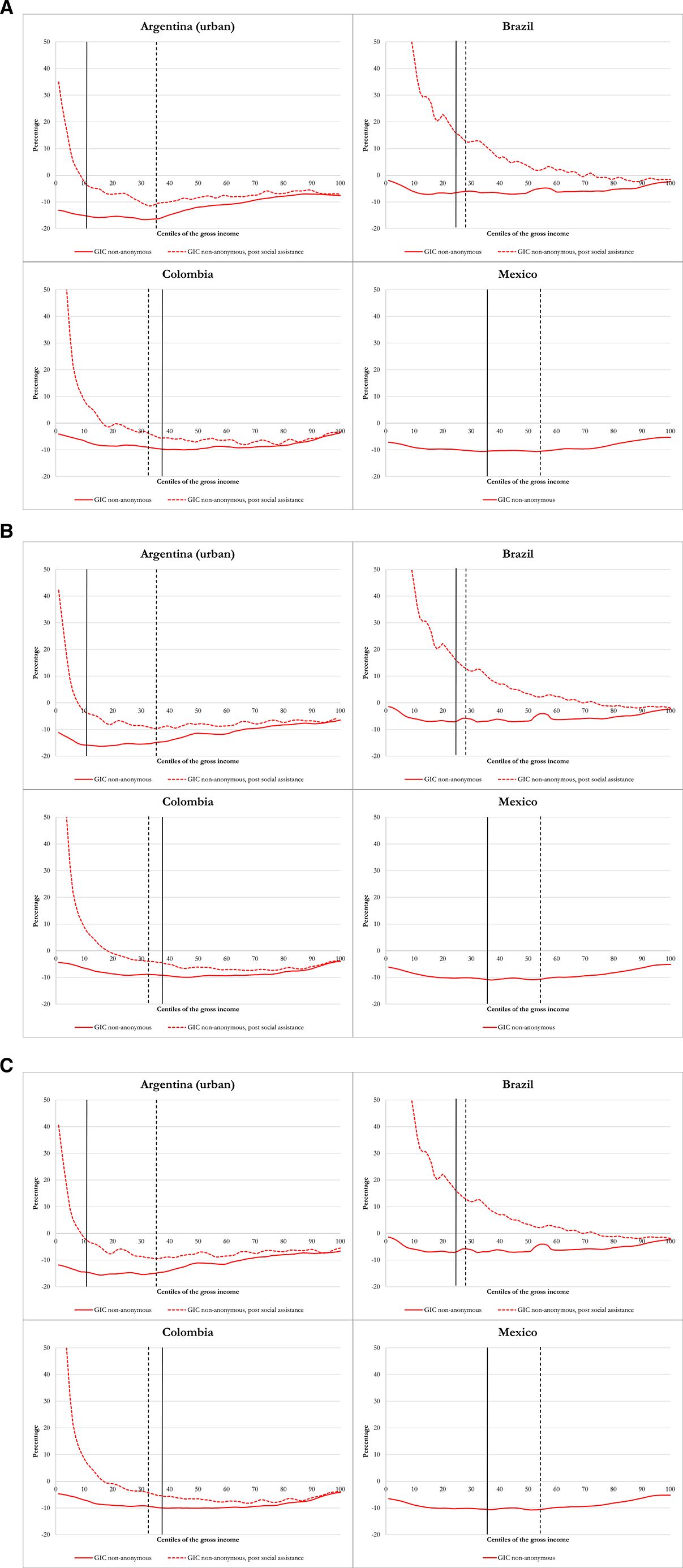

Non-anonymous Growth Incidence Curves Panel (a) “Concentrated Losses” Scenario, Panel (B) “Dispersed Losses” Scenario, Panel (c) “Actual Losses” Scenario. Notes: The dashed vertical line is the national poverty line and the bold vertical line is the $5.50 (moderate poor) per day international line (in 2011 PPP). Poverty lines based on the pre-pandemic distribution of income. Source: Authors’ calculations based on ENIGH (2018), EPH (2019), GEIH (2019), PNADC (2019).
The bold lines in Figure 2 show that households across the entire income distribution are worse off on average (regardless of the scenario) after the pandemic, which is not surprising, but the losses tend to be higher for the middle deciles rather than the poorest, which perhaps is surprising. The latter reflects the fact that poorer households have a cushion given by the existing social assistance programs (the bottom area in Figure 1); it also reflects the fact that three types of income are both not at risk and concentrated at the top end of the pre-pandemic income distribution: social security pensions, salaries earned in the public sector, and labor earnings of white collar workers who are CEO’s, managers and researchers with internet access at home.31
The dotted lines in Figure 2 show the GIC curves after considering the effect of the expanded social assistance. As expected, social assistance cuts the losses and, indeed, increases the income of poor households by significantly more in Brazil where the mitigation policies have been much more ambitious compared to Argentina and Colombia. In all three countries that have new or expanded social assistance transfers those transfers favor the pre-pandemic poor.
3.3.2. Pre- to Post-Pandemic Income Mobility
Table 7 shows the results of the downward mobility across broad income classes. These income classes are: poor -- less than $3.20 per day; moderate poor -- between $3.20 and $5.50 per day; lower-middle class -- between $5.50 and $11.50 per day; middle class -- between $11.50 and $57.60 per day; and rich -- more than $57.60 per day.32 Specifically, Table 7 shows the downward mobility of the lower middle class and middle class caused by the crisis.33
Income Mobility
| Post-Pandemic Without Expanded Social Assistance | Post-Pandemic With Expanded Social Assistance | |||||
|---|---|---|---|---|---|---|
| Country | % of moderate poor who fall to poor | % of the vulnerable who fall to moderate poor or below | % of the middle class who fall to moderate poor or below | % of moderate poor who fall to poor | % of the vulnerable who fall to moderate poor or below | % of the middle class who fall to moderate poor or below |
| Panel (a) "Concentrated Losses" Scenario | ||||||
| Argentina (urban) | 22.6 | 20.8 | 6.2 | 19.2 | 19.0 | 5.8 |
| Brazil | 10.2 | 8.9 | 2.7 | 6.8 | 6.9 | 1.9 |
| Colombia | 9.7 | 11.5 | 4.9 | 9.3 | 11.1 | 4.8 |
| Mexico | 15.2 | 15.1 | 3.7 | 15.2 | 15.1 | 3.7 |
| Panel (b) "Dispersed Losses" Scenario | ||||||
| Argentina (urban) | 27.5 | 21.9 | 0.0 | 7.8 | 13.0 | 0.0 |
| Brazil | 10.2 | 8.3 | 0.0 | 1.3 | 2.3 | 0.0 |
| Colombia | 15.8 | 14.2 | 0.0 | 10.2 | 10.7 | 0.0 |
| Mexico | 18.1 | 16.9 | 0.0 | 18.1 | 16.9 | 0.0 |
| Panel (c) "Actual Losses" Scenario | ||||||
| Argentina (urban) | 27.4 | 24.5 | 0.0 | 10.6 | 15.3 | 0.0 |
| Brazil | 10.2 | 8.3 | 0.0 | 1.3 | 2.3 | 0.0 |
| Colombia | 17.1 | 15.3 | 0.0 | 12.5 | 12.8 | 0.0 |
| Mexico | 21.0 | 17.3 | 0.0 | 21.0 | 17.3 | 0.0 |
-
Note: Income groups in terms of 2011 PPP are: poor: below $3.20; moderate poor: between $3.20 and below $5.50 per day; vulnerable: between $5.50 and below $11.50 per day; and middle class: between $11.50 and below $57.60 per day.
-
Source: Authors’ calculations based on ENIGH (2018), EPH (2019), GEIH (2019), PNADC (2019).
The results show, for all scenarios, that large shares of the pre-pandemic poor fall into extreme poverty and large shares of the pre-pandemic lower-middle class fall into poverty. In the “concentrated losses” scenario, even some previously middle-class households fall into poverty, though this does not occur in the “dispersed losses” scenario (and the “actual losses” scenario) as the losses to any individual household are smaller and thus not sufficient to drive a previously middle-class household into poverty. The difference across scenarios in the impact of the newly introduced social assistance is much more striking in Argentina and Brazil. In the “concentrated losses” scenario, the new transfers offer only very small reductions in those who fall into extreme poverty or poverty. In this scenario, households are losing substantial amounts of income which the new social assistance is too small to replace. In the “dispersed losses” scenario, though, each losing household loses less income and the newly introduced social assistance seems to be sufficient to offset those losses and thus prevent households from falling into poverty.
4. Concluding Remarks
When the pandemic struck, the first set of exercises quantifying the impact on living standards was produced fast and assumed that income losses were proportional across the income distribution. But it quickly became evident that this assumption was invalid as households with members working in informal sectors or members without the ability to telework were affected more drastically, and some households were minimally affected or not at all. Thus, the challenge was to use scant data to quantify the pandemic impact on living standards fast but not assuming that income losses would be proportional. Here, we propose a methodology with relatively low information requirements and a parsimonious modeling framework, which is also sufficiently flexible to allow the refinement of the projected effects of the shock as more information becomes available. Our proposed methodology to estimate the impact of COVID-19 or other unprecedented macroeconomic shocks on living standards allows researchers to relax the equal loss assumption and incorporate distributional changes in the analysis.
Footnotes
1.
For a description of lockdowns by country see, for example, Pages et al. (2020) and Hale et al. (2021).
2.
See, for example, Lackner et al. (2021), Sumner et al. (2020), and Valensisi (2020).
3.
See, for example, Bottan et al. (2020), INEGI (2020), Universidad Iberoamericana (2021), World Bank (2020).
4.
Although in Acevedo et al. (2020), Delaporte et al. (2021), ECLAC (2021), Solidarity Research Network (2020) (for Brazil), Universidad de los Andes (2020) (for Colombia) and Vos et al. (2020) incomes do not contract proportionally, these studies do not provide non-anonymous analysis of income.
5.
For example, Issahaku and Abu (2020), Nafula et al. (2020), Seck (2020), Yimer et al. (2020), and Younger et al. (2020) apply our proposed methodology to estimate the distributional consequences of COVID-19 in Ghana, Kenya, Senegal, Ethiopia, and Uganda, respectively. Their results suggest that the pandemic has severe consequences on inequality and poverty in these countries, reverting any progress made during the previous years.
6.
Another option is to consult with government experts.
7.
Some studies use the ability of teleworking as a way to identify the employment/income that may not be at risk. See: Bartik et al. (2020); Delaporte and Peña, 2020, Dingel and Neiman (2020), Hatayama et al. (2020), and Saltiel (2020).
8.
The first reported estimates of aggregated GDP contractions were published in the IMF’s World Economic Outlook of April 2020.
9.
This is analogous to the non-anonymous growth incidence curves in Bourguignon (2011), albeit here describing a contraction. In Bourguignon (2011), the author also discusses the theoretical and practical differences between the standard anonymous comparisons and non-anonymous methods, including the ones we use here.
10.
This may result in some discrepancies with poverty estimates published in national and international databases such as the World Bank’s PovcalNet.
11.
For Mexico and Colombia, we have information on these two incomes sources so we can test the sensitivity of results. Including consumption of own-production has little effect on the results as this is a small amount even for the poorest. What effect there is, however, is concentrated among poorest. The rental value of owner-occupied housing reduces the share of at-risk income roughly equally across the income distribution for both countries. Qualitatively, the results do not change when these two income sources are incorporated.
12.
The reforms are briefly described in Lustig and Scott (2019).
13.
Decree 297/2020 (Argentina), Decree 457 of March 22nd of 2020 (Colombia), and ILO Monitor: COVID-19 and the world of work (Brazil and Mexico). Table A1 in the appendix shows the distribution of employment between at-risk and not-at-risk by sector.
14.
Existing information suggests that international remittances in Latin America have not been negatively affected by the pandemic. In our four countries, remittances are important primarily for Mexico. Based on information from Banco de Mexico (2021), despite the crisis, income from remittances grew in 2020 compared to 2019.
15.
In the case of Argentina, the household survey does not allow us to identify internet access at home for white-collar workers. Thus, all of these workers were considered as not having their income at risk.
16.
We checked the robustness of our classification method by comparing the proportion of workers that can telework using our approach with that obtained by Delaporte and Peña (2020) for Latin American countries. Our results regarding the share of workers who can work from home are similar to that obtained by the latter (when they apply the approach from Saltiel (2020), the preferred one for developing countries). Furthermore, as far as we can tell, even the more appropriate approach has its limitations because not all workers who cannot telework should be assumed as having their income at risk, which seems to be the assumption in Delaporte and Peña (2020). Workers in essential sectors (healthcare, for example) will not have their incomes at risk even if they cannot telework. Thus, the approach we used here to classify incomes between at risk and not at risk appears to be more realistic because it includes the latter among the workers whose incomes are not at risk. In fact, Delaporte et al. (2021) do exactly that in a subsequent article. In addition, in our definition of incomes that are not at risk we also include nonlabor income such as income received from governments (as transfers or wages), remittances, and—except for rents--incomes from capital (e.g., interests and dividends) while Delaporte, Escobar, and Peña (2020) contemplate labor income only.
17.
Here we should note that the Argentina survey is urban only which may explain the somewhat difference shape compared to the other countries.
18.
Taking an average of the composition of gross income by decile we find that income at risk represents 26.5 percent, 20 percent, 34 percent, and 33 percent of total gross income in Argentina, Brazil, Colombia and Mexico, respectively.
19.
To estimate results, we rounded this up to 70 percent. Using a different indicator, Bottan et al. (2020) show that almost 80 percent of households reported loss of livelihood.
20.
To estimate results, we rounded it up to 60 percent. Bottan et al. (2020) show that approximately 70 percent of households reported loss of livelihood.
21.
The World Bank (2020) shows that in 2020 the share of households that experienced a decline in total income is 67.6 percent, on average, for Bolivia, Chile, Colombia, Costa Rica, Dominican Republic, Ecuador, Guatemala, Honduras, Paraguay, and Peru. Bottan et al. (2020) find that, on average, for a sample of seventeen countries from Latin America and the Caribbean, over 70 percent of respondents to an online/telephone survey conducted during 2020 reported decreases in income.
22.
We do not include employment support programs. Their impact is implicit in the projected aggregate contraction in the sense that the income of the beneficiary households of these programs is not at risk. In order to estimate the benefit of this policy, proper pre-policy counterfactuals need to be generated, which is beyond the scope of this paper. Thus, the contribution of government policies to mitigate the impact of the pandemic presented here may be a closer to a lower bound. For a more comprehensive description of programs that were introduced by the governments in the four countries examined here, see Blofield et al. (2021).
23.
Mexico neither expanded nor introduced new safety nets. There were really only two mitigation policies and neither involves an additional transfer: beneficiaries of the non-contributory pensions and scholarships were given two months in advance (with total payments for the year unchanged, at least for now) and access to ―credito a la palabra‖ (a loan without any guarantees) to mainly small and medium enterprises (which could become a transfer in retrospect if they are not paid back).
24.
For a more detailed description of the existing and new programs included in the simulations, see Table A2 in the Appendix.
25.
Estimates of inequality for outcomes yielding a similar aggregate decline in per capita gross income but all possible combinations of the two key parameters are available in Table A3 in the Appendix.
26.
The national poverty line in 2011 PPP a day is equivalent to $12.3 in Argentina, $6.3 in Brazil, $4.9 in Colombia, and $7.8 in Mexico. For Argentina, the conversion to 2011 PPP uses Buenos Aires city’s CPI because the one produced by the National Statistics Institute (INDEC) went through a series of methodological changes that weakened its credibility. See, for example, Cavallo (2013).
27.
Results for the squared poverty gap are shown in tables A5 and A6 in the Appendix.
28.
Estimates of poverty for outcomes yielding a similar aggregate decline in per capita gross income but all possible combinations of the two key parameters are available in Table A4 in the Appendix.
29.
As a check on the importance of the assumptions we have made about which income is at-risk, we repeated our analysis assuming that all income (except for income from cash transfers, pensions and government salaries) is at-risk. We find the results to be broadly similar, though the increases in poverty and inequality are slightly less when we restrict our attention to outcomes with income losses similar in scale to the IMF’s predictions for declines in GDP.
30.
As a check on the importance of including the change in the distribution of income on our poverty estimates, we repeated our analysis assuming that everybody’s income declines by the same per capita fall projected by the IMF for each country. In this case, the increase in the number of poor in the four countries taken together would equal 9.3 million (using the $5.50 poverty line).
31.
Figure A1 in the appendix shows both the anonymous and non-anonymous GICs. The anonymous GIC’s tend to be upward sloping (except for the very poorest) and lie below the non-anonymous ones. In fact, the decline of incomes at the bottom before the expanded social assistance is much larger especially for the ―concentrated losses‖ scenario because some of the households that were not among the poorest pre-pandemic end up with almost zero income.
32.
All cut-off values are in 2011 purchasing power parity (PPP) dollars. The default cut-off values $3.20 and $5.50 correspond to the income-category-specific poverty lines suggested in Jolliffe and Prydz (2016). The US$3.20 and US$5.50 PPP per day poverty lines are commonly used as extreme and moderate poverty lines for Latin America and roughly correspond to the median official extreme and moderate poverty lines in those countries. The $11.50 and $57.60 cutoffs correspond to cutoffs for the vulnerable and middle-class populations suggested for the 2005-era PPP conversion factors by López-Calva and Ortiz-Juarez (2014); $11.50 and $57.60 represent a United States CPI-inflation adjustment of the 2005-era $10 and $50 cutoffs. The US$10 PPP per day line is the upper bound of those vulnerable to falling into poverty (and thus the lower bound of the middle class) in three Latin American countries, calculated by López-Calva and Ortiz-Juarez (2014). Ferreira et al. (2013) find that an income of around US$10 PPP also represents the income at which individuals in various Latin American countries tend to self-identify as belonging to the middle class and consider this a further justification for using it as the lower bound of the middle class. The US$10 PPP per day line was also used as the lower bound of the middle class in Latin America in Birdsall (2010) and in developing countries in all regions of the world in Kharas (2010). The US$50 PPP per day line is the upper bound of the middle class proposed by Ferreira et al. (2013).
33.
The full set of income transition matrices is available upon request.
Appendix
Employment by Sector
| Panel (a) Argentina (urban) | |||
| Sector | Not at risk | At risk | Total |
| Agriculture | 65,109 | 0 | 65,109 |
| Mining | 36,897 | 12,281 | 49,178 |
| Manufacturing | 7,36,190 | 6,63,709 | 13,99,899 |
| Electricity, gas and water supply | 52,041 | 37,702 | 89,743 |
| Construction | 1,19,479 | 9,84,050 | 11,03,529 |
| Retail and wholesale | 5,93,180 | 15,84,484 | 21,77,664 |
| Accommodation and food service | 1,12,358 | 3,44,128 | 4,56,486 |
| Transport | 1,50,331 | 4,90,213 | 6,40,544 |
| Information and communication | 86,118 | 1,70,555 | 2,56,673 |
| Financial services | 1,78,675 | 88,681 | 2,67,356 |
| Real estate | 36,809 | 30,604 | 67,413 |
| Professional activities | 6,95,307 | 2,51,581 | 9,46,888 |
| Public administration | 10,16,020 | 0 | 10,16,020 |
| Education | 10,12,903 | 0 | 10,12,903 |
| Health | 7,93,233 | 0 | 7,93,233 |
| Other sectors | 3,49,785 | 14,04,260 | 17,54,045 |
| Total | 60,34,435 | 60,62,248 | 1,20,96,683 |
| % | 49.9% | 50.1% | |
| Panel (b) Brazil | |||
| Sector | Not at risk | At risk | Total |
| Agriculture | 86,36,764 | 0 | 86,36,764 |
| Mining | 3,84,819 | 28,358 | 4,13,177 |
| Manufacturing | 39,96,924 | 69,10,053 | 1,09,06,977 |
| Electricity, gas and water supply | 7,44,746 | 1,53,773 | 8,98,519 |
| Construction | 3,21,999 | 64,93,117 | 68,15,116 |
| Retail and wholesale | 83,52,357 | 95,43,628 | 1,78,95,985 |
| Accommodation and food service | 3,85,260 | 52,36,263 | 56,21,523 |
| Transport | 26,41,323 | 21,94,322 | 48,35,645 |
| Information and communication | 12,41,353 | 1,02,909 | 13,44,262 |
| Financial services | 11,03,351 | 1,68,406 | 12,71,757 |
| Real estate | 70,257 | 4,76,066 | 5,46,323 |
| Professional activities | 40,62,780 | 34,81,562 | 75,44,342 |
| Public administration | 51,11,266 | 0 | 51,11,266 |
| Education | 65,88,520 | 0 | 65,88,520 |
| Health | 47,47,906 | 0 | 47,47,906 |
| Other sectors | 6,98,142 | 1,06,02,821 | 1,13,00,963 |
| Total | 4,90,87,767 | 4,53,91,278 | 9,44,79,045 |
| % | 52.0% | 48.0% | |
| Panel (c) Colombia | |||
| Sector | Not at risk | At risk | Total |
| Agriculture | 35,15,167 | 0 | 35,15,167 |
| Mining | 1,95,612 | 1,222 | 1,96,834 |
| Manufacturing | 14,50,032 | 10,89,303 | 25,39,335 |
| Electricity, gas and water supply | 1,13,037 | 38,081 | 1,51,118 |
| Construction | 1,20,927 | 13,92,706 | 15,13,633 |
| Retail and wholesale | 16,32,476 | 28,15,331 | 44,47,807 |
| Accommodation and food service | 26,771 | 14,92,637 | 15,19,408 |
| Transport | 5,18,790 | 9,46,252 | 14,65,042 |
| Information and communication | 2,13,505 | 46,873 | 2,60,378 |
| Financial services | 3,05,304 | 26,567 | 3,31,871 |
| Real estate | 40,836 | 3,11,224 | 3,52,060 |
| Professional activities | 7,92,673 | 5,54,786 | 13,47,459 |
| Public administration | 7,11,302 | 0 | 7,11,302 |
| Education | 9,59,010 | 0 | 9,59,010 |
| Health | 9,56,935 | 0 | 9,56,935 |
| Other sectors | 2,05,906 | 16,88,689 | 18,94,595 |
| Total | 1,17,58,283 | 1,04,03,671 | 2,21,61,954 |
| % | 53.1% | 46.9% | |
| Panel (d) Mexico | |||
| Sector | Not at risk | At risk | Total |
| Agriculture | 89,53,313 | 0 | 89,53,313 |
| Mining | 1,98,514 | 0 | 1,98,514 |
| Manufacturing | 40,98,366 | 54,70,030 | 95,68,396 |
| Electricity, gas and water supply | 2,20,675 | 655 | 2,21,330 |
| Construction | 3,48,183 | 44,77,639 | 48,25,822 |
| Retail and wholesale | 58,93,101 | 51,45,482 | 1,10,38,583 |
| Accommodation and food service | 1,81,228 | 47,54,290 | 49,35,518 |
| Transport | 8,13,780 | 16,28,415 | 24,42,195 |
| Information and communication | 4,70,479 | 0 | 4,70,479 |
| Financial services | 5,58,741 | 557 | 5,59,298 |
| Real estate | 3,77,231 | 108 | 3,77,339 |
| Professional activities | 13,51,674 | 31,126 | 13,82,800 |
| Public administration | 21,72,350 | 0 | 21,72,350 |
| Education | 28,18,952 | 0 | 28,18,952 |
| Health | 16,70,654 | 0 | 16,70,654 |
| Other sectors | 62,08,673 | 55,66,657 | 1,17,75,330 |
| Total | 3,63,35,914 | 2,70,74,959 | 6,34,10,873 |
| % | 57.3% | 42.7% |
-
Source: Authors’ calculations based on ENIGH (2018), EPH (2019), GEIH (2019), PNADC (2019).
Description of Existing and New Social Assistance Programs by Country
| Argentina |
| NEW Ingreso Familiar de Emergencia is an unconditional transitory cash transfer to informal and vulnerable workers between 18 and 65 years old during the COVID-19 pandemic. The beneficiaries are individuals, and each household can receive only one allowance. Beneficiaries received three monthly payments of ARG $10,000 from May and July. The transfer amount represents 113.5% and 253.3% of the national and $5.5 PPP per day poverty lines. https://www.argentina.gob.ar/economia/medidas-economicas-COVID19/ingresofamiliardeemergencia |
| INCREASED Asignación Universal por Hijo is a conditional cash transfer program for children and adolescents (younger than 18 years old) living in poverty or vulnerability situations. The program includes conditions related to health and education obligations. The beneficiaries are individuals, and a household can receive up to 5 allowances. During the COVID-19 pandemic, the government announced a one-time extraordinary payment of ARG $3,100 in March. The transfer amount represents 35.2% and 78.5% of the national and $5.5 PPP per day poverty lines. https://www.anses.gob.ar/asignacion-universal-por-hijo https://www.argentina.gob.ar/economia/medidas-economicas-COVID19/bonos/AUH-AUE |
| Brazil |
| NEW Auxílio Emergencial is an unconditional transitory cash transfer to informal workers, individual microentrepreneurs, self-employed, and beneficiaries of Bolsa Família during the COVID-19 pandemic. The beneficiaries are individuals, and there are no restrictions on the number of allowances per household. Beneficiaries received five monthly payments of R $600 from April to August, and four monthly payments at half the original amount from September to December. The original transfer amount represents 121.9% and 140.3% of the national and $5.5 PPP per day poverty lines. https://www.caixa.gov.br/auxilio/PAGINAS/DEFAULT2.ASPX https://www.gov.br/cidadania/pt-br/servicos/sagi/relatorios/deolhonacidadania_3_2202.pdf |
| Colombia |
| NEW Ingreso Solidario is an unconditional transitory cash transfer program that aims to mitigate the situation of vulnerable households facing economic difficulties due to the COVID-19 pandemic. The beneficiaries of Ingreso Solidario are not obligated to any condition, but they must not be receiving any other social programs. The beneficiaries are households, and only one allowance per household is permitted. Beneficiarios received nine monthly payments of COL $160,000 from April to December. The program represents around 65.9% and 58.8% of the national and $5.5 PPP per day poverty lines. https://ingresosolidario.dnp.gov.co/ |
| NEW Bogotá Solidaria is an unconditional cash transfer program (from Bogotá’s Mayor Office) to support vulnerable and poor families in the city during the COVID-19 pandemic. The beneficiaries of Bogotá Solidario must not have any intra-household violence record. The beneficiaries are households, and only one allowance per household is permitted. Beneficiaries received five payments of COL $233,000. The program represents around 95.9% and 85.6% of the national and $5.5 PPP per day poverty lines. https://rentabasicabogota.gov.co/ |
| INCREASED Familias en Acción is a conditional cash transfer program for children and adolescents (younger than 18 years old) living under food insecurity conditions. The beneficiaries are individuals, and a household can receive up to 3 allowances. The program includes conditions related to health and education obligations. During the COVID-19 pandemic, the government announced five extraordinary payments of COL $145,000 delivered every two months between March and December. The program represents around 59.7% and 53.2% of the national and $5.5 PPP per day poverty lines. https://prosperidadsocial.gov.co/sgpp/transferencias/familias-en-accion/ https://prosperidadsocial.gov.co/asi-vamos-contra-el-covid-19/ |
| INCREASED Jóvenes en Acción is a conditional cash transfer program for young adults (between 16 to 24 years old) facing economic difficulties to continue or finish their studies. The program includes conditions related to eligibility criteria on other programs such as Familias en Accion and Red de la Superación de la Pobreza Extrema. The beneficiaries are individuals, and there are no restrictions on the number of allowances per household. During the COVID-19 pandemic, the government announced five-time extraordinary payments of COL $356,000 delivered every two months between March and December. The program represents around 146.5% and 130.7% of the national and $5.5 PPP per day poverty lines. https://prosperidadsocial.gov.co/sgpp/transferencias/jovenes-en-accion/ https://prosperidadsocial.gov.co/asi-vamos-contra-el-covid-19/ |
| INCREASED Colombia Mayor is an unconditional cash transfer program for older adults without a pension or who live in extreme poverty or indigence. The beneficiaries are individuals, and there are no restrictions on the number of allowances per household. During the COVID-19 pandemic, the government announced five-time extraordinary payments of COL $160,000 delivered every two months between March and December. The program represents around 65.9% and 58.8% of the national and $5.5 PPP per day poverty lines. https://prosperidadsocial.gov.co/Noticias/disponible-pago-ordinario-y-extraordinario-para-beneficiarios-de-colombia-mayor/ |
Gini Coefficient for Scenarios with Losses Similar to the Loss Projections by IMF (2021)
| Pre-Pandemic | Post-Pandemic Without Expanded Social Assistance | Post-Pandemic With Expanded Social Assistance | ||||
|---|---|---|---|---|---|---|
| Country | Scenario | Gini Coefficient | Gini Coefficient | Change (Gini points) | Gini Coefficient | Change (Gini points) |
| Argentina (urban) | 40% lose 90% | 44.4 | 48.6 | 4.2 | 46.9 | 2.5 |
| Argentina (urban) | 50% lose 70% | 44.4 | 47.7 | 3.3 | 46.0 | 1.6 |
| Argentina (urban) | 60% lose 60% | 44.4 | 47.5 | 3.0 | 45.7 | 1.3 |
| Argentina (urban) | 70% lose 50% | 44.4 | 47.0 | 2.6 | 45.3 | 0.9 |
| Argentina (urban) | 90% lose 40% | 44.4 | 46.7 | 2.2 | 45.1 | 0.7 |
| Brazil | 20% lose 80% | 55.4 | 57.0 | 1.6 | 53.3 | -2.1 |
| Brazil | 30% lose 50% | 55.4 | 56.4 | 1.1 | 52.7 | -2.6 |
| Brazil | 40% lose 40% | 55.4 | 56.4 | 1.0 | 52.7 | -2.7 |
| Brazil | 50% lose 30% | 55.4 | 56.2 | 0.8 | 52.5 | -2.8 |
| Brazil | 80% lose 20% | 55.4 | 56.1 | 0.8 | 52.5 | -2.9 |
| Colombia | 20% lose 100% | 55.0 | 58.2 | 3.1 | 56.9 | 1.9 |
| Colombia | 30% lose 70% | 55.0 | 57.2 | 2.2 | 56.0 | 1.0 |
| Colombia | 40% lose 50% | 55.0 | 56.6 | 1.6 | 55.5 | 0.4 |
| Colombia | 50% lose 40% | 55.0 | 56.4 | 1.4 | 55.2 | 0.2 |
| Colombia | 70% lose 30% | 55.0 | 56.2 | 1.2 | 55.1 | 0.1 |
| Colombia | 100% lose 20% | 55.0 | 56.0 | 0.9 | 54.8 | -0.2 |
| Mexico | 30% lose 80% | 46.4 | 49.3 | 2.9 | 49.3 | 2.9 |
| Mexico | 40% lose 60% | 46.4 | 48.6 | 2.2 | 48.6 | 2.2 |
| Mexico | 50% lose 50% | 46.4 | 48.3 | 1.9 | 48.3 | 1.9 |
| Mexico | 60% lose 40% | 46.4 | 47.9 | 1.5 | 47.9 | 1.5 |
| Mexico | 80% lose 30% | 46.4 | 47.7 | 1.3 | 47.7 | 1.3 |
-
Notes: Change is the difference between post- and pre-pandemic Gini coefficients.
-
Source: Authors’ calculations based on ENIGH (2018), EPH (2019), GEIH (2019), PNADC (2019).
Incidence of Poverty for with Losses Similar to the Loss Projections by IMF (2021)
| Pre-Pandemic | Post-Pandemic Without Expanded Social Assistance | Post-Pandemic With Expanded Social Assistance | ||||||
|---|---|---|---|---|---|---|---|---|
| Country | Scenario | Headcount ratio (%) | Headcount ratio (%) | Change (pp.) | New poor (in millions) | Headcount ratio (%) | Change (pp.) | New poor (in millions) |
| Panel (a) National Poverty Line | ||||||||
| Argentina (urban) | 40% lose 90% | 35.5 | 42.8 | 7.2 | 2 | 40.3 | 4.8 | 1.4 |
| Argentina (urban) | 50% lose 70% | 35.5 | 42.9 | 7.4 | 2.1 | 40.3 | 4.7 | 1.3 |
| Argentina (urban) | 60% lose 60% | 35.5 | 43.1 | 7.6 | 2.1 | 40.6 | 5.1 | 1.4 |
| Argentina (urban) | 70% lose 50% | 35.5 | 43 | 7.4 | 2.1 | 40.7 | 5.2 | 1.5 |
| Argentina (urban) | 90% lose 40% | 35.5 | 43.1 | 7.6 | 2.1 | 40.7 | 5.1 | 1.4 |
| Brazil | 20% lose 80% | 28.2 | 31.8 | 3.6 | 7.5 | 26.1 | -2 | -4.3 |
| Brazil | 30% lose 50% | 28.2 | 31 | 2.8 | 5.8 | 25.2 | -3 | -6.2 |
| Brazil | 40% lose 40% | 28.2 | 31.1 | 3 | 6.2 | 25.1 | -3 | -6.3 |
| Brazil | 50% lose 30% | 28.2 | 30.9 | 2.7 | 5.6 | 24.8 | -3.3 | -6.9 |
| Brazil | 80% lose 20% | 28.2 | 31 | 2.9 | 6 | 24.9 | -3.3 | -6.8 |
| Colombia | 20% lose 100% | 31.8 | 36.9 | 5.2 | 2.5 | 34.8 | 3 | 1.5 |
| Colombia | 30% lose 70% | 31.8 | 37.1 | 5.3 | 2.6 | 35 | 3.2 | 1.6 |
| Colombia | 40% lose 50% | 31.8 | 36.5 | 4.7 | 2.3 | 34.4 | 2.6 | 1.3 |
| Colombia | 50% lose 40% | 31.8 | 36.5 | 4.7 | 2.3 | 34.2 | 2.4 | 1.2 |
| Colombia | 70% lose 30% | 31.8 | 36.4 | 4.6 | 2.3 | 34.1 | 2.3 | 1.1 |
| Colombia | 100% lose 20% | 31.8 | 36 | 4.2 | 2.1 | 33.4 | 1.7 | 0.8 |
| Mexico | 30% lose 80% | 53.8 | 58.6 | 4.9 | 6.1 | 58.6 | 4.9 | 6.1 |
| Mexico | 40% lose 60% | 53.8 | 59 | 5.2 | 6.5 | 59 | 5.2 | 6.5 |
| Mexico | 50% lose 50% | 53.8 | 59.5 | 5.7 | 7.1 | 59.5 | 5.7 | 7.1 |
| Mexico | 60% lose 40% | 53.8 | 59.3 | 5.5 | 6.9 | 59.3 | 5.5 | 6.9 |
| Mexico | 80% lose 30% | 53.8 | 59.3 | 5.5 | 6.9 | 59.3 | 5.5 | 6.9 |
| Panel (b) $5.5 PPP Poverty Line | ||||||||
| Argentina (urban) | 40% lose 90% | 10.9 | 19.1 | 8.2 | 2.3 | 16.8 | 5.9 | 1.7 |
| Argentina (urban) | 50% lose 70% | 10.9 | 18 | 7.1 | 2 | 14.9 | 4 | 1.1 |
| Argentina (urban) | 60% lose 60% | 10.9 | 17.5 | 6.6 | 1.9 | 13.9 | 3 | 0.9 |
| Argentina (urban) | 70% lose 50% | 10.9 | 16.5 | 5.6 | 1.6 | 13 | 2.1 | 0.6 |
| Argentina (urban) | 90% lose 40% | 10.9 | 15.8 | 4.9 | 1.4 | 12.8 | 1.9 | 0.5 |
| Brazil | 20% lose 80% | 25.4 | 28.9 | 3.5 | 7.4 | 22.2 | -3.2 | -6.7 |
| Brazil | 30% lose 50% | 25.4 | 27.9 | 2.6 | 5.4 | 21 | -4.4 | -9.1 |
| Brazil | 40% lose 40% | 25.4 | 27.9 | 2.5 | 5.3 | 21 | -4.4 | -9.2 |
| Brazil | 50% lose 30% | 25.4 | 27.5 | 2.1 | 4.5 | 20.6 | -4.7 | -9.9 |
| Brazil | 80% lose 20% | 25.4 | 27.6 | 2.2 | 4.6 | 20.6 | -4.7 | -9.9 |
| Colombia | 20% lose 100% | 37.6 | 42.6 | 5 | 2.5 | 40.8 | 3.2 | 1.6 |
| Colombia | 30% lose 70% | 37.6 | 42.7 | 5.2 | 2.5 | 41.1 | 3.5 | 1.7 |
| Colombia | 40% lose 50% | 37.6 | 42.3 | 4.8 | 2.3 | 40.6 | 3 | 1.5 |
| Colombia | 50% lose 40% | 37.6 | 42.2 | 4.7 | 2.3 | 40.4 | 2.9 | 1.4 |
| Colombia | 70% lose 30% | 37.6 | 42.1 | 4.5 | 2.2 | 40.3 | 2.7 | 1.3 |
| Colombia | 100% lose 20% | 37.6 | 41.8 | 4.2 | 2.1 | 39.8 | 2.2 | 1.1 |
| Mexico | 30% lose 80% | 34.9 | 41.6 | 6.8 | 8.5 | 41.6 | 6.8 | 8.5 |
| Mexico | 40% lose 60% | 34.9 | 41.8 | 6.9 | 8.7 | 41.8 | 6.9 | 8.7 |
| Mexico | 50% lose 50% | 34.9 | 42.1 | 7.3 | 9.1 | 42.1 | 7.3 | 9.1 |
| Mexico | 60% lose 40% | 34.9 | 41.6 | 6.7 | 8.4 | 41.6 | 6.7 | 8.4 |
| Mexico | 80% lose 30% | 34.9 | 41.3 | 6.5 | 8.1 | 41.3 | 6.5 | 8.1 |
-
Notes: Change is the difference between post- and pre-pandemic headcount ratios. The number of new poor is calculated as the change in post- and pre-pandemic headcount ratios times the projected population for 2020 obtained from the World Bank World Development Indicators. pp: percentage points.
-
Source: Authors’ calculations based on ENIGH (2018), EPH (2019), GEIH (2019), PNADC (2019).
Squared Poverty Gap, National Poverty Line
| Pre-Pandemic | Post-Pandemic Without Expanded Social Assistance | Post-Pandemic With Expanded Social Assistance | |||
|---|---|---|---|---|---|
| Country | Squared poverty gap (%) | Squared poverty gap (%) | Change (pp.) | Squared poverty gap (%) | Change (pp.) |
| Panel (a) "Concentrated Losses" Scenario | |||||
| Argentina (urban) | 7.8 | 13.9 | 6.1 | 11.6 | 3.8 |
| Brazil | 9 | 10.9 | 2 | 5.9 | -3 |
| Colombia | 8.9 | 14 | 5 | 12.2 | 3.3 |
| Mexico | 10.7 | 15.2 | 4.5 | 15.2 | 4.5 |
| Panel (b) "Dispersed Losses" Scenario | |||||
| Argentina (urban) | 7.8 | 10.8 | 3 | 8.7 | 1 |
| Brazil | 9 | 9.7 | 0.7 | 5.1 | -3.8 |
| Colombia | 8.9 | 10 | 1.1 | 8.5 | -0.4 |
| Mexico | 10.7 | 13.3 | 2.6 | 13.3 | 2.6 |
| Panel (c) "Actual Losses" Scenario | |||||
| Argentina (urban) | 7.8 | 11.1 | 3.3 | 9 | 1.2 |
| Brazil | 9 | 9.7 | 0.7 | 5.1 | -3.8 |
| Colombia | 8.9 | 10.3 | 1.3 | 8.7 | -0.2 |
| Mexico | 10.7 | 13.6 | 2.9 | 13.6 | 2.9 |
-
Note: Change is the difference between post- and pre-pandemic squared poverty gaps. pp: percentage points.
-
Source: Authors’ calculations based on ENIGH (2018), EPH (2019), GEIH (2019), PNADC (2019).
Squared Poverty Gap, $5.5 PPP Poverty Line
| Pre-Pandemic | Post-Pandemic Without Expanded Social Assistance | Post-Pandemic With Expanded Social Assistance | |||
|---|---|---|---|---|---|
| Country | Squared poverty gap (%) | Squared poverty gap (%) | Change (pp.) | Squared poverty gap (%) | Change (pp.) |
| Panel (a) "Concentrated Losses" Scenario | |||||
| Argentina (urban) | 2.2 | 6.1 | 3.9 | 3.9 | 1.8 |
| Brazil | 7.7 | 9.5 | 1.8 | 4.7 | -3 |
| Colombia | 11.1 | 16.2 | 5.1 | 14.4 | 3.2 |
| Mexico | 6 | 9.7 | 3.7 | 9.7 | 3.7 |
| Panel (b) "Dispersed Losses" Scenario | |||||
| Argentina (urban) | 2.2 | 3 | 0.8 | 1.8 | -0.4 |
| Brazil | 7.7 | 8.3 | 0.6 | 4 | -3.7 |
| Colombia | 11.1 | 12.4 | 1.2 | 10.8 | -0.4 |
| Mexico | 6 | 7.6 | 1.6 | 7.6 | 1.6 |
| Panel (c) "Actual Losses" Scenario | |||||
| Argentina (urban) | 2.2 | 3.2 | 1 | 1.8 | -0.3 |
| Brazil | 7.7 | 8.3 | 0.6 | 4 | -3.7 |
| Colombia | 11.1 | 12.6 | 1.5 | 11 | -0.1 |
| Mexico | 6 | 7.9 | 1.9 | 7.9 | 1.9 |
-
Note: Change is the difference between post- and pre-pandemic squared poverty gaps. pp: percentage points.
-
Source: Authors’ calculations based on ENIGH (2018), EPH (2019), GEIH (2019), PNADC (2019).
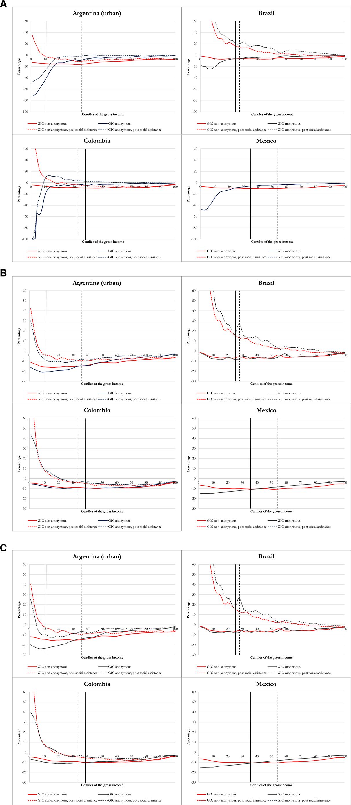

Anonymous and Non-anonymous Growth Incidence Curves Panel (a) “Concentrated Losses” Scenario, Panel (b) “Dispersed Losses” Scenario, Panel (c) “Actual Losses” Scenario Notes: The dashed vertical line is the national poverty line and the bold vertical line is the $5.50 (moderate poor) per day international line (in 2011 PPP). Poverty lines based on the pre-pandemic distribution of income. Source: Authors’ calculations based on ENIGH (2018), EPH (2019), GEIH (2019), PNADC (2019).
References
-
1
Implicaciones Sociales Del COVID-19: Estimaciones y Alternativas Para América Latina y El CaribeDocumento de discusión del BID, (820.
- 2
-
3
The impact of COVID-19 on small business outcomes and expectationsProceedings of the National Academy of Sciences of the United States of America 117:17656–17666.https://doi.org/10.1073/pnas.2006991117
-
4
Equity in a Globalizing WorldThe (indispensable) middle class in developing countries; or, the rich and the rest, not the poor and the rest, Equity in a Globalizing World, World Bank.
- 5
-
6
The Unequal Burden of the Pandemic: Why the Fallout of COVID-19 Hits the Poor the HardestInter-American Development Bank.
-
7
Status quo in the welfare analysis of tax reformsReview of Income and Wealth 57:603–621.https://doi.org/10.1111/j.1475-4991.2011.00480.x
-
8
Online and official price indexes: Measuring Argentina’s inflationJournal of Monetary Economics 60:152–165.https://doi.org/10.1016/j.jmoneco.2012.10.002
-
9
The Distributional Consequences of Social Distancing on Poverty and Labour Income Inequality in Latin America and the CaribbeanJ Popul Econ 34:1385–1443.https://doi.org/10.1007/s00148-021-00854-1
-
10
Working from Home Under COVID-19: Who Is Affected? Evidence from Latin American and Caribbean CountriesCEPR Covid Economics.
-
11
How many jobs can be done at home?Journal of Public Economics 189:104235.https://doi.org/10.1016/j.jpubeco.2020.104235
- 12
-
13
Instituto Nacional de Estadística y Geografía de MéxicoEncuesta Nacional de Ingresos y Gastos de Los Hogares, Instituto Nacional de Estadística y Geografía de México.
-
14
Instituto Nacional de Estadística y Censos de ArgentinaEncuesta Permanente de Hogares, Instituto Nacional de Estadística y Censos de Argentina.
- 15
-
16
Gran Encuesta Integrada de HogaresDepartamento Administrativo Nacional de Estadística de Colombia.
-
17
A global panel database of pandemic policies (Oxford COVID-19 Government Response Tracker)Nature Human Behaviour 5:529–538.https://doi.org/10.1038/s41562-021-01079-8
-
18
Jobs’ Amenability to Working from Home: Evidence from Skills Surveys for 53 CountriesJobs’ Amenability to Working from Home: Evidence from Skills Surveys for 53 Countries, Vol, 9241, 10.1596/1813-9450-9241.
-
19
ILO Monitor: COVID-19 and the World of WorkILO Monitor: COVID-19 and the World of Work, 2nd, ed, International Labor Organization, https://www.ilo.org/global/topics/coronavirus/impacts-and-responses/WCMS_740877/lang--en/index.htm.
- 20
- 21
-
22
COVID-19 in Ghana: Consequences for Poverty, and Fiscal ImplicationsAfrican Economic Research Consortium. Working Paper.
- 23
- 24
- 25
-
26
How Much Does Reducing Inequality Matter for Global Poverty?The World Bank.https://doi.org/10.1596/33902
-
27
A vulnerability approach to the definition of the middle classThe Journal of Economic Inequality 12:23–47.https://doi.org/10.1007/s10888-012-9240-5
-
28
Política fiscal para un Estado de bienestarNexos. Julio.
-
29
Poverty and Distributional Effects of COVID-19 on Households in KenyaAfrican Economic Research Consortium. Working Paper.
- 30
-
31
Pesquisa Nacional Por Amostra de Domicilios ContinuaInstituto Brasileiro de Geografia e Estatistica do Brasil.
-
32
Measuring Aggregate Welfare in Developing Countries: How Well Do National Accounts and Surveys Agree?Review of Economics and Statistics 85:645–652.https://doi.org/10.1162/003465303322369786
- 33
-
34
Poverty Consequences of COVID-19 Epidemic-Induced Lockdowns in Senegal: Extent and Implications from a Household SurveyAfrican Economic Research Consortium. Working Paper.
- 35
-
36
Precarity and the pandemic: COVID-19 and poverty incidence, intensity, and severity in developing countriesWIDER Working Paper 2020/77.
-
37
La Vulnerabilidad del Empleo a la Emergencia de COVID19 Nota Macroeconómica 11Macroeconomics research group, Universidad de los Andes.
-
38
Encuesta de Seguimiento de los Efectos del COVID-19 en el Bienestar de los Hogares MexicanosUniversidad Iberoamericana, México.
-
39
WIDER Working PaperCOVID-19 and global poverty: Are LDCs being left behind?, WIDER Working Paper, 10.35188/UNU-WIDER/2020/830-6.
- 40
-
41
COVID-19 High-Frequency Monitoring DashboardThe World Bank.
-
42
The Short-Run Impact of the COVID-19 Crisis on Poverty in EthipiaAfrican Economic Research Consortium. Working Paper.
- 43
Article and author information
Author details
Valentina Martinez Pabon

Funding
This paper was prepared as part of the Commitment to Equity Institute’s research program and benefitted from the generous support of the Bill & Melinda Gates Foundation.
Acknowledgements
An earlier version of this paper appeared in “Covid Economics: Vetted and Real-Time Papers,” Issue 46, Center for Economic Policy Research (CEPR). The authors are very grateful to François Bourguignon, Raymundo Campos, Mercedes D’Alessandro and colleagues in Argentina’s Ministry of Economy, Cristina Fernandez, Carlos Grushka, Daniel Heymann, Rafael Rofman, John Scott, Sergei Soares, and Mariano Tommasi, and anonymous peer-reviewers from CEPR’s COVID Economics and CGD’s Working Papers Series. The authors are also grateful to the participants of the 8th Congress of the International Microsimulations Association (virtual), December 1, 2021. All errors remain our sole responsibility.
Publication history
- Version of Record published: April 30, 2023 (version 1)
Copyright
© 2023, Lustig et al.
This article is distributed under the terms of the Creative Commons Attribution License, which permits unrestricted use and redistribution provided that the original author and source are credited.