Stay on Target: Population Projections and Microsimulation Design
- Center for Mind and Culture, United States
- University College London, United Kingdom
- NORCE Center for Modelling Social Systems, Norway
Abstract
Even though standard cohort component models are relatively easy to comprehend, designing simulations to match expected population estimates and projections in multiple countries and over long spans of time is surprisingly challenging. We identify microsimulation design options that replicate United Nations population estimates and projections in three countries (Norway, United States, and India) over a 150-year time span. The design adapts the United Nations cohort component model, which implies a certain ordering of demographic events, and uses either cohorts or age groups to assign risk. We design four simple microsimulations that use United Nations demographic statistics as exogenous variables. One model adjusts event ordering and assignment of risk by age, called the Split Fertility design, and one model does not. Each model operates in either one- or five-year steps. The Split Fertility design has less than one percent divergence in total births, deaths, and population in all three countries. The simpler design produces varying magnitudes of divergence, as large as 20% in India. The Split Fertility design is suitable for simulations that seek to maintain population dynamics in multiple countries, whether operating in one- or five-year steps. The Split Fertility design is ideal for comparative simulations that adapt demographic statistics from cohort component models. Development of the design highlights the flexibility of simulations and the importance of careful interpretation of exogenous statistics in simulation design.
1. Introduction
As computing capabilities expand, simulations can model complex processes among larger populations of artificial agents over longer periods of time (Anderson and Hicks, 2011). Agents can represent actual populations in a given region, where they are assigned characteristics (e.g., sex, ethnicity), engage in relevant behaviors (e.g., marriage, having children), and age as time advances. Research questions drive the specific design and outcome variables of a simulation, including the implementation of demographic processes. For some projects, modeling population change is central, while in others it is only a background process. In the latter case, a popular option is using demographic rates as exogenous variables, so that agents experience demographic events as state transitions (e.g. dying or giving birth) determined by an external statistic. This approach seems straightforward, but simulation design is highly flexible and there is a veritable host of implementation options for demographic events (for overviews of demographic microsimulations and their options, see: Birkin and Wu, 2012; Li and O’Donoghue, 2013; Mason, 2014; Morand et al., 2010; Spielauer, 2011; Van Imhoff and Post, 1998; Zagheni, 2015; Zaidi and Rake, 2001). Even when using high-quality exogenous variables, microsimulations can produce unexpectedly divergent outcomes (Li and O’Donoghue, 2014).
We identify a set of simulation design options, called Split Fertility, which replicate the United Nations (UN) 2019 World Population Prospects estimates and projections in multiple countries over the 1950-2100 period. Our design adapts the UN cohort component model (CCM), which operates under specific assumptions and with specific mortality, fertility, and migration statistics. Even though standard CCMs like the UN’s are relatively easy to comprehend, designing simulations to match UN estimates and projections in multiple countries and over long spans of time is surprisingly challenging. Guidance on how to adapt demographic statistics from a CCM to a microsimulation is sparse (a chapter on the topic in a SAS manual was only published in 2021) (Marois and KC, 2021), and the ‘black box’ of design decisions in existing complex demographic microsimulations is overwhelming (Dekkers, 2010). Knowledge of the mathematical relationships in demographic statistics is easily taken for granted, creating an invisible hurdle to overcome when designing a microsimulation from scratch.
When faced with a deluge of data sources and decision-making for microsimulation design, it is tempting to interpret statistics as the probability of experiencing an event for people in the displayed categories (e.g. women aged 20-24) (Van Imhoff and Post, 1998), and to use alignment procedures to correct divergence (Li and O’Donoghue, 2014). As we demonstrate, taking an intuitive interpretation of UN statistics in a microsimulation can produce very large population divergences in some countries, depending on prevailing population dynamics. Reducing that divergence requires a detailed understanding of how the UN’s demographic statistics produce expected population dynamics within a standard CCM. In particular, we implement the CCM’s implied ordering of demographic events, accommodate UN statistics that use cohorts instead of current age to assign risk, and make additional adjustments when converting between five- and one-year time steps.
The Split Fertility design closely matches UN CCM estimates and projections of population dynamics in multiple countries. Matching UN CCM population projections with a microsimulation approach is valuable for several reasons. It enables implementing population dynamics in all countries modeled by the UN, and it strengthens the validity of simulation model results against a well-regarded standard (Morrison, 2008). In this paper, we describe in detail why the design works, which makes it accessible to those unfamiliar with traditional demographic techniques and statistics. The Split Fertility design is sensible given a thorough understanding of UN statistics and assumptions, but not particularly intuitive. We therefore compare the Split Fertility design to a simpler microsimulation design and identify country-specific conditions that produce particularly high or low divergence from UN data. We make the Split Fertility design freely available to use as a demography module in a simulation of any country with UN population projection and estimation data.
Computational simulations of population change are extremely flexible in implementation. This means that they force into the open measurement assumptions latent within less flexible CCM projections, allowing demographers to take full responsibility for whatever assumptions they finally adopt. The possibility of competing implementation assumptions invites measures of the difference it makes to adopt one design option over alternatives. This paper quantifies this difference in a basic way, using the UN CCM as a standard for comparison. Importantly, multiple approaches are supported in computational simulation, another indication of the utility of simulation methods for demography.
2. Background
2.1 Population Dynamics and Dynamic Simulations
There is a variety of human population simulation models. Because our purpose is to replicate the UN CCM projections, we focus on dynamic microsimulation models (MSMs) that treat demographic statistics as exogenous variables. By dynamic, we are referring to MSMs that involve the passage of time and allow individual agents to age and for agent characteristics to change due to exogenous demographic rates (Li and O’Donoghue, 2013). Dynamic MSMs are similar to agent-based models (ABMs) in that both focus on the level of individual agents. However, agents in ABMs typically interact, respond to processes endogenous to the model, take account of individual differences in agents, and allow for relatively complex cognition and behavior. By contrast, the agents in MSMs are placeholders for the imposition of stipulated stochastic events, such as probabilities of transitions between states (e.g. dying, giving birth, migrating). Thus, the MSMs we consider represent a “top-down” approach to simulating population change, whereas ABMs typically emphasize “bottom-up” behaviors and interactions between individuals that produce non-linear feedback effects (Zagheni, 2015). It is possible to employ hybrid models that mix top-down and bottom-up components, and may include complex behaviors, interactions, and transition probabilities shaped by both micro- and macro-level variables (Bae et al., 2016; Birkin and Wu, 2012). For simplicity, we will refer to dynamic MSMs or hybrid models as simulations hereafter.
The implementation of demographic rates as exogenous variables that update as time advances is a popular option in many policy-focused simulations (Li and O’Donoghue, 2013). For instance, healthcare demand and social-care models simulate the need for, and availability of, family- or formal-sourced care for young or older populations over time (Gostoli and Silverman, 2020; Mielczarek and Zabawa, 2021; Spijker et al., 2022). When designing a simulation that treats population dynamics as exogenous, it is intuitive to use reliable demographic statistics that are easily accessible. Most simulations designed for a particular region or country use statistics from local governments. The DemoCare model, for example, is a hybrid model that follows cohorts of individuals as they age and are exposed to an exogenous risk of fertility and death, where the risk is determined by population statistics from Spain in 1908 to 1968 (Spijker et al., 2022).
Simulations that can use demographic statistics to model population outcomes in multiple countries are rare (for a notable exception, see Spielauer and Dupriez, 2019). One hindrance to comparative model design is the availability of standardized data and proper implementation of that data in different countries. The World Population Prospect reports from the UN provide fertility, mortality, migration, and total population statistics by age and sex for all countries across a 150-year timespan (United Nations, 2019). The UN datasets are therefore a unique source for multi-country and comparative simulations, and permit the use of exogenous statistics in simulations for both the past and future. The UN uses a CCM to connect past and future demographic statistics to the total expected population outcomes. However, there is little guidance on how to adapt the demographic information provided by the UN into a simulation. In the following sections, we review the UN’s methods and explain why simulations can diverge from the UN’s population outputs even when using intuitive designs and applying the UN’s demographic statistics as inputs.
2.2 The UN’s Demographic Statistics and the Cohort Component Method
The UN develops population estimates and projections for nearly every country, and they periodically revise their estimates and projections. As part of this effort, the UN painstakingly estimates past fertility, mortality, and migration for each country using demographic techniques that standardize statistics from government, survey, and other sources (United Nations, 2019). The UN’s 2019 revision uses Bayesian techniques and explicit assumptions about trends in fertility, mortality, and migration to calculate demographic statistics that cover future periods (2020-2100). The UN publishes variants of projections, or scenarios, based on different explicit assumptions. The Medium Variant projection scenario assumes birth rates will converge to a global medium, life spans will generally increase, and migration will continue at the count last observed for the 2015-2020 interval; these assumptions are consistent with contemporary demographic theory and are tractable at the global scale (United Nations, 2019). The UN therefore estimates demographic statistics for the 1950-2020 period retrospectively using observed data, and uses demographic theory and statistical techniques to derive future demographic statistics. The entire process is iterative and the UN must maintain a global net balance in population totals.
Despite variation in how the UN calculates each country’s estimates and projections from different data sources and methods, past and future demographic statistics operate seamlessly within the CCM to produce population totals for the entire 1950-2100 period. The UN’s CCM starts in 1950 with the estimate of total population by sex and five-year age groups, and moves forward in five-year intervals.1 The number of births is determined using age-specific fertility rates (ASFRs), a proportion of people in each age group survives based on survival ratios (SRs), and everyone is aged forward five years. The count of net migrants is also added or removed before the next five-year interval. Despite changes in how fertility, mortality, and migration statistics are derived in the estimation years (1950-2020) and the projection years (2020-2100), the CCM procedure can start from any five-year interval between 1950 and 2095 and be repeated until 2100 (United Nations, 2019).
The UN’s demographic data are high quality and freely available to use as exogenous variables in a simulation of any country’s population covering up to 150 years. The UN’s CCM procedure seems straightforward, suggesting that a match between simulation and CCM outcomes is simple to achieve. In fact, the rich implementation-assumption space of simulations surfaces complexities in the CCM procedure. The CCM has an implied ordering of demographic events and non-intuitive assignment of risk using cohorts. To understand these complexities, we must examine the demographic statistics used as inputs in the UN’s CCM model and the assumptions underlying time and age concepts.
2.3 Demographic Statistics, Event Ordering, and the Population at Risk
CCM and simulation approaches differ in how they assign the probability of experiencing an event at a given point in time (Van Imhoff and Post, 1998). In a simulation approach, agents have an individual probability of experiencing each event based on their characteristics (e.g. age, sex) and behaviors (if relevant; in the case of the MSMs in this paper, agent behaviors are not relevant). When operating with discrete time, the agent will experience an event instantaneously at a specific time. A major design decision is selecting the order that agents may experience events. Events can occur in a set order, in a random order for each agent, in an order where the higher probability event always occurs first, or with multi-step Monte Carlo experiments to determine the conditional probability of each event (for a discussion of competing risk in microsimulation, see Van Imhoff and Post, 1998). Event order can be decided based on theory, realism, the structure of the original data source, and/or for computational efficiency.
The structures of UN demographic statistics have consequences for selecting event ordering and assignment of risk by age for a simulation. Unlike individual-level probabilities in a simulation where events occur instantaneously in a given moment, many demographic statistics are in the form of an “occurrence/exposure” rate for a given period of time (Preston et al., 2000). That is, the number of occurrences (e.g. births) is the numerator, and the denominator is the number of people exposed to the risk (e.g. the female population of childbearing ages), over a time interval, such as five years. Membership of the population at risk can change within five years, because people simultaneously move in/out of the geographic area, die, age into a different risk group, or experience some other state change (Van Imhoff and Post, 1998). Demographic rates therefore use the mid-point population to identify the average population at risk and account for this alteration in the population at risk over time The mid-point population is the simple average of the population at time t and time t+5, where t is the starting year population (e.g. 1950) and t+5 is the population after all other events like mortality, aging, and migration have occurred (e.g., 1955) (Preston et al., 2000). Using the mid-point population can seem like ‘borrowing’ information from the future, which conflicts with a simulation approach in which time marches forward continually.
Consider the age-specific fertility rates (ASFRs), which represent the number of live births per year and per 1,000 females in an age group. The count of at-risk persons is the five year interval’s mid-point female population in the age group (e.g. average of those aged 20-24 in 1950 and in 1955). The ASFRs, therefore, represent the average risk of childbirth per year over a five-year interval, and presume information about the start and ending time point to identify the population at risk. Between time t and time t+5, some in the female population will die, migrate, and everyone will age each year, which moves them into a different age group’s fertility rate. In a simulation, the ASFRs will produce the wrong number of births if treated as a probability of birth occurring during the interval and if it is applied only once in a set order (e.g. always before or always after mortality), because there are either too many or too few agents in the population at risk at the given moment.
Some demographic statistics use birth cohort instead of age to describe the population at risk over a time interval. Using the cohort means group membership has a more permanent designation based on year of birth (e.g. those born in 1950-1954), rather than current age that advances each year. For instance, to identify how many people in a cohort survive from the beginning of a five-year interval to the next, the UN’s CCM uses the survival ratio (SR) statistic. The SR is calculated from an abridged life table, which is a classic tool used in demography to describe different pieces of information about how a birth cohort “dies out” over time (Preston et al., 2000). In a five-year CCM, the SR is the proportion of a cohort surviving from age x to x+5 from time t to t+5. The SR for males aged 20-24 in 1950, for example, describes the proportion that will survive into 1955 to become ages 25-29. Unlike the ASFRs that use a mid-point population, the SR applies to cohorts present at the beginning of the interval and to the newest cohorts born during the interval. The SR explicitly ignores changes in the population at risk when people enter or leave via migration. In a simulation, therefore, mortality should occur before aging and migration, and must occur after new births.
Migration statistics in CCM models can also rely on cohort designations, though some are designed as average exposure rates like ASFRs (Preston et al., 2000). In the case of the UN’s CCM, migration is best handled using cohorts, and the UN’s net migration statistic is provided as a count instead of a rate. The count of UN net migrants corresponds to the number of migrants to add or remove at the end of each five-year interval after everyone has been born, survived, and aged forward. This seems strange, but it is necessary because net migration is the residual between observed changes from natural increase (births minus deaths) and the total population at time t+5.2 The UN only published total net migrant counts by sex (not age) in the 2019 revision. Therefore, it is necessary to calculate the age distribution of net migrants by applying the CCM calculations before using the statistic in a simulation (see the appendix for our net-migration calculation procedure).3 Since migration is calculated after each cohort is aged forward, the cohort designations of net migrants match their age at the end of each five-year interval. In a simulation, migrants should be added or removed after mortality and aging.
Across all demographic events, differences in magnitude by age are apparent. Age groups may refer to the current age in any given year, or they may be birth cohort designations described by the population’s age at the beginning or end of the five-year interval. Users unfamiliar with conventional cohort designations may experience confusion when interpreting the age labels in UN data used to calculate CCMs. For instance, the UN lifetables show SR (column name is Sx,n) statistics for those of initial age 0, 1, and 5 on separate rows. It is not accurate to interpret these as applying to those aged 0-1, 1-4, and 5-9, respectively, and there are exceptions to interpreting them as the population’s initial age as well. The first entry for initial age “0” is the proportion of new cohorts born over the five-year interval (e.g. new births in 1950-54) who will survive to be the new 0-4 age group by the end (e.g. 1955). The SR for initial age “1” is the proportion of the population aged 0-4 at the start of the five-year interval who will survive to ages 5-9. The SR of initial age “5” does describe survivorship of those aged 5-9 at the beginning of the interval who will be 10-14 by the end. Subsequent initial ages in the life tables are interpreted similarly. This labeling may seem misleading but interpreting it this way ensures full coverage of both newborn and other young cohorts while distinguishing important differences in early life mortality risk. After calculating migration counts from a CCM procedure, it is also important to interpret the resulting age groups carefully. Migrants in the 0-4 group, for instance, refers to those who are age 0-4 at the end of the five-year period. Knowledge of how to interpret age groupings for each demographic event is important to assigning risk in a simulation to the appropriate set of agents and in the correct order.
With this more in-depth understanding of the implied event ordering of the UN’s demographic statistics in the CCM,4 designing a simulation that assigns risk to the appropriate population while operating prospectively is more complicated. How should a simulation use the UN’s statistics to maintain population dynamics at the individual level? As we will demonstrate, however, simply by adjusting the order of demographic events in a simulation, we can achieve an exact match with the UN’s expected births, deaths, and total population when operating in five-year time steps. Several more adjustments are necessary to achieve a close match when operating in one-year step, but we believe these adjustments are worth the effort, particularly in high-growth countries.
3. Two Demographic Microsimulation Designs
3.1 An Intuitive Interpretation
Not everyone who uses UN or similarly structured demographic statistics has a detailed understanding of the CCM method or how to interpret ASFRs, SRs, and net migration counts for a simulation. It is reasonable to assume that a simulation designer may attempt an intuitive approach first. For instance, consider an ‘Intuitive’ design that mimics how the UN’s CCM appears to order demographic events, and only uses current age to assign risk.5 This design is incorrect, but it serves as a useful foil for the correct approach. Suppose there is a version of the model that operates in five-year steps, and one that operates in one-year steps. The following demographic events occur in the specified order during each time step:
Fertility: female agents experience the full time step’s childbearing risk according to their current age and corresponding ASFR.
Mortality: agents experience death according to their current age and corresponding age labels for SR in the UN lifetable. Those who die are removed from the simulation.
Aging: surviving agents advance in age.
Migration: immigrants arrive and emigrants are removed from the simulation according to their current age and corresponding age labels for net migrants calculated from the UN data.
This design’s event ordering ignores the meaning of the mid-point population for the ASFRs, which uses exposure to account for the fact that all processes (births, deaths, migrations) are occurring simultaneously in real life. When applied to a simulation, the structure of the ASFR statistic suggests fertility occurs both before and after mortality, aging, and migration. When operating in a five-year step, this design will only be reliable when population dynamics maintain the size of female cohorts over time (e.g. a stationary one). If societal conditions favor a decline in females of high childbearing risk between the beginning and end of the five-year interval, there will be more births than expected. When the female population at elevated risk grows between the start and end of the interval, however, there will be fewer births than expected. When switching to a one-year step, the ASFR ordering problem is minimized because fertility occurs every year along with mortality, aging, and migration. Although the entire five-year fertility risk still favors female agents present before other demographic events occur, the magnitude of the problem is smaller.
The Intuitive design correctly places mortality before aging and migration after aging, which means that agents’ current age is the same as their cohort designations when mortality and migration occurs in the simulation. However, this is only true when operating in five-year steps. If current age is used to assign mortality and migration at the one-year step, then after the first one-year step, some agents will have a different cohort’s SR applied to them than intended by the CCM. Applying the SR according to current age will generally overestimate deaths because it exposes younger agents to higher rates of death prematurely. Applying the SR by current age will also underestimate infant deaths because newborn cohorts age out of their high-risk cohort designation too soon.6 The impact of incorrect assignment by age for migration is highly variable and depends on the age distribution of emigration and immigration for a given country and time. In general, migrants will leave or enter the simulation at a current age five years older than their cohort designation implies. That is, if an immigrant is arriving in 1950 to the “10” cohort designation, they should actually arrive as age “5” because their cohort corresponds to the age they will be in 1955, not 1950. Therefore, when cohort designation is interpreted as current age, migrants would be in an older age group when experiencing other demographic events.
Population dynamics are inherently connected, so higher or lower expected births leads to divergence in deaths and the size of the overall population, and the impact can compound with successive cohorts. If there are too few births over time, the cohorts of childbearing female agents will be smaller and there are even fewer births in later decades. Societal conditions can also reverse over time to favor too many births, deaths, or vice versa. Country-specific population dynamics, therefore, can produce very different profiles of divergence over a 150-year span.
3.2 The Split Fertility Design
So, what is the solution? We propose the Split Fertility design, which splits the fertility process so that childbearing happens twice instead of only once during each time step. At each round of the fertility process, that risk is halved according to the time steps of the model (e.g. 2.5 years of risk when operating in five-year steps, and 0.5 years of risk when operating in one-year steps). New agents born in the second round of fertility must immediately experience mortality and aging, so that they join their fellow infant cohort born in the first round of fertility. We summarize the order of events and assignment of risk in the Split Fertility design below:
The first round of fertility: female agents experience half of the childbearing risk for the time step according to their current age and corresponding ASFR.
Mortality: agents experience death according to their initial cohort age and corresponding age labels for SR in the UN data. Those who die are removed from the simulation.
Aging: surviving agents advance in age.
Migration: immigrants arrive and emigrants are removed from the simulation according to their ending cohort age and corresponding age labels for net migrants calculated from the UN data.
The second round of fertility: female agents experience another half of the childbearing risk for the time step according to their current age and corresponding ASFR.
Second round infant mortality and aging: only applies to new agents born in the second round of fertility.
By splitting the fertility risk, we replicate the mid-point population while also operating entirely prospectively. Doing so allows half of fertility risk to occur before mortality, aging, and migration, and half to occur after those events. Mortality and migration still occur in the order specified in the CCM, and to the appropriate age groups for a model operating in five-year steps.
When operating in one-year steps, however, we make additional adjustments to risk assignment by age to use cohort designations for mortality and migration events. As previously described, the SR applies to the cohort present at the beginning of each five-year interval and new births. The SR cohort designation generally matches current age at the beginning of each five-year interval. The cohort designations for migration counts, however, correspond to current age at the end of each five-year interval. This means that a one-year model must track agents’ current age, as well as starting and ending ages that match their cohort designations.7 Table 1 shows the age assignments for a hypothetical female agent aged 43 at the start of a five-year interval (t=0). Round two refers to the agent’s characteristics during the second round of fertility in the Split Fertility design, which occurs after mortality, migration, and the aging process. Starting age is set to match current age at t=0, and end age adds five years onto initial age. The values of starting and end age do not change until the next five-year interval. As shown, the fertility rate follows current age, the SR always matches the starting age, and the selection of migrants always corresponds to immigrant or emigrant agents’ end age.
Assignment of Demographic Event Risk by Age for 1-year Split Fertility Design
| t=0 | Rnd. 2 | t=1 | Rnd. 2 | t=2 | Rnd. 2 | t=3 | Rnd. 2 | t=4 | Rnd. 2 | |
|---|---|---|---|---|---|---|---|---|---|---|
| Agent Age Characteristics | ||||||||||
| Current Age | 43 | 44 | 44 | 45 | 45 | 46 | 46 | 47 | 47 | 48 |
| Starting Age | 43 | 43 | 43 | 43 | 43 | |||||
| Ending Age | 48 | 48 | 48 | 48 | 48 | |||||
| Corresponding Age Labels for UN Statistics | ||||||||||
| Fertility Rate | 40-44 | 40-44 | 40-44 | 45-49 | 45-49 | 45-49 | 45-49 | 45-49 | 45-49 | 45-49 |
| Survival Ratio | 40-44 | 40-44 | 40-44 | 40-44 | 40-44 | |||||
| Migration Count | 45-49 | 45-49 | 45-49 | 45-49 | 45-49 | |||||
Three other adjustments to the mortality and migration process are required to achieve the best fit to UN targets when operating in one-year steps. First, it is necessary to grant immigrants special immunity to death for the remaining years of each five-year interval. Since the SR only assigns risk to those present (or born) since the beginning of each five-year interval and immigrants arrive each year, they must be immune to death until the next interval starts.
The second and third adjustments apply to new cohorts born over a five-year interval to account for the uneven exposure to risk that newborn cohorts experience in their first five-year interval. It is helpful to visualize years of risk experienced by each newborn cohort as shown in Table 2, which resembles a simplified lexis diagram. Cohort “A” is born in the first year and is exposed to a full five-years of risk, while cohort “E” is born in the last year of a five-year interval and experiences only one-year of risk. When all years of risk (the cells in gray) are summed, there are 15 years of total risk across five newborn cohorts. In contrast, older cohorts would have all gray cells in the table filled in and experience 25 years of risk across five cohorts.
Years of Risk among Newborn Cohorts
| Cohort | Year 0 | Year 1 | Year 2 | Year 3 | Year 4 | Total Years of Risk | Percent of Total |
|---|---|---|---|---|---|---|---|
| A | 1 | 1 | 1 | 1 | 1 | 5 | 33 |
| B | 1 | 1 | 1 | 1 | 4 | 27 | |
| C | 1 | 1 | 1 | 3 | 20 | ||
| D | 1 | 1 | 2 | 13 | |||
| E | 1 | 1 | 7 | ||||
| Total | 15 | 100 |
It is intuitive to calculate yearly net migrants as the UN’s total count divided by 25 for older cohorts, resulting in an even distribution of migrants among all individual ages in each cohort. But among newborn cohorts, the yearly risk should be divided by 15. This adjustment effectively results in the first newborn cohort receiving about 1/3 of newborn cohorts’ total net migrants, and the last newborn cohort only about 7%.8 We must similarly adjust the calculation of mortality risk for newborn cohorts. Since the SR is expressed as probability of survival across a five-year interval, annual mortality risk among older cohorts is calculated by taking the UN SR to the fifth root and subtracting it from one. That is, the mortality rate (Model MR) for non-newborns is calculated as:
We estimate annual mortality risk among newborn cohorts by taking the third root of the SR instead, which accounts for the newborn cohorts experiencing only 15 out of the 25 total years of exposure over the five-year interval (i.e. 5 * 15/25 = 3). This is a simple adjustment that achieves a close fit to expected deaths while giving each newborn cohort differing exposure to risk over the five-year interval9 . Therefore, among newborn cohorts (SR[0]), the mortality rate is calculated as:
These adjustments are sensible with a thorough understanding of the UN’s statistics, but they are not intuitive. This is why the one-year version of the Intuitive design only uses current age to assign risk and doesn’t afford special treatment to infants’ calculation of risk or grant any immunities to immigrants. In the one-year Intuitive design, infant migrant counts and survival ratios are divided the same way as among agents in all other age groups. Contrasting the Intuitive and Split Fertility designs highlights the flexibility of simulations in implementing demographic statistics, and the importance of event ordering and how risk is assigned by age in a simulation.
4. Methods
4.1 Data
Data for MSM inputs and validation come from the UN’s 2019 World Population Prospects report for the countries of Norway, the United States (US), and India (United Nations, 2019). These three countries vary considerably in size and population dynamics over the 1950-2100 period. India is at an earlier stage of the demographic transition than the US and Norway. It has a much younger population and higher mortality risk in 1950 that drops quickly while fertility declines at a slower pace. Finally, India has much lower and net negative migration relative to its population size; although the US has relatively high net positive migration throughout the period, Norway achieves the highest net migrants relative to its population. These national differences challenge simulation-CCM matching in diverse ways. We downloaded UN data for each country on the population age/sex distribution, age-specific fertility rates, the abridged life table, infant sex ratios, as well as the total count of births, deaths, and net migrants.
4.2 Microsimulation Models
We designed four MSMs with AnyLogic 8.7.6: the Intuitive design in five-year steps and one-year steps, and the Split Fertility design in five-year steps and one-year steps. The Intuitive and Split Fertility designs differ in the ordering of demographic events and adjustments to the fertility rates, and the one-year versions differ in the risk assignment of agents by age. All models share common-sense adjustments to calculations when converting between annual and five-year periods of risk. The characteristics of each model and formulas are summarized in Table 3, and described in more detail below.
Model Design Characteristics and Formulas
| Intuitive Models | Split Fertility Models | |||
|---|---|---|---|---|
| Time | 5-year step and interval t =T= [1950,1955,…2100] | 1-year step t= [0,1,2,3,4], 5-year interval T=[1950,1955,…2100] | 5-year step and interval t =T= [1950,1955,…2100] | 1-year step t= (0,1,2,3,4), 5-year interval T=[1950,1955,…2100] |
| Event ordering | 0) Initialization, 1) fertility, 2) infant initialization, 3) mortality, 4) aging, 5) migration, 6) time step/interval advancement, T+5. | 0) Initialization, 1) fertility, 2) infant initialization, 3) mortality, 4) aging, 5) migration, 6) time step advancement, 7) repeat events 1-6 for t<5 until interval advancement, T+5. | 0) Initialization, 1) fertility (round one), 2) infant initialization (round one), 3) mortality, 4) aging, 5) migration 6) fertility round two, 7) infant initialization (round two), 8) second round infant mortality, 9) second round infant aging 10) time step/interval advancement, T+5. | 0) Initialization, 1) fertility (round one), 2) infant initialization (round one), 3) mortality, 4) aging, 5) migration 6) fertility round two, 7) infant initialization (round two), 8) second round infant mortality, 9) second round infant aging 10) time step advancement, 11) repeat events 1-10 for t<5 until interval advancement, T+5. |
| Current age (A) | 5-year age groups, A=[0,5…105] | 1-year age groups A=[0,1,…105] | 5-year age groups, A=[0,5…105] | 1-year age groups A=[0,1,…105] For immigrants: A=eA-t |
| Initial age (iA) | Not Applicable | Not Applicable | Not Applicable | iA=A-t |
| End age (eA) | Not Applicable | Not Applicable | Not Applicable | eA=A+(5-t) |
| Model Age-Specific Fertility Rates (ASFR) | ; Apply to current age (A) | ; Apply to current age (A) | ||
| Infant initialization | Assigned age -5, and sex based on UN sex ratio | Assigned age -1, and sex based on UN sex ratio | Assigned age -5, and sex based on UN sex ratio | Assigned age -1, and sex based on UN sex ratio. |
| Model Mortality Rate (MR) | 1 - (UNSR) | ; Apply to current age (A) | 1 - (UNSR) | ; Apply to initial age (iA). For newborn cohorts: ; For agents age 110+: 1. For immigrants: no mortality |
| Model Emigration count (EC) | (UNEC) * (Sample%) | ; Apply to current age (A) | (UNEC) * (Sample%) | ; Apply to end age (eA). For newborn cohorts: |
| Model Immigration count (IC) | (UNIC) * (Sample%) | ; Apply to current age (A) | (UNIC) * (Sample%) | ; Apply to end age (eA). For newborn cohorts: Note: All immigrants receive a tag to provide immunity to mortality and emigration. |
| Immigrant initialization | Assign current age (A) | Assign current age (A) | Assign current age (A) | Assign end age (eA), then calculate A and iA by subtracting remaining time steps and 5, respectively. |
| Period advance | NA | t + 1 | NA | t + 1 |
| Interval advance | T + 5, remove any tags that identify newborn cohorts or immigrant agents | |||
All four models are “top down” designs that use the sorting method for variance reduction (Bekkering, 1995; Van Imhoff and Post, 1998). To determine how many agents die and are born each time step, we apply the UN’s statistics as a rate to the size of the appropriate age/sex group of agents present at a given time. The resulting number of agents within the corresponding age/sex grouping are selected at random to experience the event. In the case of fertility, newborn agents are randomly assigned to female agents in the corresponding age group. For migration, we simply select the number to emigrate at random among the appropriate age/sex group, and initialize the number of immigrants as appropriate. The statistics update with every five-year interval, according to the availability of the UN data. The UN’s statistics are therefore exogenous, but the population at risk by age/sex characteristics is endogenous. This approach allows us to highlight the consequences of altering the event order and age assignment of risk, without interpreting random variation in the number of events as divergence from UN targets. Supplementary material in the appendix shows results using a more stochastic design (demographic rates and distributions are implemented as the probability of each agent experiencing the demographic event).
The statistics from the UN determine the age and sex distribution of the population at initialization and birth. Each simulation uses an initial sample of 100,000 agents, which is more efficient than running at full scale in each country, but still large enough to avoid substantial rounding errors common to the sorting method (Bekkering, 1995). At initialization, the sample of 100,000 agents matches the age and sex distributions of each country in 1950 according to UN data. In the five-year versions of the models, we use the UN’s data on sex and five-year age groups to initialize agent characteristics (i.e. agents are age 0, 5, 10, 15, etc.). In the one-year versions of the models, we use the UN’s data on sex and age in individual years to initialize agent characteristics (e.g. agents are age 0, 1, 2, 3, etc.).10 When new agents are born, they are assigned a sex to match the UN’s infant sex ratio.
For the fertility process, each model makes slight adjustments to the UN ASFRs, which originally express annual births per 1000 females over a five-year interval. In the one-year version of the Intuitive design, we simply divide the ASFRs by 1000 to calculate the annual births per female agent. In the five-year version of the Intuitive design, we also multiply the ASFRs by five to expose female agents to the entire five-year interval’s risk of childbirth at once. We do the same adjustments for the Split Fertility designs, but we also halve the UN ASFRs, so that half of childbearing risk occurs in round one before mortality, aging, and migration, and half occurs afterward in round two fertility. These adjusted formulas are shown in Table 3. Newborn agents initialize immediately after each fertility event and they receive a sex based on the UN’s infant sex ratio. In the five-year versions of each model, newborn agents are assigned an age of negative five, and in the one-year versions of each model they are assigned an age of negative one. After the second round of fertility, newborn agents immediately experience mortality and aging. This ensures that by the end of each interval, second round infants join first round infants in the same age group.
For the mortality process, we also made slight adjustments to the UN SRs before applying them to agents in a particular age/sex group. The UN SR expresses the entire five-year interval survival for those present at the start of the interval and for new births. Formulas to convert the UN SR to a mortality rate for interval and annual risk are shown in Table 3. In the five-year versions of each model, we calculate mortality risk by subtracting the SR from one. In the one-year versions of each model, annual survival can be estimated as the fifth root of the SR, and therefore the annual risk of death is one minus that value. In the Intuitive design and the five-year designs, we apply mortality risk to agents based on their current age. Agents aged 100-104 experience the same risk as those aged 95-99, and agents who reach an age of 105-109 have a mortality rate of 1 so that no agents are aged 110 or older. In the one-year version of the Split Fertility design, the mortality risk applies to agents based on their initial age instead of their current age. Also, for newborn cohorts, we take the third root of the SR instead of the fifth root. Lastly, immigrant agents in the one-year Split Fertility design are immune from mortality risk until the start of the next five-year interval.
Migration is split into emigration and immigration processes, with adjustments to their calculations also shown in Table 3. We start with the count of net migrants by age group and sex for each five-year interval, which we derive from the UN’s CCM procedure. Since all four simulations start with 100,000 agents instead of the full population of each country, we must scale down the count of net migrants accordingly. We designate negative counts as emigrants and positive counts as immigrants. For emigration in the five-year models, we randomly draw agents to match the known count of emigrants in each age/sex group, and remove them from the simulation. For the immigration process, the corresponding number of new agents initialize into the simulation. In the one-year version, because we select emigrants across five years and five age groupings, we divide the known emigrant count by 25, and remove that number of emigrants for each one-year age/sex group. We do the same for the one-year version of immigration, dividing the known count of immigrants by 25 before generating new agents. In the Split Fertility design, newborn cohort migrants are divided by 15 instead of 25. Importantly, immigrants in the Split Fertility design initialize by their age at the end of the interval, so we calculate their current age by subtracting the remaining number of years in the five-year interval. This ensures the immigrant agent is the correct age at the end of the interval and not older than expected when contributing to fertility. To match expected values for immigration, immigrant agents in the Split Fertility design are immune from death and emigration risk until the five-year interval ends.
4.3 Comparison Metrics
A calculation of mean relative divergence is commonly used to externally validate population projections operating with the same underlying assumptions (Marois and KC, 2021). To compare the size of the divergence between models and over time, we calculated the average percent divergence in the expected number of births, deaths, and total population in relation to the UN’s CCM-derived values. First, we summed the absolute difference between the UN and MSM results at the end of each five-year interval, and averaged that difference for the entire 1950-2199 period as well as for 50-year subsets (i.e., 1950-1999, 2000-2049, and 2050-2099). The percent difference is calculated using the UN’s results as the denominator for each outcome. An average of 2.6% divergence for births, for instance, means that births exceed or fall short of the UN’s value by 2.6% on average for the time period shown. We assess skew toward positive or negative divergence visually.
5. Results
Table 4 shows how the five-year versions of the intuitive and Split Fertility models compare in the average divergence from the UN counts of births, deaths, and the total population. In all three countries, the Split Fertility design replicates the UN target values. The Intuitive design leads to a divergence of varying magnitude. The distance from the UN figures is largest in India, where the population is off by an average of 8.9% across all periods, while it is only 2.7% in the US and 1.5% in Norway. For all countries, the divergence in births appears largest during the 2000-2049 period, while divergences in deaths and total population increase with time. By the 2050-2099 period, the Intuitive design in India averages a sizeable divergence (10%) in total population.
Average Percent Divergence from UN Target Values in 5-year Models
| Births | Deaths | Total Population | |||||
|---|---|---|---|---|---|---|---|
| Country | Period | Intuitive | SF* | Intuitive | SF* | Intuitive | SF* |
| Norway | 1950-2099 | 2.7 | 0.0 | 0.8 | 0.0 | 1.5 | 0.0 |
| 1950-1999 | 2.6 | 0.0 | 0.1 | 0.0 | 0.5 | 0.0 | |
| 2000-2049 | 2.7 | 0.0 | 0.2 | 0.0 | 1.5 | 0.0 | |
| 2050-2099 | 2.7 | 0.0 | 1.5 | 0.0 | 2.0 | 0.0 | |
| USA | 1950-2099 | 3.7 | 0.0 | 1.8 | 0.0 | 2.7 | 0.0 |
| 1950-1999 | 3.6 | 0.0 | 0.2 | 0.1 | 1.3 | 0.0 | |
| 2000-2049 | 4.2 | 0.0 | 1.0 | 0.0 | 3.0 | 0.0 | |
| 2050-2099 | 3.4 | 0.0 | 3.1 | 0.0 | 3.2 | 0.0 | |
| India | 1950-2099 | 9.3 | 0.0 | 7.0 | 0.0 | 8.9 | 0.0 |
| 1950-1999 | 7.3 | 0.0 | 3.2 | 0.0 | 4.0 | 0.0 | |
| 2000-2049 | 11.2 | 0.0 | 5.0 | 0.0 | 9.3 | 0.0 | |
| 2050-2099 | 9.4 | 0.0 | 10.1 | 0.0 | 10.7 | 0.0 | |
-
*
Split Fertility Design
Table 5 shows the one-year versions of the Intuitive design and the Split Fertility design. The Intuitive design consistently produces the most divergence in all three countries. The Split Fertility design improves upon the Intuitive design in all countries, however, it does not eliminate divergence completely. Average overall divergence across the three countries and demographic outcomes are around 1% or less when using the Split Fertility design. Compared to the five-year Intuitive design, the one-year version of the Intuitive design produces slightly smaller divergence in the US and Norway, but the diverge in India is much larger. Across all demographic outcomes, overall divergence in India’s one-year Intuitive model is over 20%.
Average Percent Divergence from UN Target Values in 1-year Models
| Births | Deaths | Total Population | |||||
|---|---|---|---|---|---|---|---|
| Country | Period | Intuitive | SF* | Intuitive | SF* | Intuitive | SF* |
| Norway | 1950-2099 | 1.6 | 0.3 | 3.3 | 0.5 | 2.1 | 0.3 |
| 1950-1999 | 1.0 | 0.3 | 3.3 | 0.9 | 1.2 | 0.1 | |
| 2000-2049 | 0.8 | 0.3 | 3.8 | 0.7 | 1.3 | 0.2 | |
| 2050-2099 | 2.9 | 0.1 | 3.0 | 0.2 | 3.3 | 0.4 | |
| USA | 1950-2099 | 2.0 | 0.5 | 2.2 | 0.6 | 3.1 | 0.3 |
| 1950-1999 | 0.9 | 0.6 | 3.6 | 0.5 | 1.4 | 0.2 | |
| 2000-2049 | 1.6 | 0.2 | 3.1 | 0.6 | 2.7 | 0.3 | |
| 2050-2099 | 3.5 | 0.5 | 0.8 | 0.6 | 4.5 | 0.2 | |
| India | 1950-2099 | 19.5 | 0.3 | 20.8 | 0.6 | 20.7 | 0.3 |
| 1950-1999 | 8.1 | 0.3 | 18.3 | 1.1 | 11.1 | 0.3 | |
| 2000-2049 | 23.8 | 0.4 | 14.6 | 0.5 | 21.2 | 0.3 | |
| 2050-2099 | 29.4 | 0.3 | 25.7 | 0.4 | 24.4 | 0.4 | |
-
*
Split Fertility Design
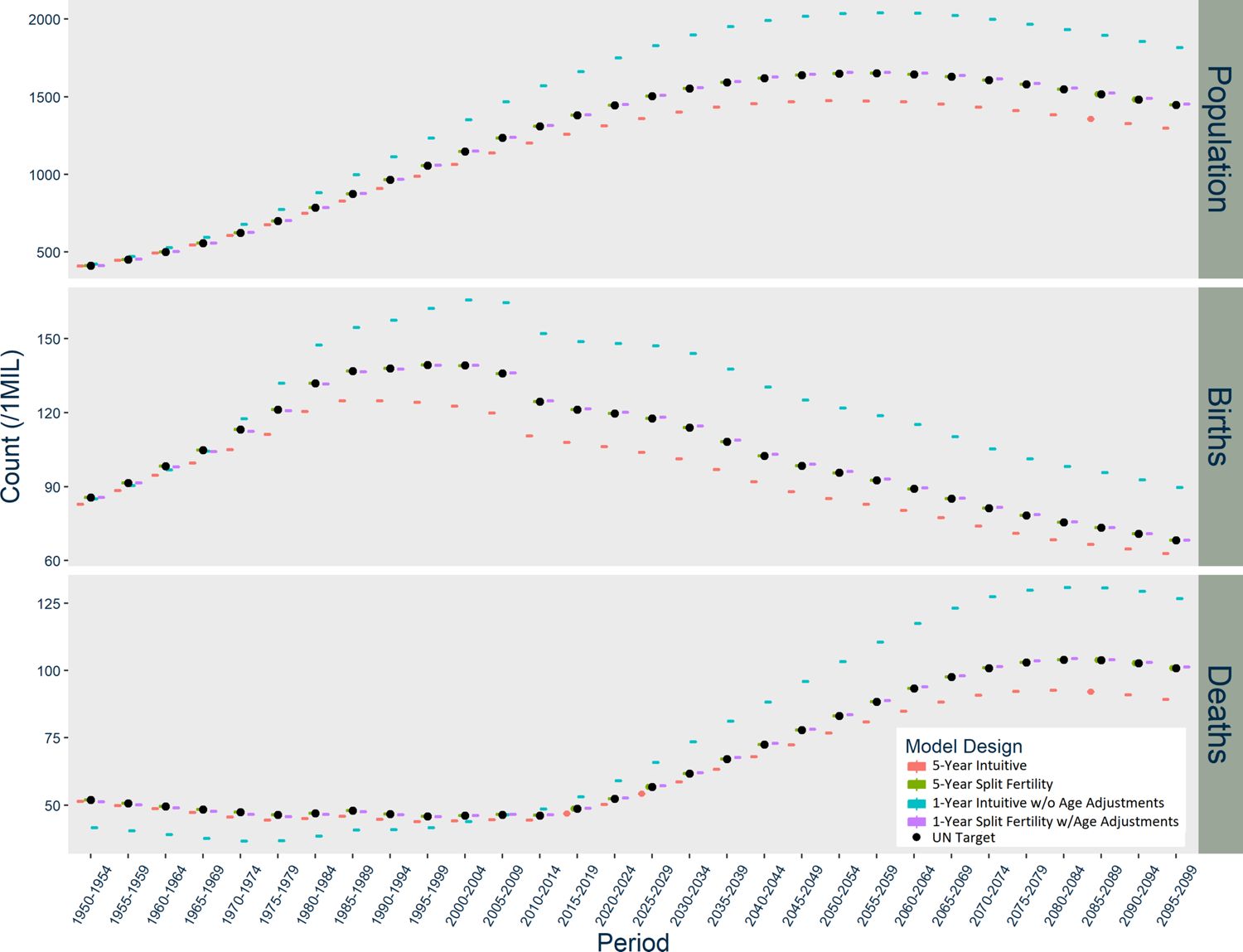
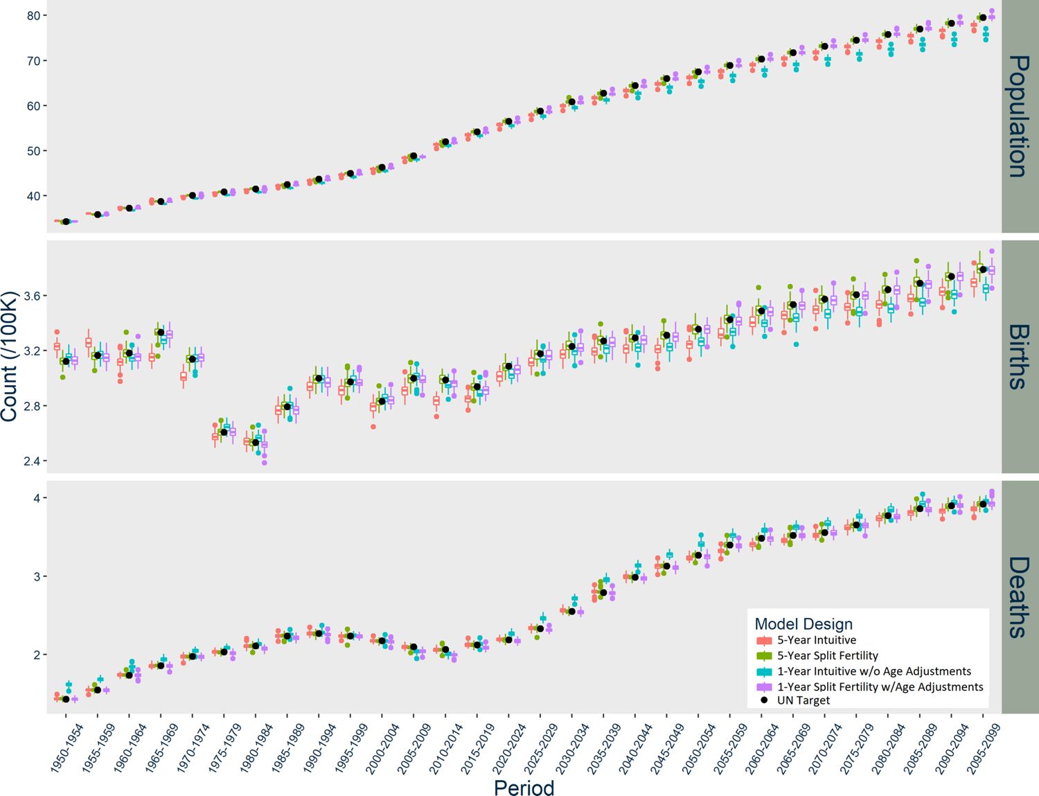
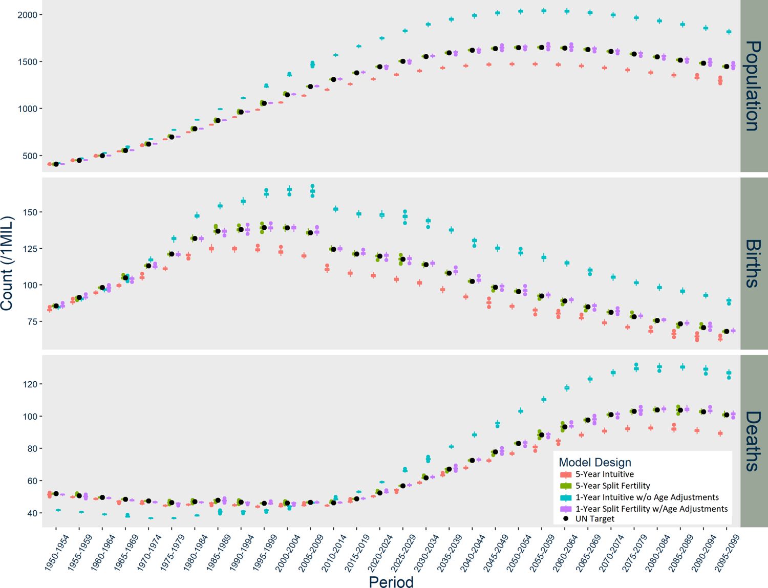
Figure 1–3 graph the results of each model for Norway, the US, and India respectively. In Norway (Figure 1), the five-year Intuitive design initially produces too many births, but then it consistently underestimates births. The one-year Intuitive design produces much smaller magnitude of divergence in births than the five-year model through 2050, but afterward there are fewer and fewer births than expected each period. The one-year Intuitive design produces particularly higher death counts than expected in 1950-1980 and after 2020. Taken together, the Intuitive designs’ divergences in births and deaths result in a slightly underestimated population size by 2100. In contrast, the five-year Split Fertility design is a perfect match to UN targets, but the one-year version still has some divergence, with a very slight underestimation of deaths.
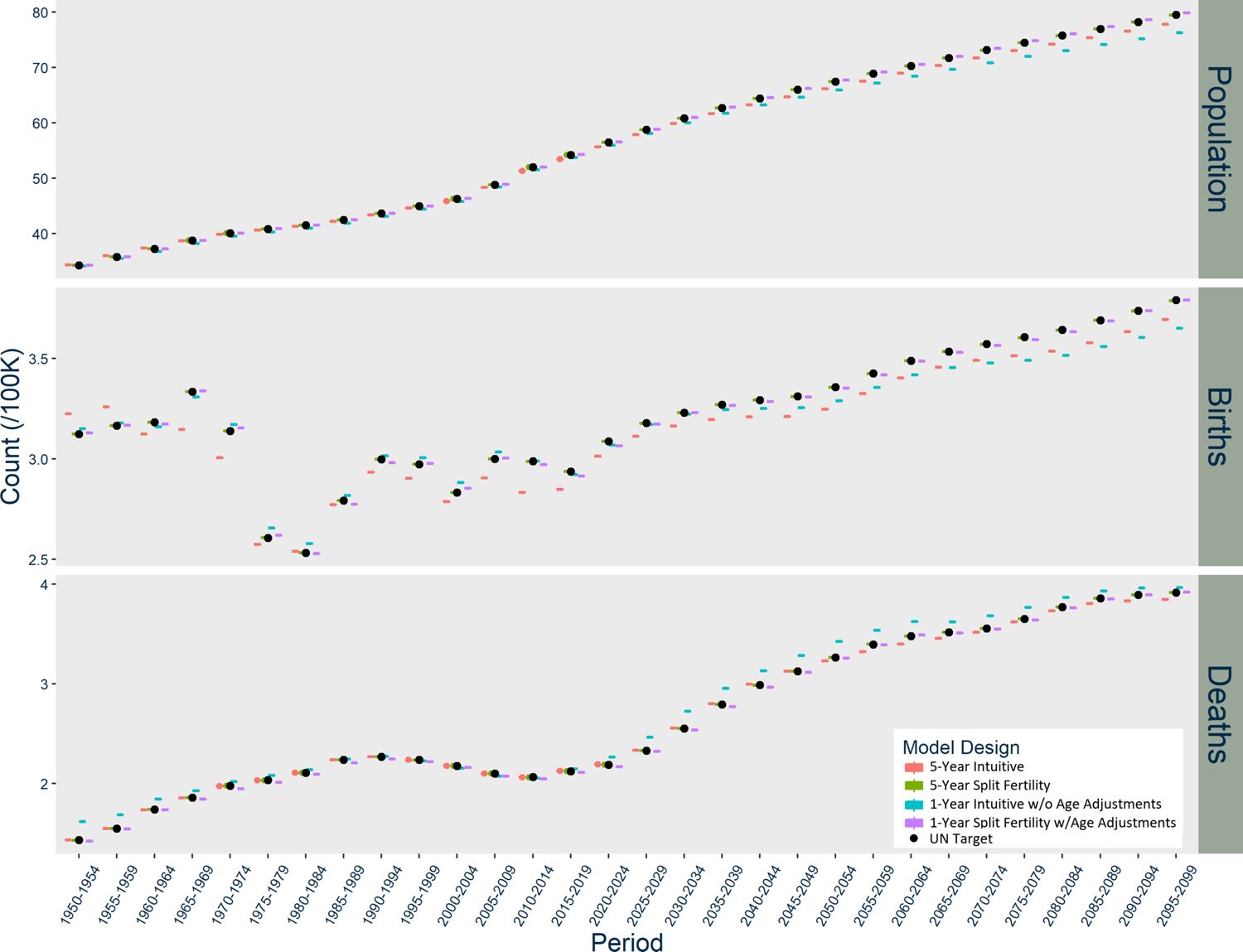
Results of Norway Models, scaled up to actual population size
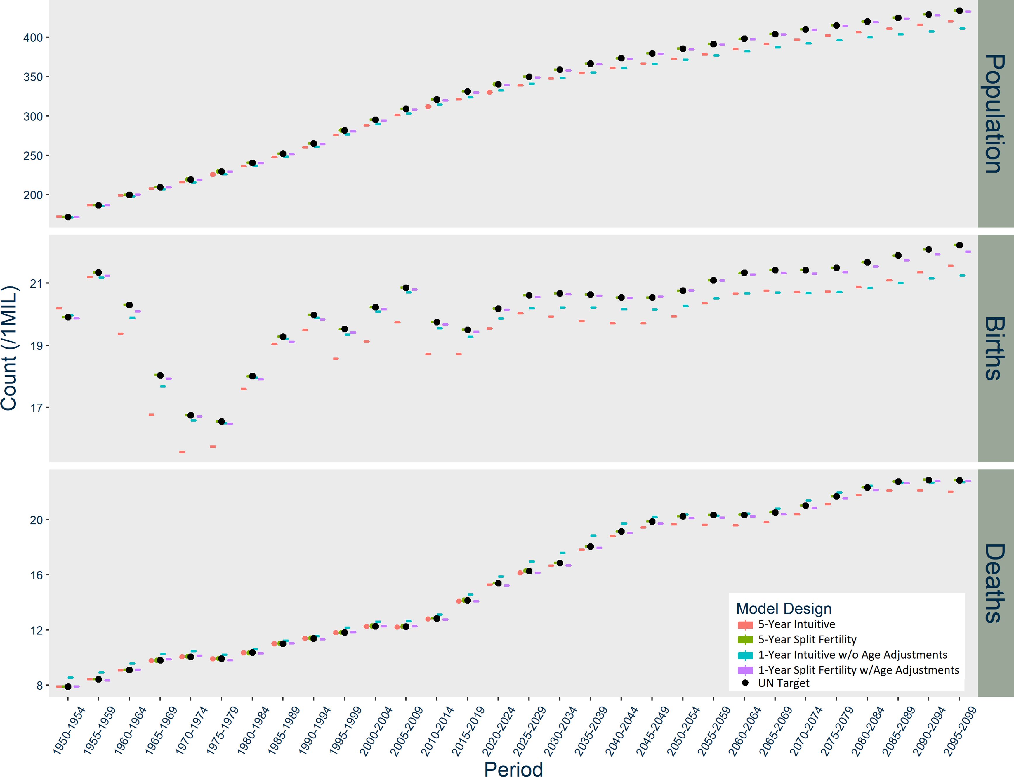
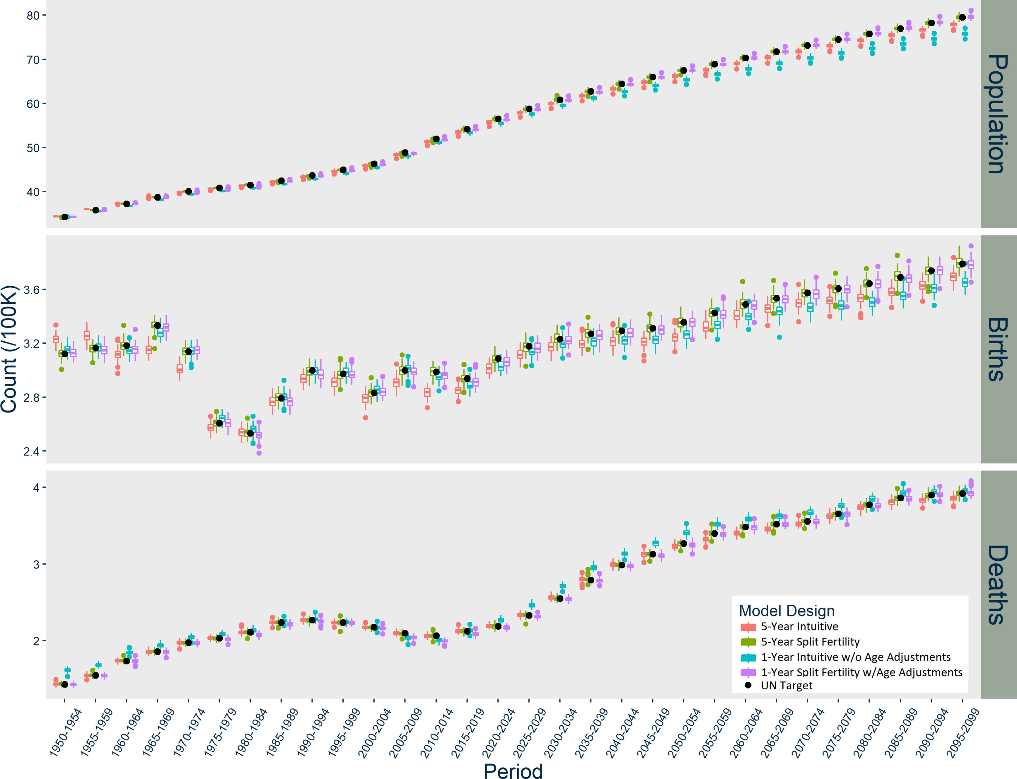
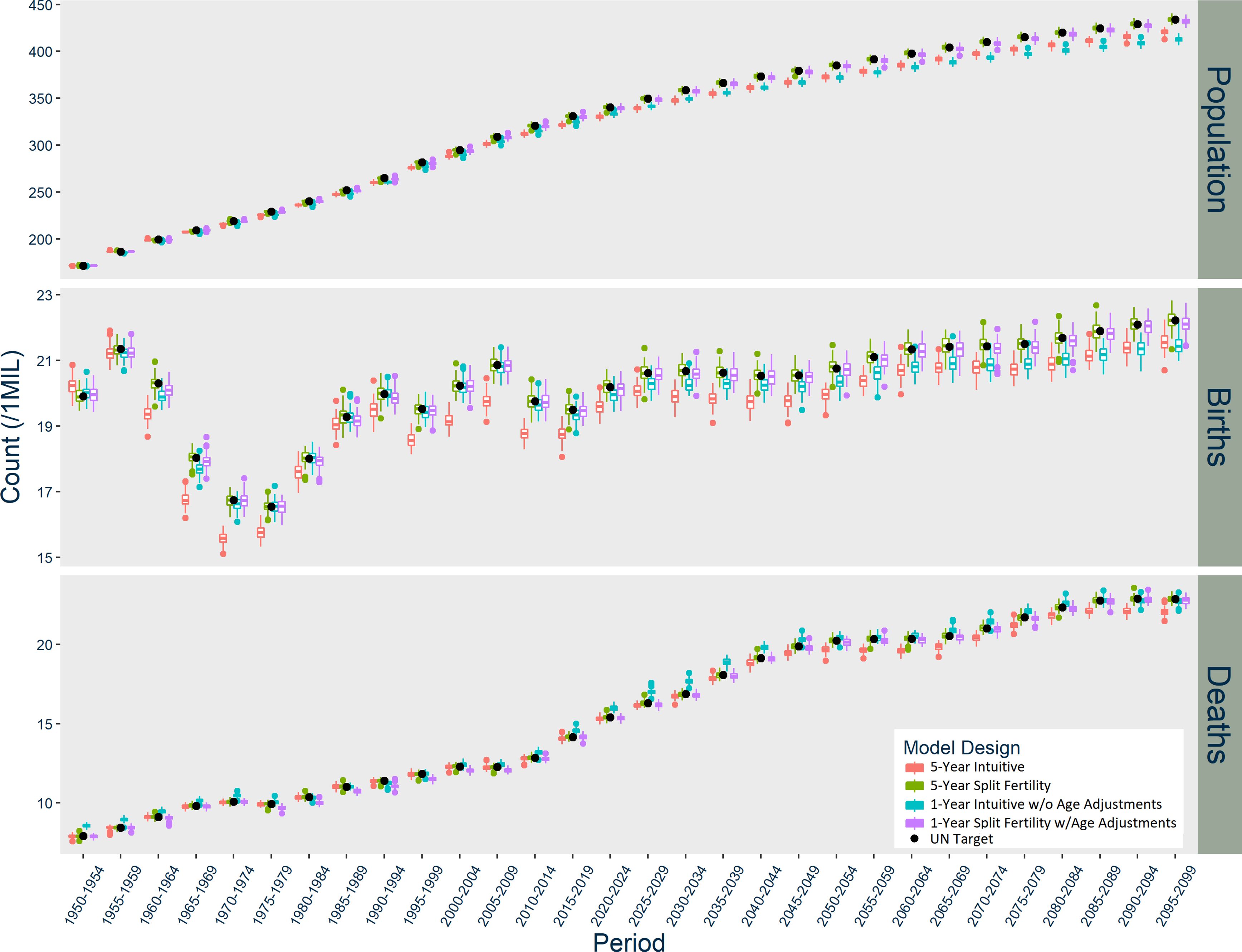
Results of USA Models, scaled up to actual population size
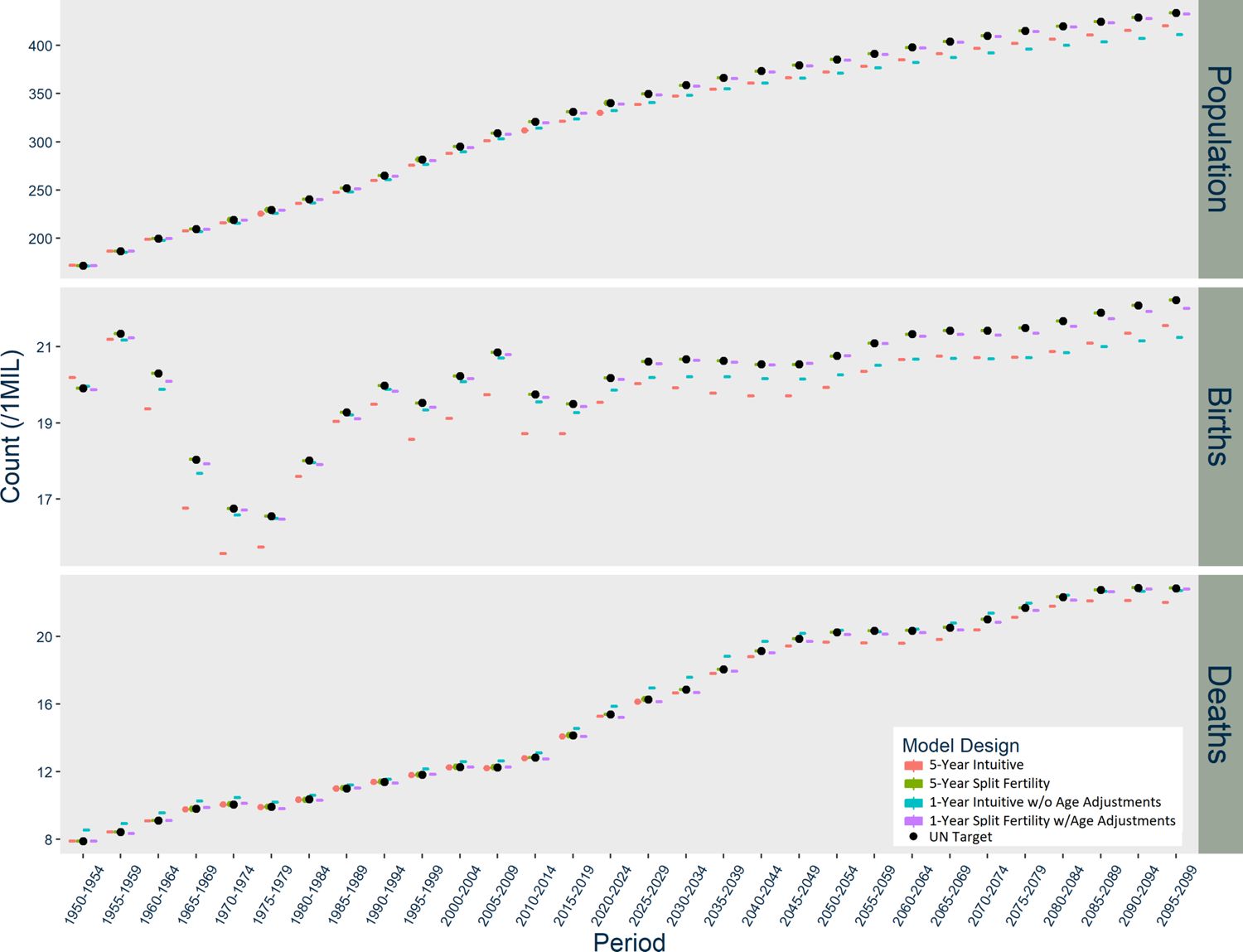
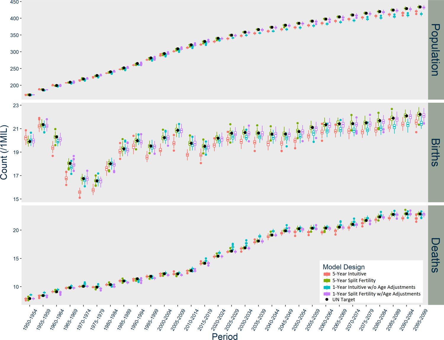
Results of India Models, scaled up to actual population size
The patterns of divergence for the US models (Figure 2) are similar to Norway, but of greater magnitude. The US Intuitive designs underestimate births in the first period, and the one-year Intuitive design likewise overestimates deaths during several periods. The USA five-year Intuitive design noticeably underestimates deaths after 2030. The Intuitive designs’ underestimation of the overall population in the US occurs earlier than in Norway. Meanwhile, the US five-year Split Fertility design yields an almost exact match with the UN’s estimates and projections, although the one-year version slightly underestimates births and deaths.
In India (Figure 3), the Intuitive designs produce opposite patterns of divergence, while the Split Fertility designs are both exceptional matches to UN targets. The five-year Intuitive model underestimates births, while the one-year version overestimates births starting in 1970. The five-year Intuitive design likewise underestimates deaths, particularly after 2030, while the one-year version initially underestimates deaths until 2005 when it dramatically overestimates them thereafter. Overall, the five-year Intuitive design underestimates total population and the one-year version overestimates it, but only after a few decades have passed.
6. Discussion
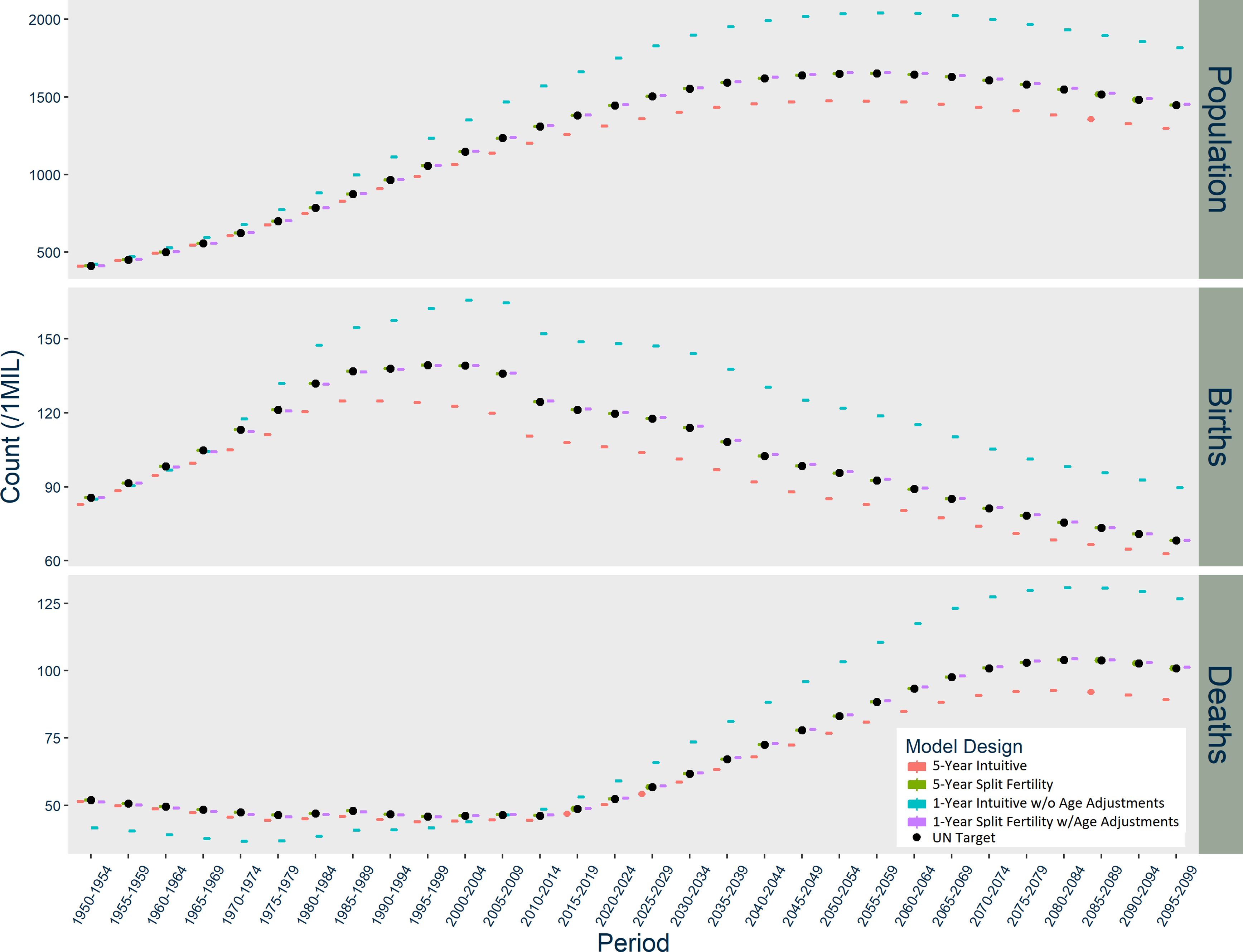
It is worth contemplating why the Intuitive designs diverge from the UN CCM projections in different ways across the three countries analyzed in the study. In Norway, the divergence is relatively negligible regardless of design; in the US, the Split Fertility design clearly benefits the estimation of births; and in India, the divergence becomes quite large with time and in different directions depending on the time-step of the model. The magnitude and specific pattern of the divergence varies because of population dynamics and potential compounding from trends among females of childbearing age. Figure 4 summarizes the population dynamics of each country among females age 15-49 based on UN data. India is going through the first demographic transition during the first 50 years of the simulation, which results in rapid population growth. The US and Norway are going into the second demographic transition, with low fertility, mortality, and an aging population, but they are also hosts to large waves of immigration that offset population decline.
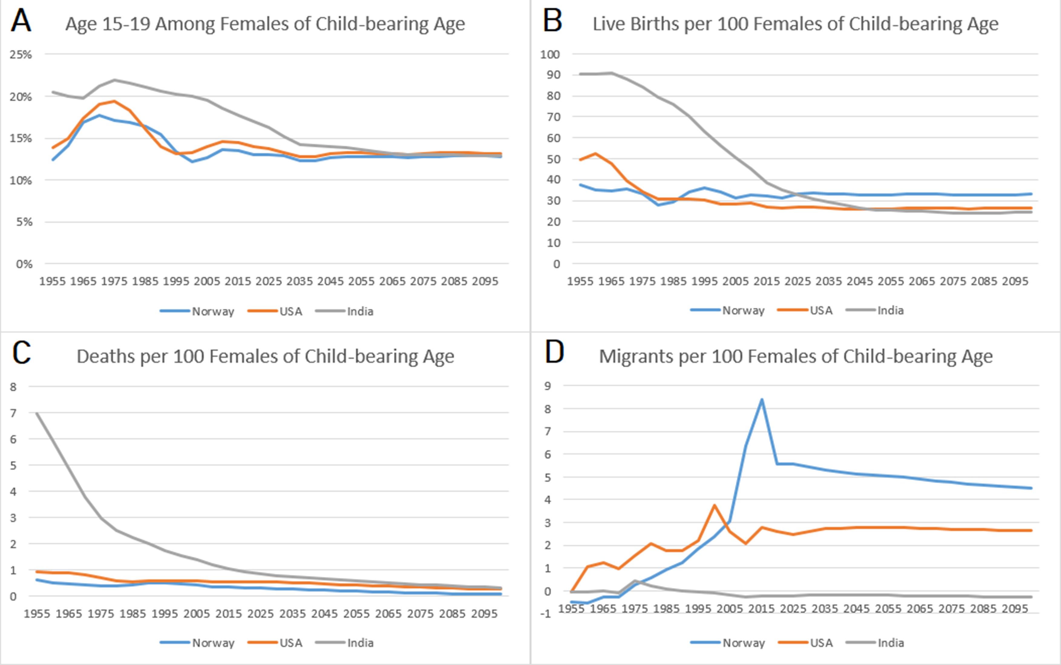
Population Dynamics Among Females of Child-bearing Ages (15-49), UN Data WPP2019
The five-year Intuitive design underestimates births in populations with growing female populations at childbearing age, overestimates births in populations that are declining, and the timing of this growth and decline produces unique patterns of divergence. Large divergence in births naturally has compounding consequences for deaths and total population. In the 1950s, there are excess births in Norway because the population of females at childbearing ages is declining from emigration and the consequences of low fertility during World War II. There are suddenly far fewer births than expected during the 1960s because the baby boomer cohorts age into childbearing risk, and then divergence diminishes in the 1970s as the age distribution becomes rectangular. Immigration to Norway increases, peaking between 2005 and 2015, and thereafter the Intuitive designs underestimate births. The US experiences similar patterns in age structure and immigration, but never has net emigration and has an earlier peak in immigration than Norway. The divergence in India’s five-year Intuitive designs seems negligible at first, because initially high mortality maintains a delicate balance in the size of rapidly growing female cohorts. The divergence in births picks up between 1960 and 2000, because the sharp decline in mortality permits rapid growth in cohorts at risk for childbirth. As the age structure becomes more rectangular, the divergence in births stabilizes. The underestimation of deaths becomes much larger in magnitude in the latter part of the 21st century, because the high-risk age groups are much smaller than anticipated by the UN statistics.
Population dynamics and compounding divergence also explain why the one-year version of the Intuitive design performs better than its five-year counterpart in Norway and the US to some extent, but does much worse in India. By itself, moving to a one-year step reduces divergence in births because it allows mortality, migration, and aging to occur each year before the subsequent year’s fertility. This minimizes compounding divergence in the US and Norway initially. Consistently high immigration in later decades, however, underestimates births further because the immigrants are all older than expected, which diminishes their contribution to fertility. India’s results in the one-year Intuitive design are almost entirely due to exceptionally high mortality in early years, which resulted in severe under-estimation of infant mortality. In subsequent decades, cohorts who aged into childbearing risk were much larger than expected and therefore larger cohorts are born thereafter. When all the exceptionally large cohorts become older, they are exposed to high death risk earlier than expected, which leads to much higher death counts than the UN targets.
Although the five-year and one-year Split Fertility designs perform well across country context, there is persistent divergence in the US and Norway one-year Split Fertility design. This occurs due to rounding error from the sorting method, because all events in a simulation result in discrete counts of affected agents, and rare events or events among small populations floor at zero (Bekkering, 1995; Van Imhoff and Post, 1998). This particularly affects migration events in the one-year model, because we divide total migrant counts in each age/sex group by 25, and the adjusted count must be an integer. Even with large net migration in Norway and the US, some age/sex groups will have too-few immigrants after dividing by 25, which leads to slightly too-few women of childbearing age. These errors could also affect events among small age/sex groups that have very low probability, such as fertility and mortality among some periods and age groups. These problems are minimal in India for two reasons: 1) High population growth leads to a very large population quickly despite all countries starting with 100,000 agents, 2) India experiences minimal net migration, which means that rounding errors in migration make almost no difference in observed outcomes.
The model designs presented here represent a series of adjustments and selection of options that are necessary to closely match UN population dynamics. We have demonstrated the implied ordering and assignment of risk by age dictated by the mathematical relationships within the UN’s CCM inputs and outputs, and the consequences for disregarding some of those relationships. Implementing these procedures in a simulation, which always operates prospectively and at the individual level, is far from intuitive. A common challenge in simulation research is integrating multiple data sources of varying quality and measurement assumptions (Müller, 2009; Riecke et al., 2019). Non-demographers frequently design simulations, and understanding a specific CCM is not a natural next step after downloading UN data. The Split Fertility design simplifies the process of implementing basic population dynamics in multiple countries and over many decades using the same standardized data source. Because the UN data are internally consistent, the Split Fertility design specified here minimizes the need for alignment procedures, which are popular and controversial course-correction methods in microsimulation (Li and O’Donoghue, 2014).
The Split Fertility design adapts a five-year standard CCM that is popular among demographic projection methods, which makes the design applicable to simulations that rely on non-UN CCM demographic statistics as well. It is important to recognize, however, that other design options are more appropriate when using different data sources or implementing other demographic processes within a simulation. A CCM designed for smaller geography, or for specific sub-groups of the population (e.g. ethnic groups), may operate with different statistics than the UN’s CCM (Birkin and Wu, 2012; Smith et al., 2013). Introducing additional demography modules (e.g. domestic migration), agent decision-making (e.g. partner selection), and social networks (e.g. kinship) further complicates how population dynamics are implemented. The DYNAMIS-POP microsimulation platform, for example, uses country-specific projection and microdata as inputs, and can incorporate modules on education, intergenerational transmission of ethnicity, partner selection, and prenatal care (Spielauer and Dupriez, 2019). The Split Fertility design is not a standalone microsimulation platform, but its data requirements and specifications make it an ideal demographic module for multi-country or comparative simulations.
It is also important to recognize that our analysis does not compare whether MSM or CCM approaches to population projection are superior. The Split Fertility MSM uses the same assumptions and inputs as the UN’s CCM. Using UN statistics as inputs means the simulation is accepting the UN’s assumptions concerning future trends in fertility, mortality, and migration. Not everyone agrees with those assumptions, and other projection assumptions are more appropriate for some projects (O’Neill et al., 2000; Roser, 2013). Even if using UN assumptions and data is appropriate, it may not be appropriate to use the Split Fertility design exactly as we specify in this paper. Alternative or adjusted designs may be more efficient, realistic, or meet the needs of the specific project without introducing significant divergence. For example, we also developed a design for Norway that operates in one-year steps and uses the crude mortality rate instead of the survival ratio, and still achieves low divergence (Puga-Gonzalez et al., 2022). We are currently testing a broader range of options to assess the consequences of selecting different combinations.
7. Conclusion
Demographic microsimulations are incredibly flexible in how they can incorporate different assumptions and complex processes that affect, and are affected by, population dynamics. This flexibility can become a burden when there is uncertainty about which options are most appropriate for a specific project. We identified a set of options necessary when using demographic statistics derived for standard CCM projections, but there are many data sources and statistics available. Knowledge of the relationship between demographic statistics and the population totals can inform simulation design. As demonstrated in this paper, harnessing the flexibility of simulations is a powerful tool for unveiling hidden assumptions when validating against an external standard.
The Split Fertility design works because it uses the event ordering implied by the UN’s CCM, approximates the mid-point population for fertility rates, and distinguishes between cohorts and age groups when assigning risk. It maintains minimal divergence over a 150-year span even when operating in one-year steps, which is highly desirable in simulation research where annual outcomes are common. The design is also appropriate for multiple countries of varying population size and dynamics, which makes it perfect for comparative simulation projects.
The future of simulation research is bright, and it is imperative that demography and population dynamics are a part of it. With growing complexity, temporal scale, and capacity, simulations can model real-life populations and contribute insights to a host of research questions in multiple fields. Moreover, simulations can do that with a degree of flexibility that is unmatched by traditional demographic projection methods, allowing demographers to exercise greater theory-grounded control over implementation assumptions. This places a responsibility on demographers at the forefront of simulation research to communicate the demographic principles, mathematical relationships, and assumptions present in simulation design.
Footnotes
1.
The 2019 WPP and previous UN revisions operate in 5-year intervals, but the most recent revision (2022 WPP) operates in 1-year intervals. CCMs that operate in 5-year intervals are still very common, which means our adaption of the 2019 WPP CCM may be generalizable to similar non-UN models. Future research can consider which additional adjustments are necessary when adapting a CCM operating in 1-year intervals.
2.
The UN estimates migration in ways other than the residual method, depending on data sources in each country. However, the survival ratio calculation operates under the assumptions of net migration as a residual, and using the survival ratios alongside net migration allows for standard interpretation across countries.
3.
We compared our calculation against age-specific counts graciously provided to us by the UN to confirm our approach was correct.
4.
For an in-depth discussion of demographic statistics, see Preston et al. (2000).
5.
While other similarly intuitive event-sequencing options exist (e.g. randomizing their order, assigning conditional probabilities, or moving aging to the last event), our Intuitive design is an efficient fixed order design that someone with a basic understanding of the UN’s CCM could implement quickly.
6.
In essentially all countries and periods, infant mortality is much higher than mortality for children aged 1-4.
7.
Tracking five-year cohorts to describe both starting and ending ages is also appropriate, but we have separated them here to be consistent with how the cohorts have different labels when used in the UN CCM.
8.
It is important to note that Table 2 differs from a traditional lexis diagram because it operates in whole years of risk. It is more accurate to assume average risk as halfway through the year, that is, each year column in Table 2 is split in half and cohorts are born halfway through the first year on average. Therefore, cohort “A” should have 4.5 years of total risk, because they only experience 0.5 years of risk in their first year. Similarly, cohort “E” would only have 0.5 years of risk. Altogether, newborn cohorts would have only 12.5 years of risk. However, this has consequences for the accuracy and simplicity of implementation in a simulation, particularly for migration. Dividing the migration count by another half introduces more rounding error because migration is relatively rare when the simulation population is scaled down. In the first year a cohort is born, there could be zero migrants to the cohort simply because halving the count does not result in an entire agent, and there will be five too few migrants in that interval. Net migration can be consistently underestimated and eventually impact other population dynamics if the problem persists over decades, which is the case for projection years (2020-2100) when net migration is held constant. One alternative is to calculate risk for each newborn cohort separately (e.g. cohort “A” annual proportion of net migrants is calculated as 4.5/12.5/5 multiplied by total expected newborn migrants, cohort “B” has 3.5/12.5/4, and so on), but this is needlessly complex. Another alternative is to introduce stochasticity, where a minimum number of migrants leave/arrive each time step and the fraction of expected migrants becomes the probability of an additional migrant for that time step. This option introduces complexity and variability. The difference in approaches is likely small. We believe our solution is the most straightforward way to recognize uneven risk among newborn cohorts while achieving both a good match to UN targets and simplicity in simulation design.
9.
Alternative calculations of mortality risk at smaller time intervals with higher accuracy are likely available, but we were unable to find a more accurate straightforward solution. Implementing more complex adjustments would have marginal return to accuracy for a microsimulation. Our estimate of infant mortality risk introduced very little divergence even in a country with high infant mortality, and the divergence is negligible in countries with low infant mortality.
10.
The UN provides limited annual and single age-group statistics as interpolated from their five-year data. We only use the one-year data to initialize the population in one-year age groups. The annual and individual age group data is insufficient to adapt the UN’s five-year CCM to a one-year model.
Appendix
Calculating Net Migration as a Residual in UN projections
These calculations are only necessary to get the age/sex distribution of migrants for the years 1950-2020 since net migration is the same as observed in 2015-2020 thereafter. In following UN procedures, net migration is only calculated for those aged 0-84. Calculations must be conducted independently of the previous or subsequent period to prevent compounding error from rounding. Follow the following procedure to calculate net migrants by age/sex:
Calculate mid-point population for female cohorts aged 15-49 by taking the simple average of populations in each cohort at the start of each period
Calculate number of births using formula: [Mid-period female pop*(ASFR/1000)*5]
Distribute births by sex using infant sex ratio
Apply Survival Ratios to determine survival of matching age group, with exception of the following:
Apply “0” survival ratio to the new infants
Apply “1” survival ratio to the 0-4 age group
Apply “95” survival ratio to those age 100+
Age forward everyone by 5 years (new infants are now in 0-4 age group)
Calculate net migration as the simple difference between the population size in each sex group for age groups 0-84, and the corresponding population at the start of the next period
Supplementary Stochastic Model Results
The models presented below use the same time steps, event ordering, assignment of risk, and changes to UN statistics used for the main results of the manuscript. We ran 100 iterations of each model design in each country, and the distributions are shown as boxplots (Figures A1–A3). Instead of using the sorting method to determine how many agents experience the demographic events, these models use individual experimentation. When fertility, mortality, and emigration events occur, an agent rolls a uniform distribution between 0 and 1, and experiences the event if their roll is less than the value of the UN statistic. This option is common in simulation design, and naturally introduces more variation in the number of births, deaths, and emigrations that occur at each time step. Fertility appears to have much higher variability than deaths and total population, but this is primarily a difference in scaling.
Results of Norway Models with Additional Stochasticity Options, scaled up to actual population size
Results of USA Models with Additional Stochasticity Options, scaled up to actual population size
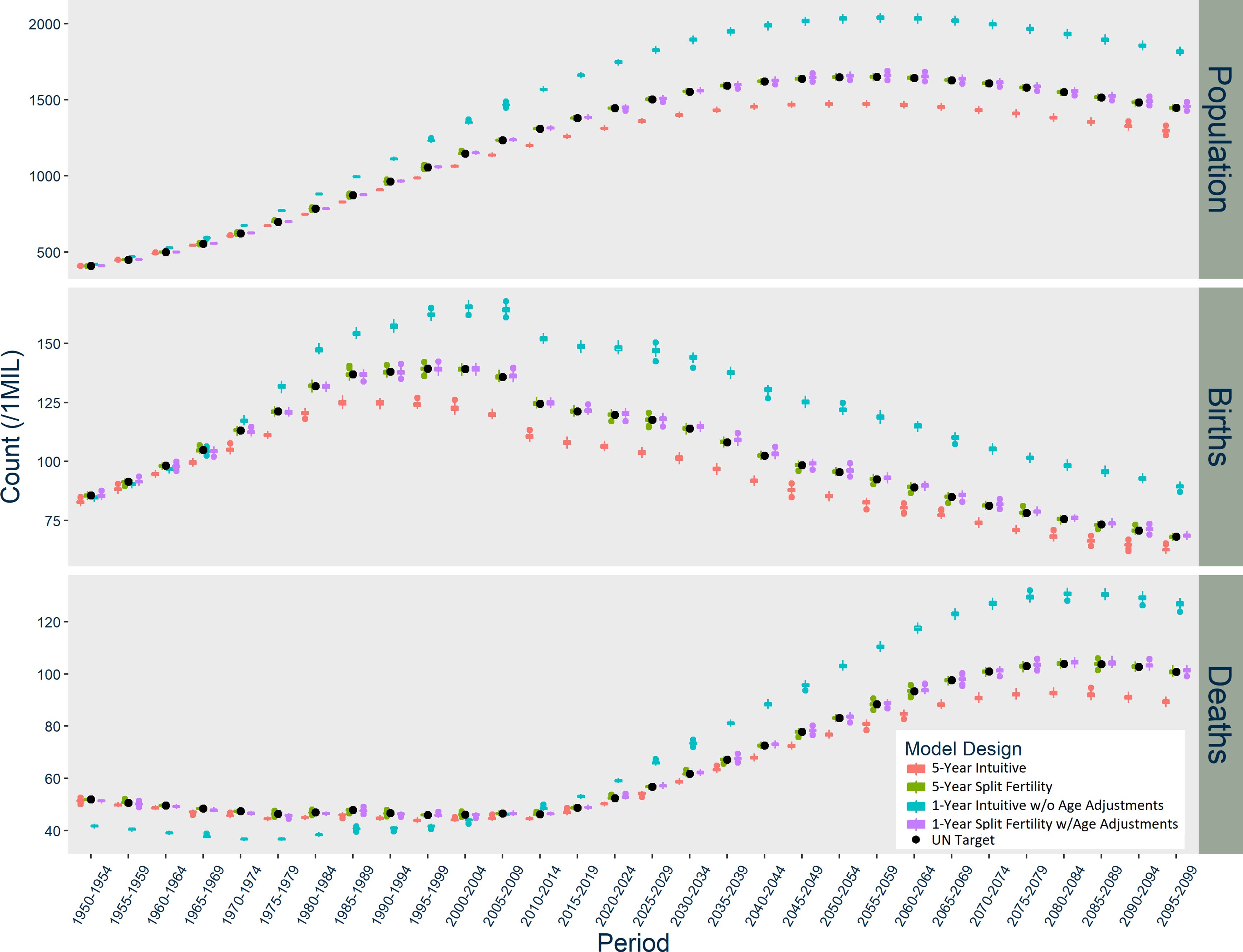
Results of India Models with Additional Stochasticity Options, scaled up to actual population size
References
-
1
Highlights of Contemporary MicrosimulationSocial Science Computer Review 29:3–8.https://doi.org/10.1177/0894439310370084
-
2
Combining Microsimulation and Agent-based Model for Micro-level Population DynamicsProcedia Computer Science 80:507–517.https://doi.org/10.1016/j.procs.2016.05.331
- 3
-
4
Agent-Based Models of Geographical Systems51–68, A Review of Microsimulation and Hybrid Agent-Based Approaches, Agent-Based Models of Geographical Systems, Springer Netherlands, p, 10.1007/978-90-481-8927-4.
- 5
-
6
Social and child care provision in kinship networks: An agent-based modelPLOS ONE 15:e0242779.https://doi.org/10.1371/journal.pone.0242779
-
7
A survey of dynamic microsimulation models: uses, model structure and methodologyInternational Journal of Microsimulation 6:3–55.https://doi.org/10.34196/ijm.00082
-
8
Evaluating Binary Alignment Methods in Microsimulation ModelsJournal of Artificial Societies and Social Simulation 17:15.https://doi.org/10.18564/jasss.2334
-
9
Microsimulation Population Projections with SAS: A Reference Guide25–49, Converting a Cohort Component Model into a Microsimulation Model, Microsimulation Population Projections with SAS: A Reference Guide, Springer International Publishing, p, 10.1007/978-3-030-79111-7.
-
10
In Handbook of Microsimulation ModellingDemographic models, In Handbook of Microsimulation Modelling, Emerald Group Publishing Limited, 10.1108/S0573-85552014293.
-
11
Modelling demographic changes using simulation: Supportive analyses for socioeconomic studiesSocio-Economic Planning Sciences 74:100938.https://doi.org/10.1016/j.seps.2020.100938
-
12
Demographic Modelling: The State of the ArtParis: INED. FP7-244557 Projet SustainCity.
- 13
-
14
Social Science Research NetworkSocial Science Research Network, 10.2139/ssrn.1465424.
- 15
-
16
Demography: Measuring and Modeling Population Processes. 2001Malden, MA: Blackwell Publishers.
-
17
Adapting Cohort-Component Methods to A Microsimulation: A case studySocial Science Computer Review 40:1054–1068.https://doi.org/10.1177/08944393221082685
-
18
Integrated population models: Model assumptions and inferenceMethods in Ecology and Evolution 10:1072–1082.https://doi.org/10.1111/2041-210X.13195
- 19
-
20
A Practitioner’s Guide to State and Local Population ProjectionsDordrecht: Springer.https://doi.org/10.1007/978-94-007-7551-0
-
21
What is Social Science Microsimulation?Social Science Computer Review 29:9–20.https://doi.org/10.1177/0894439310370085
-
22
A Portable Dynamic Microsimulation Model for Population, Education and Health Applications in Developing CountriesInternational Journal of Microsimulation 12:6–27.https://doi.org/10.34196/ijm.00205
-
23
The impact of demographic change in the balance between formal and informal old-age care in Spain. Results from a mixed microsimulation–agent-based modelAgeing and Society 42:588–613.https://doi.org/10.1017/S0144686X20001026
-
24
World Population Prospects 2019: Methodology of the United Nations Population Estimates and ProjectionsDepartment of Economic and Social Affairs, Population Devision.
-
25
Microsimulation Methods for Population Projection97–138, Microsimulation Methods for Population Projection, Population, An English Selection, p.
-
26
Microsimulation in demographic researchInternational Encyclopedia of Social and Behavioral Sciences 15:343–346.
-
27
Dynamic microsimulation models: A review and some lessons for SAGESimulating Social Policy in an Ageing Society (SAGE) Discussion Paper. 2.
Article and author information
Author details
Ivan Puga-Gonzalez

Funding
This work was supported by the John Templeton Foundation (Modeling Religious Change, #61074).
Acknowledgements
Patrick Gerland, PhD Chief of Population Estimates and Projections Section at the United Nations Population Division) confirmed the calculation and implementation procedures of the UN’s cohort component model. Anne Morse, PhD (Survey Statistician at the U.S. Census Bureau) provided early input and feedback on replicating cohort component model output. We also acknowledge support from the John Templeton Foundation grant #61074–note that the findings of this paper do not necessarily reflect the views of the John Templeton Foundation.
Publication history
- Version of Record published: December 31, 2023 (version 1)
Copyright
© 2023, Bacon et al.
This article is distributed under the terms of the Creative Commons Attribution License, which permits unrestricted use and redistribution provided that the original author and source are credited.