The Projected Development of the Gender Pension Gap in Switzerland: Introducing MIDAS_CH
- University of Liechtenstein, Liechtenstein, and Albert-Ludwigs-Universität Freiburg, Germany
- Federal Planning Bureau and CESO, KU Leuven, Belgium
Abstract
This study presents the newly developed dynamic cross-sectional microsimulation model MIDAS_CH, which is developed to assess the pension adequacy of the 1st and the mandatory part of the 2nd pillar pension systems. By simulating the entire life-spans of native and immigrating individuals we analyse the impact of the most recent pension reform, which increased the statutory retirement age (SRA) of women from 64 to 65. Furthermore, the impact of a reduction of the conversion rate in the 2nd pillar - which is a quite likely policy scenario – is also analysed. Our simulations suggest that the GPG would decline from 23.6% in 2020 to 21.6% in 2070. Although this decline appears to be marginal, there are signs of a catching-up process, especially among higher incomes. This catching-up process of women’s pensions may be driven by an increasing share of women having a tertiary educational attrition, which results in higher wages and higher activity rates. This leads to a reduction of the GPG in the upper income range. However, since labour market participation as well as the extent of part-time employment are positively correlated with the level of education, this would also lead to a larger variance in women’s lifetime earnings. The simulation of the policy scenarios suggests that an increase in the SRA of women increases their retirement income only marginal, whereas a reduction of the conversion rate from 6.8% to 5.2% would decrease the 2nd pillar pension income by 23.5%.
1. Introduction
The Gender Pension Gap (GPG) measures the relative difference between the retirement income of both women and men. In a general form, the GPG(l, x) can be written as ; usually l is the mean of the variable of interest, x, e.g. gross pension income, including survivors’ pensions of the 65+, though l(.) can be any measure of location. The GPG therefore reflects how much the pension benefit of women lags behind that of men.
The GPG is usually much higher than the gender pay gap,1 since the latter is a view at any moment in time, whereas the former is the result of how gender differences in in the prevalence of part-time work, unemployment, withdrawals from the labour market, and the gender pay gap cumulate over the working lives of men and women (; Bettio et al., 2013; Jolly, 2014, 37 and 50). These differences in earnings may be related to other gendered behaviour, such as the impact of parental leave on wages after return (e.g. Lequien, 2012; Thévenon and Solaz, 2013), sectoral segregation, and so forth. However, since pension insurance systems include redistributive elements, the relationship between lifetime earnings and pension income after retirement is far from linear (Kirn and Dekkers, 2022). Thus, the impact of gender-specific aspects on pension income depends in part on the design of the pension system.
In Switzerland, the GPG for the 65+ group fluctuates between 40.2% in 2008 and 30.9% in 2018 (European Commission, 2021a) and averages 33.6% between 2007 and 2019. Using data from SESAM,2 Fluder et al. (2016) find that women’s total pensions are 37 percent- or nearly 20,000 Swiss francs (henceforth CHF) per year lower than men’s pensions, which is roughly €20,510.3 However, as we will see in more detail later in this paper, the GPG varies dramatically with the pillar of the Swiss pension system.4 The 1st pillar pensions have a negligible GPG of just under 3 percent while 2nd pillar pensions have a GPG that exceeds 60 percent. The differences in the GPG of the respective pillars are due to the redistributive elements of the 1st pillar, which predominantly benefit women. In the 2nd and 3rd pillars, where pension entitlements are directly linked to contributions and thus to income, the differences are large and reflect gender differences in lifetime income. Kuhn (2020) reports that women’s pension entitlements in the 1st pillar are higher than men’s despite their lower lifetime income. However, men’s 2nd pillar entitlements are more than twice as high as women’s, as are 3rd pillar entitlements.
Measures of the current GPG, such as Fluder et al. (2016), Kuhn (2020), Kuhn et al. (2021) and the European Commission (2021), are retrospective since the gender pension gap observed among today’s retirees is shaped by labour market behaviour over the past decades. Since labour market participation of women has increased from 68% in 1991 to 79% in 2014 and in addition, part time work rates among active women have increased (Kuhn and Ravazzini, 2017), the question arises how the changing labour market participation of women will affect the GPG in the future.
Measures of future GPG simulated with static microsimulation models are valuable for assessing specific aspects, such as the impact of informal care on future pension income (Kirn and Thierbach, 2020), but do not incorporate dynamic aspects, such as changes in labour market participation at the extensive and intensive margins or migration.
This paper will present a newly-developed dynamic microsimulation (henceforth DMSM) model for Switzerland and use it to make projections of the Gender Pension Gap in 2070 for the cohort entering the labour market in 2018, as well as for immigrants entering and emigrants leaving the labour market afterwards. These projections will be as consistent as possible with official demographic and economic projections produced by various Swiss institutions, including the Swiss Federal Statistical Office (FSO). Furthermore, we will study how key parameters (such as the conversion rate) and the effect of these exogenous projections change the simulation results. This will allow us to assess how the GPG would develop if the statutory retirement age of women would increase, or if the conversion rate of the 2nd pillar pension income would be reduced.
Our study follows Bonnet et al. (2006), who use a DMSM to study the effects of pension reform on the GPG for a cohort of men and women in France. Their analysis is however limited to private-sector pensions, whereas this study includes both the 1st and 2nd pillars of the Swiss pension system. Halvorsen and Pedersen (2019) also use a microsimulation model to study the projected GPG of one cohort for the reformed Norwegian pension system. Kirn and Thierbach (2020)
Our study follows Bonnet et al. (2006), who use a DMSM to study the effects of pension reform on the GPG for a cohort of men and women in France. Their analysis is however limited to private-sector pensions, whereas this study includes both the 1st and 2nd pillars of the Swiss pension system. Halvorsen and Pedersen (2019) also use a microsimulation model to study the projected GPG of one cohort for the reformed Norwegian pension system Kirn and Thierbach (2020).
The study by Dekkers et al. (2022) is closely related to this paper. It presents a more general view on the same Swiss simulation results, however in a comparative context with simulation results from Belgium, Luxembourg, Slovenia and Portugal. This paper is complementary to theirs in that it focusses on the Swiss case, and presents the microsimulation model that was developed to this aim.
We contribute to this literature as we are the first to produce projected GPGs of the Swiss Pension system, which provides a gender-specific perspective on how the design of the Swiss pension system might affect within- and between-gender inequalities of pension income in a context of net-immigration and demographic ageing. Furthermore, we extend the analysis from the gap measured at the mean, to gaps in the lower and upper ends of the income distribution. Our analysis concentrates on one birth-cohort – individuals born in 2000 – and we focus on two perspectives. First, we project the future GPG by mapping our own projections about the future labour market participation at the extensive and intensive margin. In a second step, we simulate the impact of the most recent pension reform, which increased the statutory retirement age (SRA) of women from 64 to 65. Third, we simulate the impact of a reduction of the conversion rate in the 2nd pillar - which is a quite likely policy scenario – and analyse its impact on the future GPG.
An important caveat is that our analysis is limited to the 1st pillar of the Swiss pension system and the mandatory part of the 2nd pillar. This means that the voluntary and more defined-contribution parts of the pension system are not included. The reason for this is the theoretical and empirical difficulty in the modelling of private savings (Tedeschi et al., 2013) and the trade-off with social security in dynamic microsimulation modelling (Rein and Turner, 2001). This would bring us too far from the ambitions of the paper, but it also means that we probably underestimate the GPG in both 2018 and in our projections.
The remainder of the article is organized as follows. The next section introduces the dynamic microsimulation model MIDAS_CH and puts it in the classification of existing models. This discussion will include the data used as the starting dataset as well as the auxiliary information and the alignment methods by which this is done. Section 3 describes in more detail the simulation of lifetime events in the field of demographics (birth, death, migration, etc.), labour market states, retirement and disability, as well as immigration and emigration. Section 4 provides information about the Swiss pension system and the simulation of pension income of 1st and 2nd pillar pension income. Finally, section 5 will present the simulation results of the model and discuss various projected gender pension gaps, in the base variant and the policy scenarios. Finally, we draw a conclusion and provide an outlook to the next steps in the development of the model.
2. The dynamic simulation model MIDAS_CH
MIDAS_CH (which is an acronym for ‘Microsimulation for the Development of Adequacy and Sustainability’) is a discrete-time DMSM using dynamic cross-sectional ageing. It is developed to simulate the distribution of pension income, and its underlying processes, including labour supply, migration, family formation and dissolution, and many others. As such, the model creates a synthetic panel dataset out of a cross-sectional observed starting dataset, by simulating the life spans of the existing individuals and their households while adding new-borns and immigrants, and removing emigrants and deceased individuals. Older – and further developed – models of the same group include MIDAS_BE in Belgium, MOSART in Norway, SESIM in Sweden, DESTINIE in France, T-DYMM in Italy and CBOLT in the US (see Li et al., 2014, for a discussion).
MIDAS_CH belongs to the MIDAS group of DMSM, which also includes models in Belgium, Luxembourg, Portugal and Hungary. It has taken the MIDAS_BE model as an example and source of inspiration (Dekkers et al., 2009; Dekkers and Van Den Bosch, 2016) and runs on LIAM2 (De Menten et al., 2014). In doing so, MIDAS_CH has benefitted considerably from the years of knowledge and experience of other users and developers of models in the MIDAS group (Bryon et al., 2018; Bryon et al., 2018; Dekkers et al., 2022; Dekkers and Van den Bosch, 2021; Li et al., 2014; Liégeois, 2021 Moreira and Wall, 2021Moreira and Wall, 2021), as have the other models in this list.
MIDAS_CH is set up as a discrete-time, cross-sectional ageing model, thereby allowing for the modelling of interactions between individuals, as between partners. This is relevant for the modelling of survivors’ benefits.
As the model follows a closed population approach, partners in the family formation process are selected sporadically from individuals in the dataset. Furthermore, following Dekkers (2015), individuals are cloned in the case of immigration, and removed from the sample in the case of death or emigration. Finally, discrete time models are easier to implement in stepwise computer simulations and often require fewer variables than continuous-time models (Li et al., 2014). But the main advantage of the combination of cross-sectional aging and discrete time simulation is that it allows to define exogenous constraints on the number of objects or events within each time unit, which assures, that the simulation results are consistent with exogenous projections and assumptions (Andreassen et al., 2020; Dekkers et al., 2009). This is explained in the next section.
2.1 Simulation and alignment
The purpose of a DMSM like MIDAS_CH is to produce long-term projections of pensions. As these pensions in some shape or form are the result of previous earnings or labour market participation, or even of the person being present in the country, this requires the simulation of the intertemporal development of a large variety of characteristics, such as demographic ageing, the household size and marital states, activity rates, etc. In its simplest form, this is mostly done using separate discrete-dependent variable models, such as logistic regressions. However, if these estimated models are considered sub-optimal,5 or if the researcher wishes to make use of projections that were developed by others in order not to reinvent the wheel and to paint a consistent picture, many models make use of so-called alignment techniques. Various alignment methods have been developed (Morrison, 2006), but Li et al. (2014); Li and O’Donoghue (2014) conclude that, for those simulation models that focus on the impact on distributions, the sidewalk hybrid and the SBDL6 methods achieve the best results. However, as sidewalk hybrid methods have a low computing performance, the “alignment by sorting” by the SBDL method is widely used in complex microsimulation models, and MIDAS_CH is no exception.
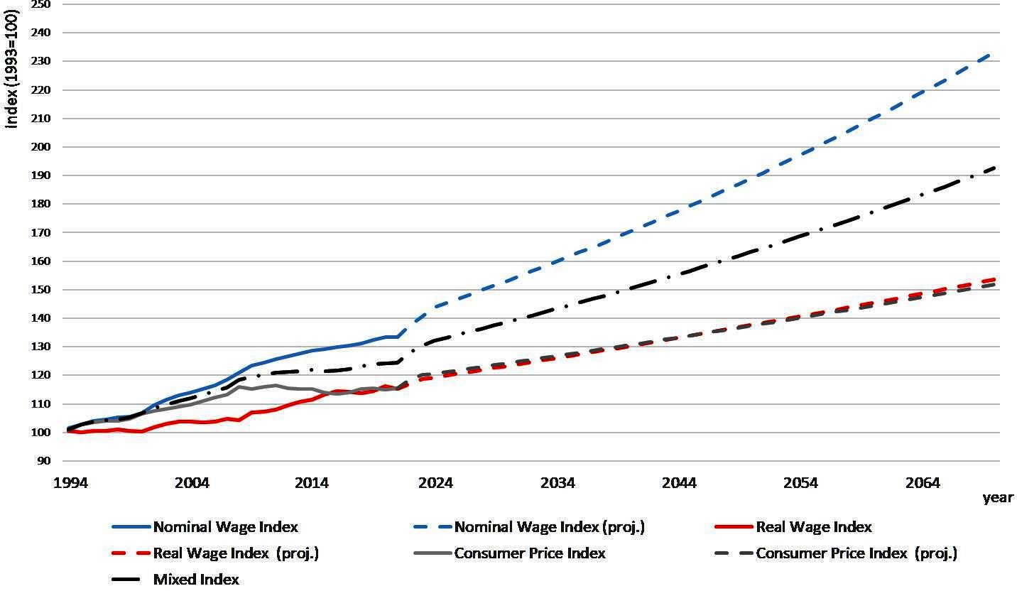
In addition to the alignment of the states, consistency with exogenous macroeconomic forecasts is achieved through the indexation of earnings and the adjustment of macroeconomic variables. In so doing, the simulated micro-level earnings are adjusted to be equal to macroeconomic wage growth projections. Furthermore, the minimum 1st pillar pensions and the related thresholds of the 1st and 2nd pillar pension are adjusted by the arithmetic mean of the consumer price index and nominal wage index (the so-called mixed index). The short-term forecast of the wage-price index is based on the estimate of SECO (2022). In the absence of official estimates of long-term future wage and price indices, it is assumed that future nominal wage growth rates would correspond to the average annual growth rates of the past twenty years, based on the nominal wage index (FSO, 2022b) and that the real wage growth is equal to the inflation rate (full inflation compensation). Figure 1 illustrates the nominal and real wage indexes based on official statistics (base=1993), as well as the projected nominal and real wage indexes, and the related consumer price index7 and mixed index.

Nominal and real wage index, consumer price index, and mixed index (base 1993). Source: FSO (2022b), own projections.
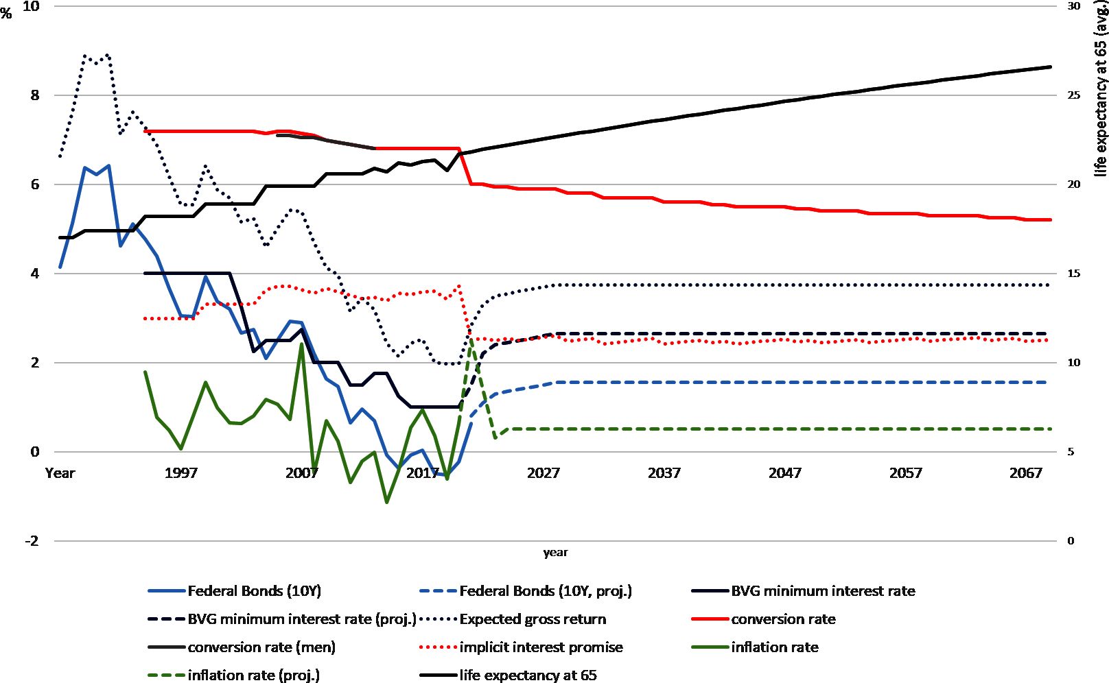
Additionally, a range of interest rates are projected, as these affect the central parameters of the 2nd pillar (see Figure 2). Based on the current inflation trend, it is assumed that the Central Bank rate will rise in the coming years (KOF, 2022), which will also result in an increase in the yield on 10-year federal bonds,8 as well as a decline in inflation rates. Accordingly, the expected gross return on pension wealth will increase, as in accordance with Art. 3 of Professional Guideline 4 (FRP 4), the upper limit is calculated as the interest rate of the 10-year federal bonds, increased by a surcharge of 2.5%9 and reduced by a discount (at least 0.3% -points) for the increase in longevity. Additionally, the minimum interest rate on accumulated assets of the 2nd pillar, which is set by the Federal Council according to the recommendation of the Federal Commission for Occupational Pensions, is adjusted according to our own forecasts on the return on federal bonds, as well as the expected gross returns. Hence, the yield on 10-year federal bonds and the expected gross return delimits the interest corridor on accumulated pension assets.

Actual and projected rates of return and life expectancy (at age of 65). Source: FSO (2022b), own projections.
Another key parameter of the 2nd pillar pension system is the conversion rate, which is the percentage at which an insured person’s retirement assets are converted into a life annuity. Since the conversion rate depends on the interest rate levels and life expectancy, assuming increasing life expectancies and low interest rates, a lower conversion rate is likely in the future. Based on a life expectancy at age of 65, which is projected by the FSO (2022c), the conversion rate is adjusted according to the annuity formula10 to achieve an implicit interest pledge, which is close to the minimum interest rate on accumulated assets of the 2nd pillar. Since widows' and orphans' pensions are not taken into account in this simplified approach, the resulting implicit interest rate tends to be underestimated.11 However, since the projected conversion rate is estimated using the minimum interest rate, which represents the lower boundary of the interest corridor on accumulated pension assets, the assumption is plausible. Thus, the estimated future conversion rate is 5.2%, which corresponds to the average conversion rate for the supplementary second pillar pension (currently 5.28%) for retirements in five years (OAK, 2021) seems plausible.
However, since a reduction in the conversion rate leads to a significant reduction of the pension income of the 2nd pillar (For example, a reduction of the conversion factor from currently 6.8% to 5.2% would reduce pension income by 23.5%),12 two different scenarios are simulated: 1) the conversion rate remains at today’s level, 2) the conversion rate will be lowered in the future. As a reduction in the conversion rate lowers the relative share of 2nd pillar pension income in total pension income, we also expect that this affects the simulated GPG, since the GPG is largely based on the gender differences in the 2nd pension pillar.
2.2 Database
As explained in previous sections, a discrete-time DMSM essentially creates a synthetic micro panel dataset out of a cross-sectional observed starting dataset. So the starting dataset is a crucial element of any model. MIDAS_CH is based on the Swiss SILC dataset of 2018, which is conducted by the Swiss FSO and represents the Swiss population. The Swiss SILC dataset has a sample size of 6,680 households, and approximately 15,200 individuals (FSO, 2018). Leaving out the 949 individuals in households for which no information was available, a balanced panel comprising 14,251 individuals and 6,263 households was used for the simulations. SILC datasets are widely used as database for arithmetic microsimulation models, like Euromod, as are some dynamic microsimulation models (Dekkers and Van Den Bosch, 2016; Li et al., 2014) due to their wide range of socio-demographic variables at individual and household level, as well as their international comparability.
Although the SILC dataset is a good data source to simulate life courses and pension income, some limitations of the database need to be mentioned. The survey uses the permanent resident population in private households as the primary population and survey unit. This includes persons without permanent residence who live together with at least one other permanent resident due to their living circumstances. However, the SILC data excludes people living in collective households, notably older people in care homes. As these persons consist mainly of the oldest men and women, this may affect the simulation results (Peeters et al., 2013).
Furthermore, the SILC does not contain information on the upbuilding of pension claims based on previous earnings of the currently active population. The earnings history cannot be derived from previous waves of the panel either, since the Swiss SILC, like all SILC datasets, is organized as a rotating panel with a panel duration of only four years. Nor are previous earnings histories available, so that the simulation of this actual implicit pension claim is not possible. Including this information on current pension upbuilding is a key ambition for the next version of MIDAS_CH, because it for now limits the simulation results to the first cohort that can be assumed not to have an implicit pension claim in 2018. This of course is the cohort that enters the labour market in 2018, and which will receive their pensions from 2062 onwards. So, for now, we need to limit our simulations to this cohort.
2.3 Dynamic weighting
Like most datasets, the SILC data for Switzerland includes weights to compensate for over- or under-sampling of specific cases, and for disproportionate stratification or to adjust for survey non-response (Verma et al., 2007). Frequency weights therefore have also to be applied in DMSM in order to obtain unbiased results.
In order to set up an efficient and accurate DMSM, various approaches exist. A first and simple approach is to expand the starting dataset using the frequency weights, and then take a sample from the expanded dataset (Dekkers and Cumpston, 2012). This approach is simple and straightforward but can result in loss of information, especially if the original dataset is comparatively small. The modelling approach (Galler, 1987, p. 313) and the shared weights approach (Ernst, 1989) are alternative approaches. These techniques can be used to determine the frequency weights (Schonlau et al., 2013). The modelling approach is used for the panels HILDA13 and SOEP14 to estimate the unknown selection probabilities of new households based on a model from the known probabilities and using the inverse selection probabilities as weights (see Haisken-DeNew and Frick, 2005; Watson, 2012, for a discussion). Finally, the shared weights approach, redistributes the frequency weight of a household equally among the household members. If, for example, two individuals from two households with different frequency weights form a new household, the individual weights are summed up and divided equally among the household members of the newly formed household. In this way, the shared weights approach keeps the total of individual weights within a household constant and redistributes the weights among the household members as new individuals enter a household. The shared weights approach is, for example, used in the household panels EU-SILC (Verma et al., 2007), PSID15 (Heeringa et al., 2011), BHPS,16 SLID17 (LaRoche, 2003).
As however the weighted objects have to be aligned with exogenous constraints, such as projected demographic developments, the interaction of alignment and weighting procedures has to be taken into account to avoid simulation errors. Dekkers and Cumpston (2012) propose three strategies to cope with the interaction of weighting and alignment. First, to split up the last household, second to select a household for alignment to give the lowest possible mismatch, third, to carry forward any misalignment to the next period. They tested these strategies and concluded that the third strategy is the most efficient in terms of runtime and memory requirements. In order to set up an efficient and accurate DMSM, in MIDAS_CH shared weights approach is implemented in combination with the carry forward of any misalignment, as proposed by Dekkers and Cumpston (2012).
3. Simulation of life events
Life events, such as becoming a parent, reducing work to care for relatives, unemployment and divorce, all affect pension upbuilding. For example, periods spent upraising and caring for children are credited in the 1st pillar pension scheme, but not in the other pillars. Other life events, such as unemployment or interruptions and reductions in employment, affect pension income through their impact on earnings. As is standard in a discrete time model, the likelihood that a given event will take place is simulated for every individual in each period.
The simulation of demographic events in MIDAS_CH uses the SDBL method (see section 2.1). To ensure that the simulated population structure stays as close as possible to the population structure projected by the FSO (FSO, 2017; FSO, 2020c), the simulation results are aligned to the official projections. But also other relevant official projections on household formation and dissolution; labour market participation -, unemployment -, and care-giving rates; part-time work rates; earnings growth rates, etc. are being taken into account in the simulations of MIDAS_CH. Table 1 provides an overview of the data sources used for the alignment.
Sources used for the alignment process
| alignment | source | data | dimensions | age groups | scenario variants |
|---|---|---|---|---|---|
| mortality | FSO | BEVNAT, ESPOP, STATPOP | gender | year | scenario A-00-2020 |
| births | FSO | BEVNAT, ESPOP, STATPOP | female | year | scenario A-00-2020 |
| population | FSO | BEVNAT, ESPOP, STATPOP | gender | 5-year brackets | scenario A-00-2020 |
| fertility | FSO | BEVNAT, ESPOP, STATPOP | female | year | scenario A-00-2020 |
| marriage | FSO | BEVNAT | gender, civil state | 5-year brackets | |
| divorce | FSO | BEVNAT | gender | 5-year brackets | |
| disability | FSO | IV | gender | 5-year brackets | |
| care | FSO | SGB | gender | year | |
| care giving | FSO | SGB | gender | year | |
| early retirement | FSO | NRS | gender | year | |
| labour market participation | FSO | SAKE | gender | year | |
| part-time | FSO | SAKE | gender | 5-year brackets | 3 categories of PT work |
| unemployment | FSO | SAKE | gender | 5-year brackets | |
| immigration | FSO | STATPOP | gender, nationality | year | scenario A-00-2020 |
| emigration | FSO | STATPOP | gender, nationality | year | scenario A-00-2020 |
-
BEVNAT = Statistik der natürlichen Bevölkerungsbewegung; ESPOP = Statistik des jährlichen Bevölkerungsstandes; STATPOP = Statistik der Bevölkerung und der Haushalte; SAKE = Schweizerische Arbeitskräfteerhebung; IV = IV-Statistik; NRS = Neurentenstatistik; SGB = Schweizerische Gesundheitsbefragung;
The next sections provide an overview of the modelling of demographic events as well as labour market participation and labour supply.
3.1 Fertility and mortality
In 1964, the total fertility rate (TFR) in Switzerland was 2.7 children per woman. But during the economic crisis in the 1970s, the birth rate fell drastically and has been below the replacement level ever since. Since 2009, the fertility rate has been around 1.5 children per woman. The TFR of Swiss and foreign national mothers born in Switzerland are very similar, but that of women born abroad is higher (FSO, 2020d; Guarin Rojas et al., 2018). Differences in fertility are determined by educational level since a longer period of education leads to a postponement of family formation (Van et al., 2015), and the opportunity costs of career interruptions are higher (Gustafsson, 2001). Most children are born within marriages, though the number of non-marital births has increased more than fivefold since 1970. These non-marital births are mostly the children of single women, most of whom live in a consensual partnership (FSO, 2020d). Hence, within the SDBL alignment method, the a priori probability of giving birth is simulated on the basis of a logistic regression model using age, educational attainment level, cohabitation and marriage as well as the number of siblings as arguments.
Currently, life expectancy at birth in Switzerland is one of the highest in the world, mainly due to the sharp increase during the 20th century. Average life expectancy at birth for men (women) was 81.9 (85.9) in 2019. In line with this trend, the remaining life expectancy at age 65 also increased significantly. The projections of the FSO assume that this increase in life expectancy will continue in the future. For example, the expected average remaining life expectancy of men and women at 65 born in 1952 (who turned 65 in 2017) will be nearly 21 and nearly 25 years, respectively, and increasing to 28 and 30 years for those born in 2017 (FSO, 2020c). To reflect the increased life expectancy in MIDAS_CH, the projected probabilities of death for men and women by age have been used as alignment information in the modelling of mortality risks.
3.2 Marriage and divorce
As mentioned above, MIDAS_CH is a closed model. Therefore, for each candidate for marriage, a stable marriage market algorithm available in LIAM2 is used to match potential spouses available in the dataset (Bryon et al., 2018). A first step in this procedure is the selection of potential candidates for marriage. Then women candidates are ranked based on how difficult they are to match, and the most difficult are then matched first. This “order of decreasing differences algorithm” prevents strange matches among the “last” people to be selected for marriage (Bouffard et al., 2001; Dekkers et al., 2009). It is not unusual for the ranking of each woman to be based on the difference between her age and the average age of the male candidates. In a third step, a matrix is constructed where for each woman, all male candidates are assigned a score that represents the assumed or observed likelihood of the match. In our model, this score is based on the age of the male candidate, the difference between the age of the man and woman, and the work status of the potential partners. In the final step, for each female candidate and in the order explained above, the male candidate with the highest score is selected from the vector of available men. Finally, an “alignment by sorting” approach is applied, whereas the cases of “actual marriages” are aligned with the projected figures (Dekkers et al., 2009).
The modelling of divorce is comparatively simpler. The probability of divorce is simulated for one partner in each couple; this probability is based on the results of a logistic regression of divorce on the base of the number of children, the duration of marriage, the age difference between the spouses, and combinations of work status of both spouses. This logit is combined with alignment using projections from the FSO.
3.3 Disability and informal care
The disability rate is closely related to age. While in 2020 less than 2% of the total resident population under the age of 30 received a disability pension, this share was 11.4% for men and 9.6% for women shortly before they reached the statutory retirement age (FSO, 2022b). When modelling disability, the probability of becoming disabled is estimated for each individual each year, depending on age, civil state and an interaction variable of age and education, before the alignment by sorting is applied according to the projected prevalence of disability by gender and age group. In the absence of official projections of disability prevalence, projected disability prevalence is assumed to follow the trend of recent years, but to begin to stabilize after 2040.
The next step is to simulate the need for informal care. In 2017, 13% of the population received help from relatives, acquaintances, or neighbours for health reasons. This percentage, which is higher among women, increases sharply from the age of 75. The proportion of people providing unpaid care is highest among those aged 45 to 64 (FSO, 2020a). Hence, the probability of need for care is simulated for each person each year, depending on age, an interaction between age and education, gender and disability as arguments. This logit is combined by an alignment by sorting that is applied according to the projected need for care by gender and age group. In the absence of official projections about the need for care, projected need for care is assumed to follow the trend of recent years, but to begin to stabilize after 2040.
Based on the need for informal care by family members, the provision of informal care is simulated as individuals providing informal care to relatives are granted care credits. When modelling the provision of informal care, the probability of provision is estimated for each person each year, depending on the need for informal care from relatives (spouse, children, parents, and in-laws), before adjustment through sorting by projected prevalence of informal care by sex and age group. In the absence of official projections of informal caregiving, the projected incidence of informal caregiving is assumed to follow the trend of recent years but to begin to stabilize after 2040.
Figure 3 shows the need (patterned bars) and provision (solid bars) of informal care as a fraction of the total population for the simulated year 2025 by gender. The comparison across age groups shows that for men, the informal care provided as well as the informal care needed is relatively stable over the life cycle. For women, on the other hand, there are clear fluctuations over the life course. The need for informal care is higher in younger and older age groups, and the amount of informal care provided is highest in midlife.
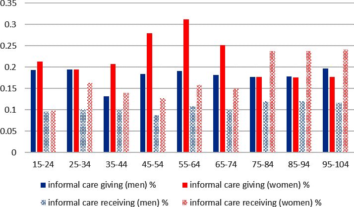
Need and provision of informal care (in percentages in 2025). Source: Own simulations.
3.4. Labour market participation and labour supply
The modelling of labour market participation is a key element in MIDAS_CH, as interruptions and reductions in employment significantly determine pension income after retirement. Since the goal of our model is to simulate the GPG, the employment- and part-time work rate, especially of women is of particular importance. As in most European countries, the majority of men in Switzerland work full time. However, for women, the picture is a bit more complex. In the EU28, the employment rate of women on averaged 64.1% in 2019. In Switzerland in the same year, 76.3% of women were employed, making it the second highest employment rate for women compared to the European countries – only surpassed by Iceland (81.9%; FSO, 2020b). However, the labour market participation of mothers is much lower than that of childless women (Ravazzini, 2018). Switzerland also ranks second in terms of part-time employment among women. In 2019, 62.7% of employed women in Switzerland worked part-time according to the European definition18 (2010: 60.8%) – a percentage only surpassed by the Netherlands (FSO, 2020b).
The conclusion is that although the overall employment rate of women in Switzerland is high, it is often at a reduced employment level. To fully capture the heterogeneity of work intensity, we model it in three steps. First, whether a man or woman works or not is modelled by combining the aforementioned alignment information (see Table 1) with the results of a logistic regression model, with arguments age, civil state and previous work status (employed, unemployed, other inactive). Next, given that a person works, we use the results of a logistic regression model (referring to gender, number of children below age 11 and age 15, civil status, age, and education level) and the alignment information to simulate whether the person works part-time or full-time. The third and final step then models the extent of part-time work for those that are selected to work part-time in the first step. Here we distinguish three groups i) less than 50% of full time, ii) between 50% and 69% of full-time, and, iii) between 70% and 89% of full time. These three groups match with the dimensions of the projections from the FSO (FSO, 2020c) that we use in our alignment tables.
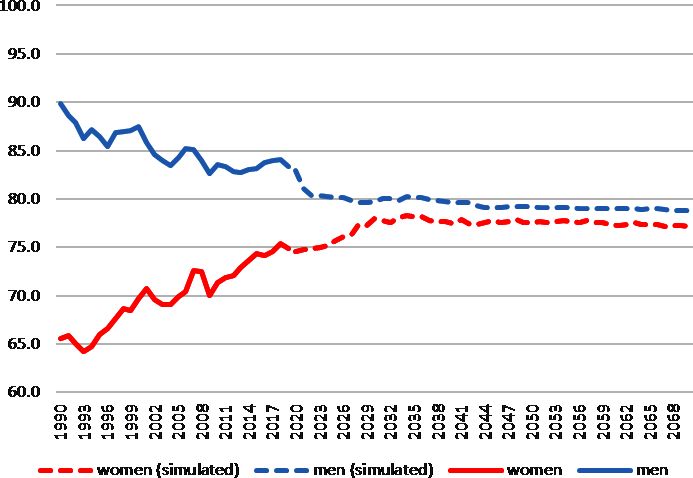
With regard to labour market participation at the extensive and intensive margins, we extended the projections of the FSO from 2050-2070. Figure 4 illustrates the actual and projected labour market participation of men and women in Switzerland. The activity rate of men is declining mainly because of demographic ageing, and partially due to increasing educational attainment levels that delay labour market entry. These developments are also at play with women, but their impacts are more than compensated by the strong increase in the activity rates of women, especially in the middle aged groups, which is driven by a rising level of education and other factors, such as measures to better reconcile work and family life, interest in careers and the need to contribute to household income (FSO, 2020c). It is assumed that the labour market participation of men and women will further converge and stabilise (see Dekkers et al., 2022, for a further discussion).

Actual and projected labour market participation of men and women aged between 15 and 64.. Source: FSO (2021c), own simulations.
In 2019, around 18% of men worked part-time, compared with 60% of women. For this reason, women have significantly lower FTE employment rates than men, especially those of family age. Assuming a better reconciliation of family and work, the FTE employment rate of women will increase significantly by 2050 and a trend towards more part-time employment among men is expected. However, the FTE employment rate of women will still be significantly lower than that of men (FSO, 2020c).
3.5 Early and late retirement
In the years between 2018 and 2020, the early retirement rate one year before the regular (statutory) retirement age was 39% for men (at age 64) and 30.4% for women (at age 63). These rates are declining compared to the 2006-2009 period (when it was 47.1% for men and 43.2% for women) (FSO, 2022b). As early retirement is affected by health status, the probability of early retirement is estimated according on age and educational attainment level, an interaction variable of age and education and whether a person received informal help from relatives, acquaintances or neighbours for health reasons. To ensure consistency with forecasted rates of early retirement, the extent of early retirement is aligned by gender, age and year of simulation.
3.6 Immigration and emigration
Switzerland is a migration country, and the MIDAS_CH model therefore has to allow for immigration and emigration. Each year, around 145.000 people immigrate, while around 126.000 people emigrate. The population is around 8 million. In 2019, Switzerland had approximately 17 immigrations and 15 emigrations per 1000 inhabitants, a rate higher than that of other Western European countries of similar sizes, such as Austria (12 / 8 per 1.000), Belgium (13 / 9 per 1.000), and the Netherlands (12 / 6 per 1.000).19 In 2018, the share of immigrant population in Switzerland equals 29.7%. Apart from micro-states, such as Andorra and Liechtenstein, this is one of the highest percentages in Europe, only surpassed by Luxembourg.
Moreover, the profile of immigrants in Switzerland is somewhat different than in EU countries. According to the Swiss Mobility Migration Survey, immigration to Switzerland is mainly motivated by professional reasons (Steiner and Wanner, 2019). 73% of the immigrants benefited from the “Agreement on the Free Movement of Persons" (AFMP)20 with the EU. The contribution of other types of migrants (1.7% labour migrants from outside the EU, 17% accompanying family members; and 5.5% humanitarian migrants (OECD, 2020) is limited.
According to the projections of the Swiss FSO (FSO, 2020c) both immigration and emigration will increase further in the coming years. As people born during the baby boom in the 1960s gradually reach retirement age, Swiss companies will rely increasingly on foreign labour to fill the gaps (Beerli et al., 2021). Due to the greater mobility of people with a high level of education, who will make up the majority of migrants in the coming years, not only the number of immigrants but also the number of emigrants will increase. In the long term, however, migration would decrease as the European population ages and several countries will experience population decline (FSO, 2020c).
This high proportion of migrants, and the projected developments of immigration and emigration make it necessary for MIDAS_CH to include migration. Furthermore, we decided to model emigration and immigration separately as the age and gender distribution of immigrants and emigrants differs greatly. Finally, we aimed to align our modelling based on the projections of the Swiss FSO (2020c).21
3.6.1. Modelling of immigration
With regard to the modelling of immigration, two challenges arise. First, the characteristics of new immigrants are by definition unknown. This includes the panel history and weighting information needed for the shared weights approach (Schonlau et al., 2013). This can be resolved by the donor approach (Duleep and Dowhan, 2008) by which existing individuals in the dataset are selected to represent prospective immigrants. This donor sample is then cloned and added to the existing dataset. An additional problem is that immigrants often enter the country as households while the alignment tables are expressed in numbers of individuals. We therefore follow Chènard (2000). See Dekkers (2015), O’Donoghue et al. (2010) for a discussion on modelling this in LIAM2.
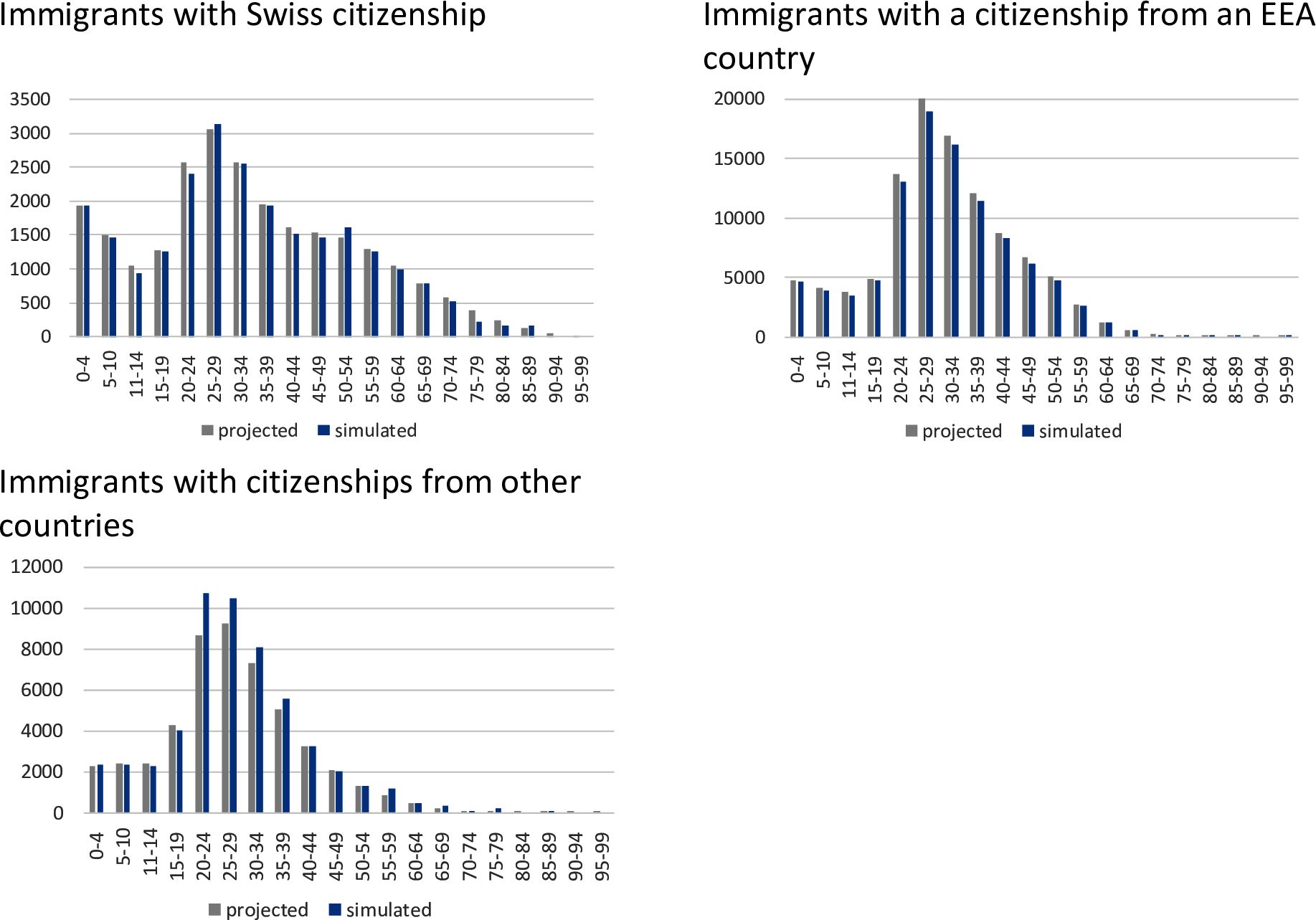
Since the sociodemographic characteristics of immigrant differ by country of origin (FSO, 2019), we have grouped all individuals in the model into three areas, based on country of birth: Switzerland (returning emigrants), the European Economic Area, and other countries. The alignment procedure is based on the projections of the FSO (FSO, 2020c, Scenario A-00-2020), which are made for these three groups. Figure 5 illustrates the age distribution of immigrants by the three regions of origin. Figure 5 compares the projections (FSO, 2020c) and the results of the simulation.

Age distribution of immigrants, by citizenship (2025). Source: Projections by FSO (2020c), base scenario A-00-2020, own simulations.
3.6.2. Modelling of emigration
Modelling of emigration is broadly analogous to the modelling of immigration. However, in the case of emigration, households are not cloned but removed from the dataset. Nevertheless, the households that emigrate must be selected, and the total number of emigrating persons must correspond to the projections of the Swiss Statistical office (FSO, 2020c). To identify the households with the highest probability of emigration, we use the results from Wanner (2021), model 3) to simulate the individual probabilities of emigration. In a second step, we compute the estimated average probability of emigration at household level. Finally, we use the Pageant algorithm again to select households for emigration, and these are removed. Because individuals with different citizenships may live together in one household, households were categorized according to the most common citizenship within the household.22 The alignment is performed, as in the case of immigration, according to projections of the Swiss Statistical office (FSO, 2020c, Scenario A-00-2020), by gender and age. Analogous to our modelling of immigration, we divided the alignment matrix into three areas (Switzerland, European Economic Area, and other countries), as proposed in the MOSPI Report (2020).
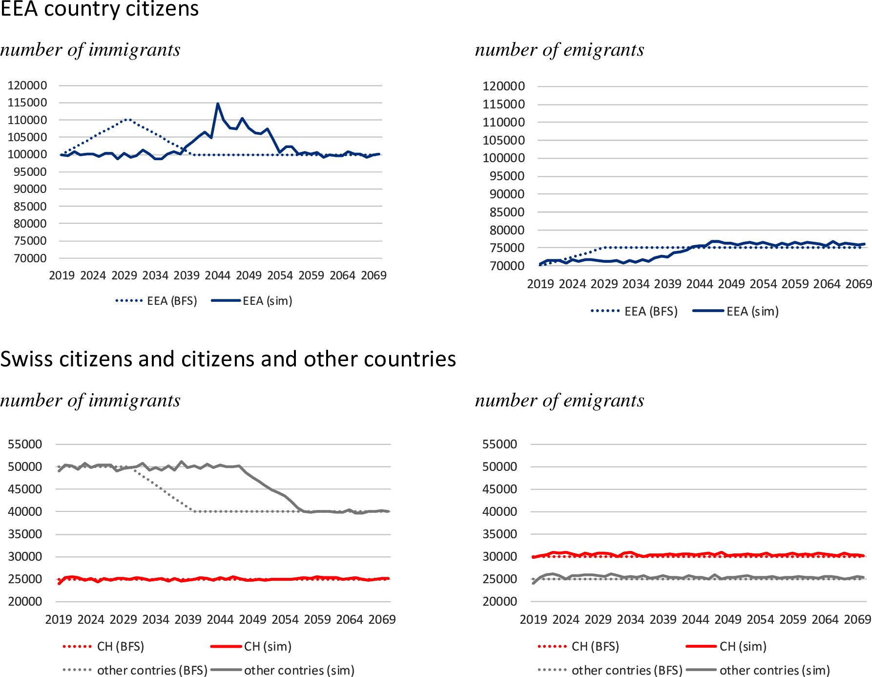
Figure 6 shows the projected (FSO, 2020c) and the simulated number of immigrants and emigrants. The graphs show that the steadier the predicted figures are, the more accurate the results of the alignment process. This is because any deviations from the selection process are carried over to the next period.

Projected and simulated numbers of migrants by citizenship (2019-2070). Source: Projections by Swiss FSO (2020c). base scenario A-00-2020, own simulations.
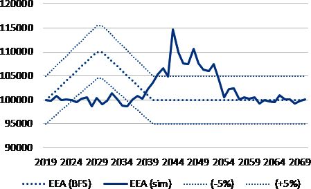
The deviation of the simulations from the projection remains however for most of the simulated years within a range of (+/- 5% points), as shown in Figure 7, which depicts the projected number of immigrants (dashed line, +/- 5% confidence interval) and the simulated number of immigrants (solid line).

Projected and simulated number of immigrants with EEA citizenship (2019-2070). Source: Projections by Swiss FSO (2020c). base scenario A-00-2020, own simulations.
4. Simulation of pension income
The Swiss pension system consists of three pillars. The 1st pillar, which consists of the old-age and survivors' insurance (OASI), the disability insurance (DI) and means-tested supplementary benefits (SB), is a publicly financed pay-as-you-go system. The 2nd pillar is an employer-based, fully funded occupational pension system while the 3rd pillar is a voluntary, individual, tax-privileged private provision in addition to the first and second pillars (see Kirn and Baumann, 2021).
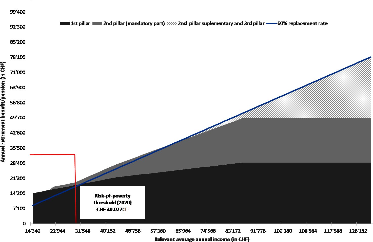
Figure 8 illustrates the relationship between annual retirement benefit and the average annual lifetime income, assuming an uninterrupted working career of 44 years and applying a conversion rate equal to 6.8% for the mandatory part of the 2nd pillar pension income. The 1st pillar, represented as a dark grey area, aims at providing a basic retirement income. The mandatory part of the 2nd pillar (light grey area) and the supplementary part of the 2nd pillar and 3rd pillar (hatched area) should enable the “continuation of the accustomed way of life”. The three pillars are coordinated in such a way that a replacement rate equal to 60% of the average annual lifetime income is achieved (blue line). By contrast, for wages below CHF 30,072, which is the risk-of-poverty threshold,23 the benefit target of 60% is already met by the 1st pillar pension alone. However, the maximum pension benefit one can receive from the 1st pillar alone (which is CHF 28,680) is itself below the at-risk-of-poverty threshold. In 2019, 16% of the elderly population received a pension income (excluding notional rent) below the risk-of-poverty threshold, which is slightly below the European average24 (FSO, 2021a).

Amount of annual retirement pension per given average annual income. Source: Own computations.
Next we discuss the simulation of 1st and 2nd pillar pension income in more detail. The model does not cover the 3rd pillar, so we will not discuss this further.
4.1 Simulation of 1st pillar pension income
The 1st pillar includes old age, survivors and disability benefits (OASI/AHV & DI/IV) as well as supplementary benefits (SB/EL). In old age or in case of death and injury, the OASI/DI takes over the insured person’s livelihood. If the income from pensions is not sufficient to ensure subsistence, means-tested supplementary benefits (SB) cover the necessary living requirements. OASI insurance is compulsory for all residents of Switzerland, including non-working persons, students, people receiving public transfers (such as unemployed and disabled workers), and the self-employed. The system is financed by a proportional contribution on earned income, without a cap.
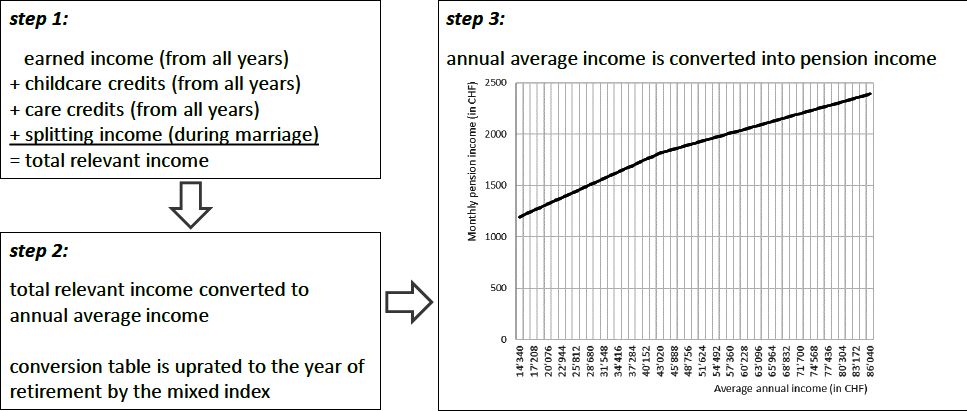
The OASI pension income depends on the number of eligible contribution years and the ‘relevant’ annual income, which is the sum of revalued incomes (employment incomes, non-employment contributions, split income25 are uprated according to the mixed index)26 and the sum childcare and care credits. Childcare and care credits are warranted to those persons who care for children under 16 years of age27 or relatives in need of care during their contribution years.28 Both credits correspond to three times the minimum annual pension (CHF 3,585 per month, which is about 60% of the median income of women (CHF 6,067 per month) (FSO, 2020b).
Figure 9 illustrates the conversion of earned, split income and credits to ‘relevant’ pension income, which is then used as the basis of the 1st pillar pension benefit. The conversion of the annual average income to pension income is based on a pension formula, which is linked to a parameter table and indexed by the mixed index.

Conversion of earned income and credits to pension income. Source: Own illustration.
A full pension is paid to anyone who has paid AHV contributions without interruption every year from the age of 20 up to the statutory retirement age (SRA);29 missing contributions years therefore result in partial pensions. However, since the entire population is compulsorily insured, incomplete contribution careers are rare, except for those immigrants that have not been in Switzerland for their entire working life.
Figure 9 shows that the transfer from annual average income to pension income is highly degressive. Through the use of redistributive parameters such as care credits and income splitting, the benefits depend weakly on income and in a linear way on the number of contribution years.
Besides being highly degressive, the 1st pillar pension income is subject to both a minimum and a maximum benefit. But here too the Beveridgean character of the pillar reveals itself: the former (CHF 14,340 or €14,704 per year) is half of the latter (CHF 28,680 per year), while the maximum benefit remains below the risk-of-poverty threshold (CHF 30,072 per year) (see Figure 8). Finally, the pension of a married couple is capped at 150% of the maximum individual pension. If a married couple decides to divorce, all income earned during the spouses' marriage is divided equally between both parties. In case of death of a beneficiary, the surviving partner gets a benefit equal to at most 80 percent of the deceased spouse’s 1st pillar pension. If someone can claim a 1st pillar or disability pension at the same time as the widow’s or widower’s pension, only the higher pension will be paid.
4.2 Simulation of 2nd pillar pension income
The 2nd pillar of the Swiss pension system is the occupational pension,30 which became compulsory for all employees of 17 and older in 1985. It consists of a mandatory base part and a voluntary supplementary part. To ensure a steady replacement rate (see Figure 8), the minimum and maximum contribution thresholds of the mandatory part are linked to the pension level of the first pillar, whereas the minimum (maximum) threshold is 1.5 (three) times the maximum OASI annual pension. The supplementary - voluntary part - covers income above the maximum eligible annual salary. Due to the lower contribution ceiling of the mandatory part, low-income individuals (mostly female workers) are often not covered by the second pillar, resulting in a low coverage rate of the second pillar (49% in 2019) compared to the almost full coverage of the 1st pillar pension system (Kuhn, 2020).
The mandatory part of the 2nd pension pillar is subject to strict regulation with regard to minimum contribution rates and minimum interest rates on accumulated assets. Furthermore, the nominal annuity B is a function of the accumulated retirement capital K and a minimum conversion rate , as .31 Since the conversion rate depends on life expectancy and the interest rate, a lower conversion rate can be expected in the future if life expectancy increases and interest rates are low (see projection in section 2.1). However, since a reduction in the conversion rate has a significant impact on pension income, two different scenarios are simulated by assuming a reduction in the conversion rate from the current 6.8% to 5.2% and a constant conversion rate. The supplementary and voluntary part of the 2nd pension pillar, is not subject to such strict regulations, and pension funds are therefore free to set contribution rates, the interest rate and the conversion rate. They can also apply lower income thresholds for part-time workers. Unfortunately, there are no official statistics on average contribution rates, interest rates or conversion rates of the supplementary part of the 2nd pillar. Therefore, in the simulation, only the mandatory part is simulated. Although the majority of insured individuals legally fall under defined contribution (DC) plans, the strict regulation of the mandatory part and income guarantees make that system resemble more defined benefit (DB) plans in practice.
As in the case of divorce, each spouse is entitled to half of the credit balance accumulated jointly during the marriage. We simulate the pensions of married and divorced couples accordingly. Furthermore, in case of death, the surviving spouse is entitled to a survivor’s pension equal to 60% of the retirement pension or 100% of the disability pension of the deceased spouse, which is also simulated.
5. Main simulation results
As an application of the new MIDAS_CH model, we simulate the income trajectory of individuals over their entire lifespan and the resulting pension income and analyse the Gender Pension Gap (GPG). The gender pension gap is usually much higher than the gender pay gap, since the income differences between the sexes and gendered behaviour (prevalence of part-time work and leaves due to care obligations) add up. As however the redistributive elements within pension systems are designed to compensate for losses in earnings due to non-standard working careers and/or non-standard family arrangements (Möhring, 2021), the relationship between the earnings gap and differences in labour market participation on the GPG is not linear (Kirn and Dekkers, 2022).
According to the Eurostat definition of the GPG, pension income includes gross retirement pensions, gross survival pensions as well as the means-tested supplementary benefits for the elderly. People with zero pensions, as well as those below age 65 are excluded from the calculation. In addition to this general definition of the GPG, there are numerous variants that can be distinguished based on Dekkers’ four dimensions (Dekkers et al., 2022). First, the underlying definition of pension income can be restricted on retirement pensions (covering all pillars), both old-age and survivors’ pensions, and exclude the means-tested “guaranteed minimum income” (denoted SB) for the elderly. As we focus on pension income, we report the GPG based solely on retirement income, excluding SB.
Second, the standard definition of the GPG excludes the 65+ without a pension and is based on the assumption that people who do not have a retirement benefit are not retired. However, it may in some cases be relevant to construct a variation of the GPG that extends the standard definition of the GPG by including zero pensions. The latter GPG can then be interpreted as a combination of the standard GPG and the gender pension coverage gap, which measures the extent to which women have their own independent access to pension system benefits (European Commission, 2018). It is of course not very relevant for the pension benefit of the 1st pillar only, where the coverage gap is close to zero because persons who are not gainfully employed must also contribute to the OASI. But this is in contrast to the 2nd pillar, where the overall coverage rate is 49% in 2019 (Kuhn, 2020), and we therefore can expect important gender differences. Hence, comparing the standard GPG with that including zero-values is still very relevant for the pension income from both pillars together. In doing so, we include zero 2nd pillar pensions in our analysis to compute the GPG.
Third, the standard GPG compares the mean gross benefits of men and women. However, the GPG can also be calculated by using other measures of location, such as percentiles or quartiles. In this article, we will present the GPG at the mean, the 25th and 75th percentile. Furthermore, we measure pension inequality by the P75/P25 ratio. To analyse the development of the GPG, we compare the simulated P75/P25 ratios to the 2019 statistics.
Fourth, the GPG can be derived separately for age groups. As in other studies (Bonnet et al. (2006); Halvorsen and Pedersen (2019)), we focus on one birth-cohort of individuals born in 2000. This cohort will reach the statutory retirement age of 65 in 2065. The dynamic simulation covers the entire span of the contribution obligation, i.e. 44 years for the 1st pillar and 40 years for the 2nd pillar. At the simulation horizon in 2070, we simulate pensions of those that retire at the SRA as well as early retirement (two years before SRA) and retirement five years later, since retirement at a later point in time is also possible. In the standard measure of the GPG we compute the GPG at the SRA.
Although the selected simulation horizon for the 2000 birth cohort covers the entire contribution period, it does not automatically follow that the life histories analysed have no contribution gaps. As explained earlier, migration at an age older than 21 leads to gaps in contributions, even in the 1st pillar of the Swiss pension system. For this reason, we analyse the pension income of immigrants separately.
In the next section, we analyse the current GPG at SRA. To analyse the impact of the most recent pension reform – the increase in the SRA of women from 64 to 65 – we simulate the pension incomes and compare the GPGs in 2070 (policy scenario I and II). Next, we simulate a reduction of the conversion rate of the mandatory part of the 2nd pillar – which is a likely future policy scenario – and analyse its potential impact on the GPG in 2070 (policy scenario III).
5.1 The current situation – GPG in 2020
The current GPG is determined on the basis of the new pension statistics (Neurentenstatistik, NRS), as it is a full survey that describes how many people have recently received a retirement pension or make a lump-sum withdrawal from the 2nd (and 3rd) pillar pension system (FSO, 2022b).
Table 2 reports the percentiles of observed 1st pillar pension income of people receiving their first retirement pension at their SRA, which is 64 years for women and 65 for men (FSO, 2022b). Despite the strong redistributive elements of the 1st pillar, women receive a lower 1st pillar pension income across the entire income distribution than men. This is driven by the gendered labour market participation as well as income differences between the sexes.
1st pillar pension income at SRA (in 2020)
| total (65) | women (64) | men (65) | GPG | |
|---|---|---|---|---|
| mean | 23,285 | 21,090 | 23,357 | 9.7% |
| p25 | 21,240 | 19,764 | 21,240 | 6.9% |
| p50 | 23,892 | 21,240 | 23,892 | 11.1% |
| p75 | 27,984 | 23,892 | 27,984 | 14.6% |
| p75/p25 | 1.32 | 1.21 | 1.32 |
-
Source: New pension statistics: individuals at regular retirement age who received their first pension in 2020 FSO (2022b).
With regard to the gender specific quartiles, we find that the GPG is lower at the bottom 25% of the income distribution than at the top 25%. This result may be driven by the regressive character of care credits, which dampen the GPG at the bottom of the income distribution. This is also reflected in the ratio between the pension income and the minimum pension income. The pension income of women in the first quartile is 39% above the minimum pension income, which was CHF 14,220 per year in 2020. The comparable pension income of men is 49% above the minimum pension income. The pension income of men in the top 25% is close to the maximum 1st pillar pension income, which is CHF 28,440 in 2020. For women, on the other hand, the top 25% achieve only about 84% of the maximum pension. This illustrates that the redistributive elements of the 1st pillar have a stronger impact on lower pensions, since the lowest 25% receive more than the minimum pension, but the maximum pension is reached only by the top 25% among men, but not among women. Consequently, pension inequality, as measured by the P75/P25 ratio, is also higher for men than for women.
Table 3 reports the percentiles of observed 2nd pillar pension income (mandatory and supplementary) of new beneficiaries who receive a retirement pension at their SRA (FSO, 2022b). In contrast to the 1st pillar, where 85% of all new pensioners drew their retirement pension upon reaching the SRA, the first withdrawal of a pension from the 2nd pillar would be less focussed around the SRA.31 Here, 36% of all new beneficiaries would draw a retirement benefit before the SRA.32 Furthermore, when interpreting the table, it should be noted that in 2019 43% of male and 52% of female new pensioners opted for the pension in the form of an annuity. Around one-third opted for a lump-sum withdrawal at or before retirement age (33% among men and 34% among women). About 24% of men and 14% of women new recipients opted for a combination of the two. There are also significant differences between the sexes in terms of lump-sum withdrawals. Lump-sum withdrawals from the second pillar are much higher for men than for women (CHF 160,000 vs CHF 49,800 in 2020),33 which leads to a comparatively lower pension income for men. Thus, statements about the GPG based on this database are of limited value, which also applies to the sum of 1st and 2nd pillar pension income (see Table 4).
2nd pillar pension income at SRA (in 2020)
| total (65) | women (64) | men (65) | GPG | |
|---|---|---|---|---|
| mean | 25,353 | 15,571 | 25,884 | 39.8% |
| p25 | 12,267 | 6,408 | 12,836 | 50.1% |
| p50 | 20,897 | 12,000 | 21,385 | 43.9% |
| p75 | 32,084 | 20,681 | 32,525 | 36.4% |
| p75/p25 | 2.62 | 3.23 | 2.53 |
-
Source: New pension statistics: individuals at regular retirement age who received their first pension in 2020 FSO (2022b).
1st and 2nd pillar pension income at SRA (in 2020)
| total (65) | women (64) | men (65) | GPG | |
|---|---|---|---|---|
| mean | 49,973 | 38,225 | 50,021 | 23.6% |
| p25 | 36,564 | 28,228 | 36,629 | 22.9% |
| p50 | 46,203 | 34,998 | 46,236 | 24.3% |
| p75 | 58,440 | 44,836 | 58,428 | 23.3% |
| p75/p25 | 1.60 | 1.59 | 1.60 |
-
Source: New pension statistics: individuals at regular retirement age who received their first pension in 2020 FSO (2022b).
Compared to the 1st pillar (see Table 2), the gender differences are significantly larger, because the 2nd pillar is considerably less redistributive as it has the character of a DC/DB hybrid. At the median income, the GPG of the occupational pension amounts to 43.9%. This is because women are more likely than men to forego or reduce their gainful employment when they become mothers (Budig and England, 2001; England et al., 2016; Ehrlich et al., 2020; Gash, 2009; Gutiérrez-Domènech, 2005), take up informal care tasks (Ciccarelli and Van Soest, 2018; Earle and Heymann, 2012; European Commission, 2021a; Evandrou and Glaser, 2003; Heitmueller, 2007; Henz, 2004; Kuhn and Ravazzini, 2017), which may affect their earnings for this and other reasons (Busch, 2020; Eurofound, 2020; Möhring, 2021; Sefton et al., 2011). As a consequence, with regard to pensions, women are more likely than men to earn wages that are below the entry threshold for occupational pension provision (Kuhn, 2020).
Note that pension inequality is higher in this case for women than for men. The reason lies in the higher career variation among women (Möhring, 2021) than among men, even if both meet the earnings requirement for the 2nd pension pillar. Pension inequality is reflected in the P75/P25 ratio, which is much higher than in the 1st pillar pension income statistics (see Table 2), for both men and women.
Since both pillars contribute about the same amount to pension income on average, gender differences are also reflected in total pension income (see Table 4). However, since for the 1st pillar the GPG is lower for the lower income percentiles while for the 2nd pillar it is the other way around, for total pension income the GPG across the entire income distribution is around 23%.
5.2 Policy scenario I: SRA of women remains at 64 – GPG in 2070
The AHV 21 reform, which among other things provides for an increase in the retirement age for women from 64 to 65, was adopted in September 2022. To analyse the impact of an increase in retirement age, we compare the simulated 1st pillar pension with a retirement age of 64 for women (scenario I) to the pension income with a retirement age of 65 for women (scenario II).
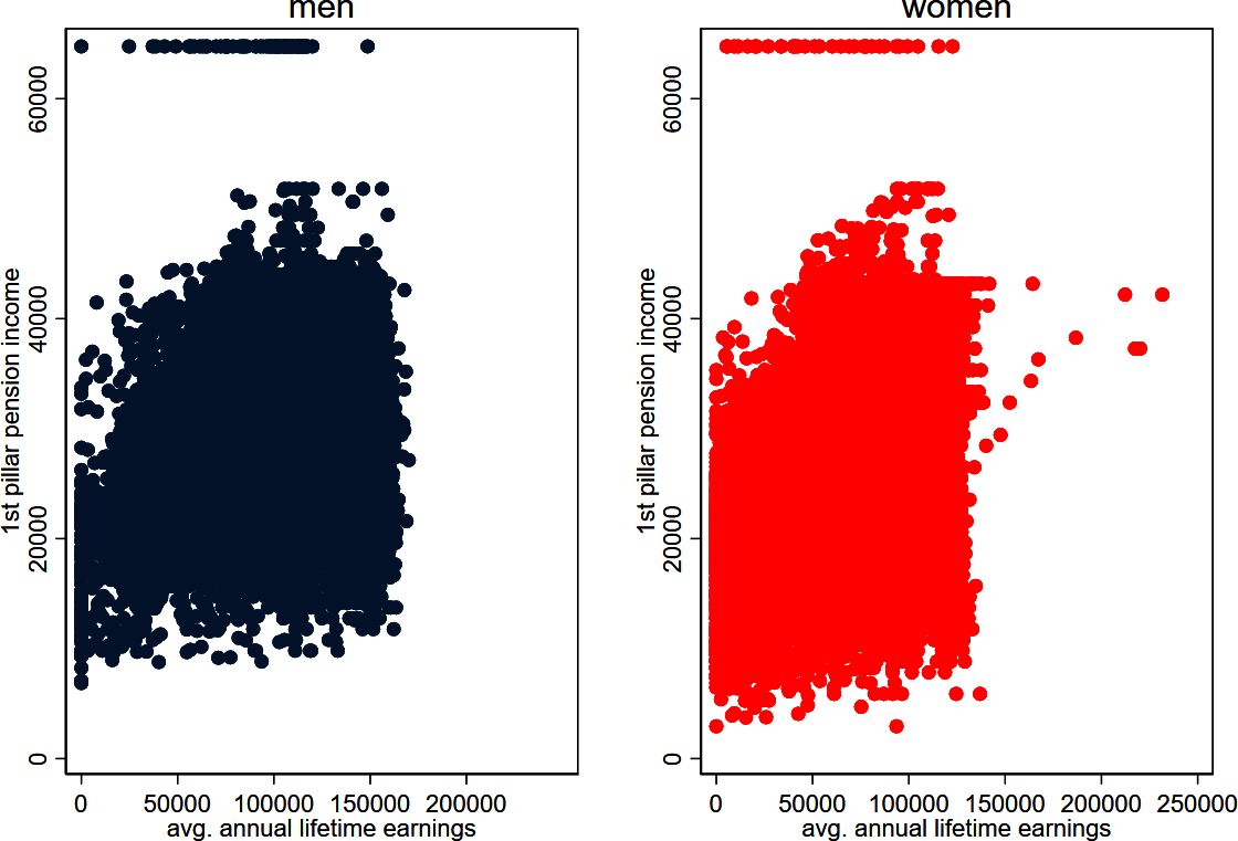
The simulated 1st pillar pension incomes in year 2070 are illustrated by the scatterplot (Figure 10), whereas it is assumed that the SRA is at the age of 65 for both men and women.34 There is a positive correlation between average lifetime income (x-axis) and 1st pillar pension income (y-axis), but the variance is greater for women, which is due to the redistributive elements that predominantly benefit women. In addition, the upper limit of the pension income of the 1st pillar (which is twice the minimum pension income) is expected to be 43,174 CHF in 2070, as well as the maximum pension income of married couples, which is expected to be 64,761 CHF.

Simulated 1st pillar pension income (all retirees, in 2070). Source: Simulated data, based on SILC 2018. SRA for women: 64, SRA for men: 65 years.
Table 5 reports the percentiles of the simulated 1st pillar pension income at SRA in the year 2070. According to the projections, women would continue to receive a lower pension income from the 1st pillar than men across the entire income distribution in 2070. However, compared to 2019, the gender gap would narrow significantly in 2070 and become marginal at the top 50% income distribution. This effect is mainly due an increase in the number of women reaching a maximum pension. The 1st pillar pension income at the 25th percentile of women is 43% above the minimum pension income, for men it is 66%, which indicates that the relative income distribution at the bottom 25% of the income distribution will not change significantly.35 However, with regard to the top 75% of income distribution, we expect that the 1st pillar pension income at the 75th percentile of women (men) is 94% (98%) of the maximum pension income, which means that almost all men and women in the top quartile would receive the maximum 1st pillar pension income, which would however, be below the risk-of-poverty threshold. Compared to 2019, we expect women in the top 75% of income distribution to catch up and the GPG in the top income distribution to become smaller.
Simulated 1st pillar pension income at SRA (2070) – simulation variant with SRA of women of 64
| mean | p25 | p50 | p75 | p75/p25 | |
|---|---|---|---|---|---|
| total population | 37,391 | 33,614 | 38,722 | 42,044 | 1.25 |
| women | 35,682 | 30,781 | 37,283 | 40,672 | 1.32 |
| men | 39,027 | 35,806 | 40,070 | 42,376 | 1.18 |
| GPG | 8.6% | 14.0% | 7.0% | 4.0% | |
| non-immigrants | 37,297 | 33,463 | 38,680 | 41,905 | 1.25 |
| women | 35,642 | 30,711 | 37,179 | 40,642 | 1.32 |
| men | 39,131 | 36,098 | 40,304 | 42,470 | 1.18 |
| GPG | 8.9% | 14.9% | 7.8% | 4.3% | |
| immigrants | 38,138 | 34,821 | 39,055 | 42,193 | 1.21 |
| women | 36,526 | . | . | . | . |
| men | 38,534 | 35,057 | 39,276 | 42,193 | 1.20 |
| GPG | 5.2% | . | . | . |
-
Source: own computations. SRA for men 65 years and women 64 years. Quantile incomes of female immigrants are not reported due to the relatively small number of cases in the simulated dataset.
This is also reflected in pension inequality, where the P75/P25 ratio of women (men) increased from 1.02 (1.03). to nearly 1.32 (1.18). Hence we see a greater inequality of 1st pillar pension income. This effect may be explained by a higher share of women having tertiary educational attrition, which is associated with higher wages, leading to a reduction of the GPG in the upper income range. However, since labour market participation as well as the extent of part-time employment are positively correlated with the level of education, this leads to a larger variance in women’s lifetime earnings. This finding is in line with Kuhn and Ravazzini (2017) who observe that women in couples are more likely to work if they earn higher wages, however, working women with higher wages tend to work slightly less than working women with lower wages.
The simulation results suggest that pension income of male immigrants would still be slightly below the pension income of male non-immigrants across the entire income distribution. However, the pension income of female immigrants would be at the mean slightly above the pension income of female non-immigrants. This result may be driven by the on average higher labour market participation of female immigrants in comparison with female non-immigrants.
5.3 Policy scenario II: SRA of women increases up to 65 – GPG in 2070
In policy scenario II we analyse the impact of an increase in the SRA of women from 64 to 65, which was adopted in September 2022. The simulation results suggest, that the 1st pillar pension income of women increases slightly across the income distribution – except in the top 75% of the income distribution (see Table 6). This effect may be driven by the circumstance, that women may achieve a higher average lifetime income due to the prolongation of working life. However, these effects are marginal.
Simulated 1st pillar pension income at SRA (2070) – simulation variant with SRA of women of 65
| mean | p25 | p50 | p75 | p75/p25 | |
|---|---|---|---|---|---|
| total population | 37,500 | 33,963 | 38,754 | 42,193 | 1.24 |
| women | 35,752 | 31,281 | 37,540 | 40,604 | 1.30 |
| men | 39,154 | 35,751 | 40,800 | 42,780 | 1.20 |
| GPG | 8.7% | 12.5% | 8.0% | 5.1% | |
| non-immigrants | 37,377 | 33,652 | 38,734 | 42,143 | 1.25 |
| women | 35,704 | 31,248 | 37,517 | 40,612 | 1.30 |
| men | 39,212 | 35,879 | 41,049 | 42,781 | 1.19 |
| GPG | 8.9% | 12.9% | 8.6% | 5.1% | |
| immigrants | 38,422 | 35,255 | 39,045 | 42,193 | 1.20 |
| women | 36,649 | . | . | . | . |
| men | 38,888 | 35,311 | 39,621 | 42,760 | 1.21 |
| GPG | 5.8% | . | . | . |
Table 7 reports the percentiles of the simulated 2nd pillar pension income at SRA in year 2070 with a conversion rate of 6.8% on mandatory pension savings. According to the projections, the GPG would decline across the entire income distribution compared to 2020 (see Table 3). However, when interpreting these ratios it must be kept in mind that Table 7 reports the mandatory part of the 2nd pillar pension income, which is capped by the statutory maximum qualifying annual salary. Furthermore, because lump-sum withdrawals have not been simulated, the 2nd pillar pension income is comparatively higher.
Simulated 2nd pillar pension income at SRA (2070) – simulation variant with SRA of women of 65 and a constant conversion rate of 6.8%
| mean | p25 | p50 | p75 | p75/p25 | |
|---|---|---|---|---|---|
| total population | 30,315 | 20,112 | 29,624 | 41,393 | 2.06 |
| women | 23,636 | 14,484 | 24,329 | 32,084 | 2.22 |
| Men | 36,636 | 27,052 | 39,030 | 45,180 | 1.67 |
| GPG | 35.5% | 46.5% | 37.7% | 29.0% | |
| non-immigrants | 29,961 | 19,808 | 29,183 | 40,985 | 2.07 |
| women | 23,684 | 14,482 | 24,457 | 32,079 | 2.22 |
| Men | 36,851 | 27,229 | 39,142 | 45,287 | 1.66 |
| GPG | 35.7% | 46.8% | 37.5% | 29.2% | |
| immigrants | 32,972 | 21,690 | 35,132 | 42,679 | 1.97 |
| women | 22,731 | . | . | . | . |
| Men | 35,662 | 24,683 | 38,469 | 43,400 | 1.76 |
| GPG | 36.3% | . | . | . |
-
Source: own computations. SRA for men and women: 65 years. Second pillar: Mandatory pension, conversion rate: 6.8%. Quantile incomes of female immigrants are not reported due to the relatively small number of cases in the simulated dataset.
The change in the GPG across the income range is interesting however. The simulation results suggest, that women at the 25th percentile receive 46.5% of the pension benefit of men, which is only a slight decrease of the GPG down from 50.1 (see Table 3). However, as 2nd pillar pension entitlements are strongly related to lifetime income, this differences reflecting men’s higher lifetime income. This effect is aggravated as women, who work part-time and have low salaries are more strongly affected by the income threshold (coordination deduction) for contributive income. However, in 2070 the coverage rate of the 2nd pillar of women is almost 100%, compared to around 49% in 2020. Thus, almost all female pensioners in 2070 receive a simulated pension from the 2nd pillar, although in the first quartile the pension income of women is significantly lower than that of men. In the third quartile, however, we observe a catching up process of women. Here the GPG of the 2nd pillar pension income at the 75th percentile will decline from 36.4% in 2020 to 29% in 2070. Overall, it can be said that women are catching up, especially in the upper income brackets. This is because the intensity of work increases with higher formal education, which in turn leads to comparatively higher lifetime earnings for women.
For the 2nd pillar, the pension income of retirees with an immigration background is also larger than that of retirees without an immigration background. This effect may be driven by the fact that some of the immigrants are very well educated and can thus earn a correspondingly high lifetime income, but the higher labour market participation of immigrants is also a factor. This finding is in line with Steiner and Wanner (2019), who observe during the past decade an increased proportion of highly skilled migrants, which is driven by a shortage of human resources in some high value-added sectors, such as health, IT services and specific financial sectors.
The 75/25 ratio, which reflects pension income inequality, has decreased. However, the results in Table 7 confirm those in Table 3 in that inequality as measured by the proportional difference between the 75th and 25th percentile, would remain higher for women than for men.
The simulation results suggest, that the GPG of the simulated overall pension income (see Table 8) will be lower for the higher income deciles. This result is remarkable in that the relative share of pension income from the second pillar in total income increases as income rises. Thus, the share of pension income from the second pillar is 31% at the 25th percentile but 45% in the top 75% of the income distribution. However, since the second pillar has a lower redistributive effect than the first pillar, the decrease in GPG reflects the much higher labour market participation of women at the 75th percentile of income distribution of women.
Simulated 1st and 2nd pillar pension income at SRA (2070) – simulation variant with SRA of women of 65 and a constant conversion rate of 6.8%
| mean | p25 | p50 | p75 | p75/p25 | |
|---|---|---|---|---|---|
| total population | 67,815 | 55,341 | 68,940 | 83,238 | 1.50 |
| women | 59,387 | 47,277 | 61,608 | 71,631 | 1.52 |
| Men | 75,789 | 65,098 | 79,654 | 86,900 | 1.33 |
| GPG | 21.6% | 27.4% | 22.7% | 17.6% | |
| non-immigrants | 67,338 | 54,787 | 68,612 | 82,786 | 1.51 |
| women | 59,388 | 47,126 | 61,813 | 71,576 | 1.52 |
| Men | 76,064 | 65,608 | 80,013 | 87,232 | 1.33 |
| GPG | 21.9% | 28.2% | 22.7% | 17.9% | |
| immigrants | 71,394 | 58,799 | 73,576 | 85,190 | 1.45 |
| women | 59,381 | . | |||
| Men | 74,550 | 62,037 | 77,676 | 85,843 | 1.38 |
| GPG | 20.3% | . | . | . |
-
Source: own computations. SRA for men and women: 65 years. Second pillar: Mandatory pension, conversion rate: 6.8%. Quantile incomes of female immigrants are not reported due to the relatively small number of cases in the simulated dataset.
5.4 Policy scenario III: Reduction of conversion rate – GPG in 2070
Up to now, the simulation results have described the reference scenario, which assumes a constant conversion rate at 6.8%. However, the conversion rate in practice is an ad hoc function of life expectancy among other things, so we can expect that it will decrease over time. Hence, we developed a first alternative scenario where we assume that the conversion rate would gradually decline from 6.8 to 5.2%.
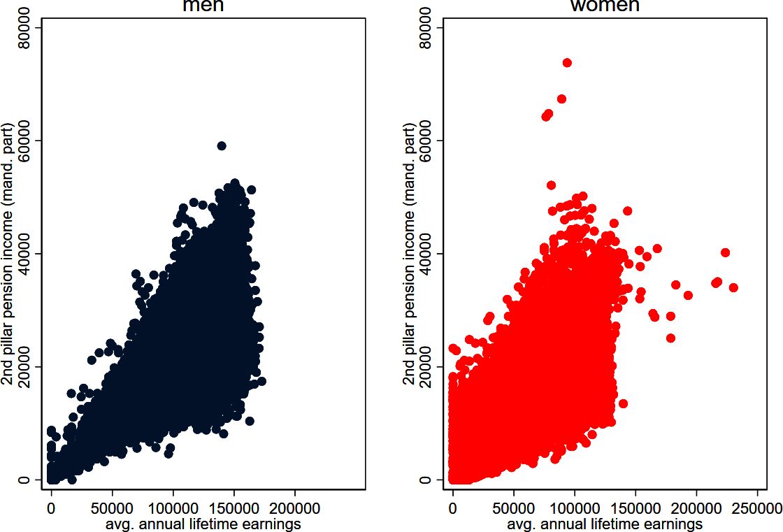
Figure 11 illustrates the simulated the simulated 2nd pillar pension income (mandatory part) at SRA, where a conversion rate of 5.2% is assumed, given the increased life expectancy and low interest rate expectations. When interpreting the results, it should be taken into account, that a reduction of the conversion factor from 6.8% (status quo) to 5.2% (as assumed for 2070) will lead to a reduction of pension income by 23.5% (1-5.2/6.8=0.235).

Simulated 2nd pillar pension income (mandatory part, 5.2%, all retires, in 2070). Source: Simulated data, based on SILC 2018.
Table 9 reports the simulated 2nd pillar pension income (mandatory part) at SRA, where a conversion rate of 5.2% is assumed, given the increased life expectancy and low interest rate expectations. Since the lower conversion rate reduces the pension income of both men and women equally, the GPG does not change. On average, 2nd pillar pension income would decrease by 23.5% if the conversion rate were reduced from 6.8% to 5.2%.
Simulated mandatory part of the 2nd pillar pension income at SRA (in 2070) – simulation variant with decreasing conversion rate.
| mean | p25 | p50 | p75 | p75/p25 | |
|---|---|---|---|---|---|
| total population | 23,196 | 15,380 | 22,653 | 31,654 | 2.06 |
| women | 18,102 | 11,234 | 18,634 | 24,552 | 2.19 |
| men | 28,016 | 20,687 | 29,847 | 34,549 | 1.67 |
| GPG | 35.4% | 45.7% | 37.6% | 28.9% | |
| non-immigrants | 22,926 | 15,217 | 22,316 | 31,342 | 2.06 |
| women | 18,139 | 11,177 | 18,703 | 24,538 | 2.20 |
| men | 28,180 | 20,822 | 29,932 | 34,631 | 1.66 |
| GPG | 35.6% | 46.3% | 37.5% | 29.1% | |
| immigrants | 25,220 | 16,587 | 26,866 | 32,637 | 1.97 |
| women | 17,414 | . | . | . | . |
| men | 27,271 | 18,875 | 29,417 | 33,188 | 1.76 |
| GPG | 36.1% | . | . | . |
-
Source: own computations. SRA for men and women: 65 years. Second pillar: Mandatory pension, conversion rate: 5.2%.
Table 10 reports the percentiles of the simulated 1st and 2nd pillar pension income (mandatory part). According to the simulation results the GPG is expected to decline at the mean from 21.6% to 19.8% if the conversion rate were to be reduced. A reduction in the conversion rate would reduce the GPG more for higher incomes, since the relative share of pension income from the 2nd pillar is larger for higher incomes. Pension inequality, measured by the P75/25 would also decline.
1st and 2nd pillar pension income at SRA (2070)- simulation variant with SRA of 65 and a decreasing conversion rate
| mean | p25 | p50 | p75 | p75/p25 | |
|---|---|---|---|---|---|
| total population | 60,696 | 50,463 | 61,552 | 73,592 | 1.46 |
| women | 53,854 | 44,037 | 55,854 | 64,218 | 1.46 |
| men | 67,169 | 58,774 | 70,312 | 76,465 | 1.30 |
| GPG | 19.8% | 25.1% | 20.6% | 16.0% | |
| non-immigrants | 60,303 | 50,166 | 61,309 | 73,124 | 1.46 |
| women | 53,843 | 43,754 | 55,931 | 64,213 | 1.47 |
| men | 67,393 | 59,131 | 70,643 | 76,683 | 1.30 |
| GPG | 20.1% | 26.0% | 20.8% | 16.3% | |
| immigrants | 63,643 | 53,860 | 65,319 | 74,649 | 1.39 |
| women | 54,063 | . | . | . | . |
| men | 66,159 | 56,152 | 68,558 | 75,304 | 1.34 |
| GPG | 18.3% | . | . | . |
-
Source: own computations. SRA for men and women: 65 years. Second pillar: Mandatory pension, conversion rate: 5.2%.
6. Summary and conclusions
As far as we are aware, MIDAS_CH is the first dynamic cross-sectional microsimulation model for Switzerland. It has been developed to assess the pension adequacy of the 1st and mandatory part of the 2nd pillar pension income of the Swiss Pension system. It simulates the life spans of the cohort born in 2018 and migrating individuals with all its underlying demographic and labour market processes, such as labour supply, marriage and divorce, family formation and resolution as well as the need for informal care.
The microsimulation model runs on LIAM2 and has taken the MIDAS_BE model as a source of inspiration and example. As such, it belongs to a class of older -and further developed- models, such as MOSART, SESIM, DESTINIE, T-DYMM. MIDAS_CH is based on the Swiss SILC dataset and aims to ensure consistency with forecasted target proportions. It has an extensive alignment procedure, as well as a dynamic weighting procedure.
With regard to the 1st pillar pension income at SRA in the year 2070, the simulations suggest that the GPG would decline from 9.7% to 8.7%. At the upper half of the income distribution, the GPG would almost disappear. Furthermore, a higher proportion of women would receive a maximum pension. This trend is also reflected in the GPG of the 1st and the mandatory part of the 2nd pillar pension income at SRA. At mean, the GPG would decline only marginal from 23.6% to 21.6%. However, at the top 25% of the income distribution, the gap would narrow significantly and decline from 23.3% to 17.6%. At the bottom 25% of the income distribution, however, the GPG would increase slightly from 23.6% to 27.5%. The catching-up process of women may be driven by two trends: first, compared to earlier cohorts, the share of women with tertiary educational attainment levels would increase, which means that their average wage would increase. This leads to a reduction of the GPG in the upper income range. However, since labour market participation and part-time employment are positively correlated with the level of education, we expect that the variance in women’s lifetime earnings will also increase. Here our research confirms for Switzerland the trends found in other countries (Bonnet et al., 2006; Dekkers et al., 2022; Halvorsen and Pedersen, 2019).
In contrast to the 1st pillar pension system, which has strong retributive elements, the gender-specific differences are significantly larger in the mandatory 2nd pillar pension system, which has the character of a DC/DB hybrid. According to our simulations, the coverage rate of the 2nd pillar for women would increase from about 49% today (Kuhn, 2020) to almost full coverage in 2070. Thus, almost all female pensioners would receive a pension from the 2nd pillar, although in the first quartile, the pension income of women would remain significantly lower than that of men. However, at the median and in the 75th percentile, the GPG would decline considerably between 2020 and 2070. The simulated 2nd pillar pension income of women at the 75th percentile would be 71% that of men, coming up from 63.6% in 2020.
Since pension income from the 1st pillar, even if the maximum pension is reached, does not cover the subsistence minimum, pension income from the 2nd pillar is of key importance for securing subsistence in old age today, and might be even more so in the future. Thus, policy measures should be attempted to reduce the GPG in the lower income range. Mothers, in particular, have a low labour market intensity due to a lack of childcare options and the high cost of childcare (Budig and England, 2001; Gash, 2009; Gutiérrez-Domènech, 2005). This is in line with Ravazzini (2018), who finds that an expansion in childcare places increases the working hours of mothers of 3-year-olds, whereas the impact is stronger for mothers with upper-secondary education. However, an increase in the supply of childcare places does not lead to an increase in the labour supply of low-educated or single mothers, who are the most vulnerable group because of the high costs.
With regard to 2nd pillar pension income we also analyse the impact of an increasing life-expectancy, which would result in a lower conversion factor within the 2nd pillar pension framework. We confirm the expectation that this reduction of the conversion factor from currently 6.8% to 5.2% would result in a decline in 2nd pillar median pension income of around 24%.
The simulation of migration allows us to simulate the future pension income of immigrants. Our simulations suggest that the pension income of immigrants is slightly above that of non-immigrants across the entire income distribution. However, at the bottom of the income distribution the differences are higher than at the top, where they are marginal. This result may be explained by noting, first, that immigrants with low pension incomes are more likely to return to their country of birth, since their comparatively lower retirement income may not cover the high cost of living in Switzerland (Wanner, 2021). As pensions drawn abroad are not included in the distribution of pension income in Switzerland, this may lead to a positive bias at the lower end of the distribution of pension income of immigrants. Second, the higher labour market participation of immigrants in comparison with native-borns, and their high levels of education (e.g. driven by demand in the R&D and financial sectors) result in higher earnings and labour market activity rates (Hercog and Sandoz, 2018; OECD, 2015). These, in turn, increase their pension accumulations and hence their pension benefits.
This first version of MIDAS_CH can be used to project pensions in Switzerland for the 2018 cohort of native-borns as well as immigrants. Further research will be needed to project the intertemporal path of the GPG and identify the impacting factors. Among other things by taking a look back to analyse the employment histories of today’s employed or today’s new retirees. However, this requires the linking e.g. of SILC data with administrative records, as used by Kuhn (2020) or else the use of statistical methods to impute retrospective data for the respondents in the 2018 SILC. In addition, the modelling of the labour supply, educational choices, and health aspects could be refined. Finally, it would be interesting to analyse in more detail the interpersonal as well as the intertemporal redistributive effects of the Swiss pension insurance system.
Footnotes
1.
Based on Eurostat data (ILC_PNP13 and earn_gr_gpgr2) between 2008 and 2018, the gender pension gap is on average almost twice as high as the pay gap.
2.
SESAM is provided by the Swiss Federal Statistical Office. It links microdata from the Swiss Labour Force Survey with different social insurance registers such as old age and survivors’ insurance; disability pensions; complementary benefits; individual accounts; and unemployment insurance.
3.
In expressing the amounts in euro, we take the exchange rate to be 1CHF=€1.0254195 (Xe Currency Converter, 2022), 27/07/2022; 10:55.
4.
A ’pillar’ of a pension system is a part of the system that is discernible from other parts, in that it follows a separate set of, sometimes contradictory, targets (for example, fighting poverty or preventing a drop in income on retirement). See World Bank (2010) for a discussion. Most pension systems consist of more pillars than one, as this enhances flexibility and allows targeting a wider array of criteria. While they are called ‘pillars’, very often these sub-systems appear as «stacked», for example a highly-redistributive basic pillar which lies «under» a more actuarially-equilibrated second pillar.
5.
For example, because the events that are being estimated are not common (because it is well known that the simulation properties of logistic regression models deteriorate if the probabilities are more extreme), or if the models are estimated on panel datasets that span just a few years (or even cross-sectional datasets), whereas the simulations are used for (very) long term simulations.
6.
SBDL stands for "Sorting by the Difference between Logistic adjusted predicted probability and random number".
7.
The projected consumer price index is the ratio of the projected nominal and the real wage index.
8.
10-year federal bond rates: https://www.bfs.admin.ch/asset/de/10607698https://www.bfs.admin.ch/asset/de/10607698
9.
The risk premium of 2.5% reflects an investment strategy structured in accordance with the Pictet-BVG-40.
10.
, whereas n reflects life expectancy at age of 65, and i the implicit interest.
11.
Given current life expectancy, a conversion rate of 6.8% obligates the pension fund to achieve an interest rate of approximately 4.7% (Baumann, 2016). By using the simplified approach, a conversion rate of 6.8% with an assumed life expectancy of 20 years at age 65 corresponds to an implicit interest promise of 3.1%, which is 1.6%-points below the actual interest promise.
12.
(1-5.2/6.8=0.235).
13.
HILDA, the Household, Income and Labour Dynamics in Australia Survey.
14.
SOEP, the Socio-Economic Panel of Germany.
15.
Panel Study of Income Dynamics (PSID, USA).
16.
British Household Panel Survey (BHPS, United Kingdom).
17.
Survey of Labour and Income Dynamics (SLID, Canada).
18.
According to Eurostat's definition, employment levels of less than 100% are considered part-time. According to the Swiss definition, an employed person is considered to be working part-time if he or she has a degree of employment of less than 90% as part of his or her main job (FSO, 2020c).
19.
20.
The AFM is a bilateral agreement between the EU and Switzerland. By the enactment of the AFM in 2002 a stepwise process of liberalization started, whereas EU immigrants gained free and full access to the Swiss labor market. The annual quotas for immigration were abolished in 2007.
21.
This approach differs from the approach of Štefánik and Miklošovič (2020) which model employment based immigration according to the expected level of production.
22.
If one household consists of two citizens with an EEA citizenship and one citizen with another citizenship, the household is categorized as an EEA-citizenship household. If the frequency of citizenship is equal, e.g. two citizens from Switzerland and two citizens from other countries, the household is assigned to the geographically closest citizenship, in this case Swiss citizenship. This is based on the assumption that the probability of emigration of a household with multiple citizenships is similar to that of a household with the geographically closest household. In the above example, therefore, the household is assumed to have the same probability of emigration as a household with Swiss citizens.
23.
The at-risk-of-poverty threshold is set by the FSO at 60% of the median equalised disposable income. https://www.bfs.admin.ch/bfs/de/home/statistiken/wirtschaftliche-soziale-situation-bevoelkerung/soziale-situation-wohlbefinden-und-armut/armut-und-materielle-entbehrungen/armutsgefaehrdung.html
24.
EU-28: 16.8%.
25.
In case of divorce the relevant income is based on the split income during marriage.
26.
The mixed index is the arithmetic mean of the price and wage index (see Figure 1).
27.
It is not possible to receive childcare credits simultaneously during the years in which the childcare credits are claimed.
28.
Eligible for caregiving credits are only caregivers, who provide care for a person who is retired or receives disability pension.
29.
The statutory retirement age is 65 years for men and 64 years for women.
30.
The 2nd pillar is regulated by the BVG (Bundesgesetz über die berufliche Alters-, Hinterlassenen- und Invalidenvorsorge).
31.
The minimum interest rate is 1% and the conversion rate is 6.8% (in 2021). The statutory conversion rate applies only to the mandatory portion of retirement assets.
32.
Pensions from the first pillar can be drawn on early retirement, at the earliest one year before the SRA. In the second pillar, however, some pension plans allow early retirement from the age of 58.
33.
In 2019, the monthly second pillar median pension was highest among men who took their first pension before the SRA (CHF 2,702), followed by new recipients over 65 (CHF 2,143). The monthly median pensions were lowest among men who retired at the SRA of 65, at CHF 1,785. The picture is slightly different for women. There, median pensions from the 2nd pillar were highest among women who claimed them for the first time after the SRA (CHF 1,410), followed by new claimants who claimed them before SRA (CHF 1,321). As with men, women who claimed their first pension when they reached the SRA received the lowest pensions (CHF 990).
34.
https://www.bfs.admin.ch/bfs/de/home/statistiken/soziale-sicherheit/berichterstattung-altersvorsorge/indikatoren-altersvorsorge/finanzielle-aspekte-alterssicherung.htmlhttps://www.bfs.admin.ch/bfs/de/home/statistiken/soziale-sicherheit/berichterstattung-altersvorsorge/indikatoren-altersvorsorge/finanzielle-aspekte-alterssicherung.html
35.
In 2022, it was decided to gradually align the retirement age of women with that of men (65 years). A uniform retirement age of 65 years is therefore assumed for the simulation period 2070.
Appendix
2nd pillar pension income at SRA (2070) – simulation variant with a constant conversion rate of 6.8% and a SRA of women of 64
| mean | p25 | p50 | p75 | p75/p25 | |
|---|---|---|---|---|---|
| total population | 30,131 | 20,105 | 29,444 | 40,591 | 2.02 |
| women | 23,603 | 15,225 | 24,280 | 32,511 | 2.14 |
| men | 36,380 | 26,979 | 37,596 | 44,621 | 1.65 |
| GPG | 35.1% | 43.6% | 35.4% | 27.1% | |
| non-immigrants | 29,752 | 19,445 | 29,043 | 40,460 | 2.08 |
| women | 23,585 | 15,225 | 24,264 | 32,511 | 2.14 |
| men | 36,584 | 27,099 | 37,873 | 44,645 | 1.65 |
| GPG | 35.5% | 43.8% | 35.9% | 27.2% | |
| immigrants | 33,160 | 24,437 | 34,486 | 42,095 | 1.72 |
| women | 23,975 | . | . | . | . |
| men | 35,415 | 26,370 | 36,713 | 44,180 | 1.68 |
| GPG | 32.3% | . | . | . |
-
Source: own computations. SRA for men 65 yreas and women 64 years. Second pillar: Mandatory pension, conversion rate: 6.8%.
References
-
1
The dynamic cross-sectional microsimulation model MOSARTInternational Journal of Microsimulation 13:97–119.https://doi.org/10.34196/ijm.00214
-
2
EXPERT FOCUS (Der Schweizer Treuhänder)307–315, Die Solidarität in der Beruflichen Vorsorge, EXPERT FOCUS (Der Schweizer Treuhänder), Vol, 5, p.
-
3
The Abolition of Immigration Restrictions and the Performance of Firms and Workers: Evidence from SwitzerlandAmerican Economic Review 111:976–1012.https://doi.org/10.1257/aer.20181779
- 4
-
5
Effects of Pension Reforms on Gender Inequality in FrancePopulation (English Edition) 61:41–70.https://doi.org/10.3917/pope.601.0041
-
6
Matchmaker, Matchmaker, Make Me a MatchBrazilian Electronic Journal of Economics 4:135–144.
- 7
- 8
-
9
The Wage Penalty for MotherhoodAmerican Sociological Review 66:204–225.https://doi.org/10.2307/2657415
-
10
Gender Segregation, Occupational Sorting, and Growth of Wage Disparities Between WomenDemography 57:1063–1088.https://doi.org/10.1007/s13524-020-00887-3
-
11
Microsimulation Modelling for Policy AnalysisIndividual alignment and group processing: an application to migration processes in DYNACAN, Microsimulation Modelling for Policy Analysis.
-
12
Informal Caregiving, Employment Status and Work Hours of the 50+ Population in EuropeDe Economist 166:363–396.https://doi.org/10.1007/s10645-018-9323-1
-
13
On the Modelling of Immigration and Emigration Using LIAM2Brussels: Belgian Federal Planning Bureau.https://doi.org/10.13140/RG.2.1.4373.8967
-
14
What Are the Consequences of the AWG-Projections for the Adequacy of Social Security Pensions?CEPS.https://doi.org/10.2139/ssrn.2033662
-
15
On weights in dynamic-ageing microsimulation modelsInternational Journal of Microsimulation 5:59–65.https://doi.org/10.34196/ijm.00072
-
16
Applications of Microsimulation Modelling13–33, Prospective microsimulation of pensions in European Member States, Applications of Microsimulation Modelling, Budapest, Társadalombiztosítási Könyvtár, p.
-
17
Projections of the Gender Pension Gap in Belgium Using MIDASBrussels: Belgian Federal Planning Bureau.
-
18
How Do Gendered Labour Market Trends and the Pay Gap Translate into the Projected Gender Pension Gap? A Comparative Analysis of Five Countries with Low, Middle and High GPGsSocial Sciences 11:304.https://doi.org/10.3390/socsci11070304
-
19
LIAM2: a New Open Source Development Tool for Discrete-Time Dynamic Microsimulation ModelsJournal of Artificial Societies and Social Simulation 17:9.https://doi.org/10.18564/jasss.2574
- 20
-
21
The cost of caregiving: wage loss among caregivers of elderly and disabled adults and children with special needsCommunity, Work & Family 15:357–375.https://doi.org/10.1080/13668803.2012.674408
-
22
What Comes after Caring? The Impact of Family Care on Women’s EmploymentJournal of Family Issues 41:1387–1419.https://doi.org/10.1177/0192513X19880934
-
23
Do Highly Paid, Highly Skilled Women Experience the Largest Motherhood Penalty?American Sociological Review 81:1161–1189.https://doi.org/10.1177/0003122416673598
-
24
Panel Surveys135–159, Weighting issues for longitudinal household and family estimates, Panel Surveys, New York, Wiley & Sons, p.
-
25
Long-Term Care Workforce: Employment and Working ConditionsLuxembourg: Publications Office of the European Union.
-
26
The 2018 pension adequacy reportCurrent and future income adequacy in old age in the EU.
- 27
-
28
Eurostat Gender Pay Gap; online data code: ILC_PNP13https://ec.europa.eu/eurostat/statistics-explained/index.php?title=Gender_pay_gap_statistics, Accessed, 3 December 2021.
-
29
Combining work and family life: the pension penalty of caringAgeing and Society 23:583–601.https://doi.org/10.1017/S0144686X03001314
-
30
Gender Pension Gap in Der Schweiz: Geschlechtsspezifische Unterschiede Bei Den Altersrenten: SchlussberichtBSV.https://doi.org/10.24451/arbor.9208
-
31
https://www.bfs.admin.ch/bfs/de/home/statistiken/bevoelkerung/geburten-todesfaelle/lebenserwartung.assetdetail.2103067.htmlSterbetafeln für die Schweiz 2008/2013.
- 32
-
33
Wie geht es den Personen mit Migrationshintergrund in Der Schweiz? Analysen Zur Lebensqualität der Bevölkerung mit Migrationshintergrund 2017Neuchâtel: Swiss Federal Statistical Office.
-
34
Schweizerische Gesundheitsbefragung 2017Neuchâtel: Swiss Federal Statistical Office.
-
35
Erhebung Über Die Einkommen Und Lebensbedingungen (SILC)Swiss Federal Statistical Office.
-
36
Szenarien Zur Bevölkerungsentwicklung. Ergebnisse Des ReferenzszenariosSwiss Federal Statistical Office.
- 37
- 38
- 39
- 40
-
41
Lohnentwicklung im Jahr 2021: Schweizerischer LohnindexLohnentwicklung im Jahr 2021: Schweizerischer Lohnindex, https://www.bfs.admin.ch/bfs/de/home/statistiken/arbeit-erwerb/loehne-erwerbseinkommen-arbeitskosten/lohnindex.gnpdetail.2022-0102.html.
-
42
Periodensterbetafeln Für Die Schweiz (1876-2150) Nach Jahr, Geschlecht Und AlterPeriodensterbetafeln Für Die Schweiz (1876-2150) Nach Jahr, Geschlecht Und Alter, https://www.pxweb.bfs.admin.ch/pxweb/de/px-x-0102020300_102/-/px-x-0102020300_102.px/.
-
43
Lebenslagen Im Wandel: Analysen295–317, Zur Längsschnittgewichtung des Sozio-oekonomischen Panels, Lebenslagen Im Wandel: Analysen, Vol, 2, Campus, Frankfurt, p.
-
44
Sacrificing Their Careers for Their Families? An Analysis of the Penalty to Motherhood in EuropeSocial Indicators Research 93:569–586.https://doi.org/10.1007/s11205-008-9429-y
-
45
First and second births among immigrants and their descendants in SwitzerlandDemographic Research 38:247–286.https://doi.org/10.4054/DemRes.2018.38.11
-
46
Optimal age at motherhood. Theoretical and empirical considerations on postponement of maternity in EuropeJournal of Population Economics 14:225–247.https://doi.org/10.1007/s001480000051
-
47
Employment after motherhood: a European comparisonLabour Economics 12:99–123.https://doi.org/10.1016/j.labeco.2004.04.004
-
48
Desktop Companion to the German socio-economic panel study (SOEP) Technical reportGerman Institute for Economic Research (DIW).
-
49
Closing the gender gap in pensions: A microsimulation analysis of the Norwegian NDC pension systemJournal of European Social Policy 29:130–143.https://doi.org/10.1177/0958928717754296
-
50
PSID cross-sectional individual weights, 1997–2009 Technical reportInstitute for Social Research, University of Michigan.
-
51
The chicken or the egg? Endogeneity in labour market participation of informal carers in EnglandJournal of Health Economics 26:536–559.https://doi.org/10.1016/j.jhealeco.2006.10.005
-
52
The effects of informal care on paid-work participation in Great Britain: a lifecourse perspectiveAgeing and Society 24:851–880.https://doi.org/10.1017/S0144686X04002351
-
53
Selecting the highly skilled: norms and practices of the Swiss admission system for non-EU immigrantsMigration Letters 15:503–515.https://doi.org/10.33182/ml.v15i4.2
-
54
Inequality And Ageing. In Facing the Facts: The Truth about Ageing and DevelopmentLondon: Age International.
-
55
Project MIGAPE: Work Package 3: Results of the Dynamic Simulations for SwitzerlandMimeo University of Liechtenstein. Deliverable D3.1/D3.2 of the MIGAPE project.
-
56
Paper presented at the 3rd workshop of the Swiss Network on Public Economics (SNOPE)KOF ETH Zurich.
-
57
Project MIGAPE: Work Package 2: Results of the Standard Simulations for LiechtensteinMimeo University of Liechtenstein. Deliverable D2.1/D2.2 of the MIGAPE project.
-
58
Was Schweizer Wirtschaftsforschende Über Inflation, Geldpolitik Und Den Franken DenkenKOF Bulletin.
-
59
Augmented wealth in Switzerland: the influence of pension wealth on wealth inequalitySwiss Journal of Economics and Statistics 156:19.https://doi.org/10.1186/s41937-020-00063-9
-
60
Early retirement as A privilege for the rich? A comparative analysis of Germany and SwitzerlandAdvances in Life Course Research 47:100392.
-
61
The Impact of Female Labour Force Participation on Household Income Inequality in SwitzerlandSwiss Journal of Sociology 43:115–136.https://doi.org/10.1515/sjs-2017-0006
-
62
Longitudinal and cross-sectional weighting of the survey of labour and income dynamics Technical reportStatistics Canada.
-
63
The Impact of Parental Leave Duration on Later WagesAnnals of Economics and Statistics 107:267.https://doi.org/10.2307/23646579
-
64
Projections of the Gender Pension Gap in Luxembourg Using LU-MIDAS 2020Luxembourg Institute for Socio-Economic Research (LISER), Esch-sur-Alzette.
-
65
Evaluating Binary Alignment Methods in Microsimulation ModelsJournal of Artificial Societies and Social Simulation 17:15.https://doi.org/10.18564/jasss.2334
-
66
Handbook of Microsimulation Modelling305–343, Dynamic Microsimulation, Handbook of Microsimulation Modelling, 293. edn.
-
67
The consequences of non‐standard working and marital biographies for old age income in Europe: Contrasting the individual and the household perspectiveSocial Policy & Administration 55:456–484.https://doi.org/10.1111/spol.12720
-
68
MIGAPE, Work Package 3Projections of the Gender Pension Gap in Portugal using DYNAPOR, MIGAPE, Work Package 3, Institute of Social Sciences, Lisbon, University of Lisbon.
- 69
- 70
-
71
Bericht Finanzielle Lage Der Vorsorgeeinrichtungen 2020Bern: Oberaufsichtskommission Berufliche Vorsorge.
-
72
Simulating Migration in the Pensim2 Dynamic Microsimulation ModelInternational Journal of Microsimulation 3:65–79.https://doi.org/10.34196/ijm.00039
-
73
Les Indicateurs de l’intégration Des Immigrés 2015Paris: OECD Publishing.https://doi.org/10.1787/9789264233799-fr
- 74
-
75
Excluding Institutionalized Elderly from Surveys: Consequences for Income and Poverty StatisticsSocial Indicators Research 110:751–769.https://doi.org/10.1007/s11205-011-9957-8
-
76
Childcare and maternal part-time employment: a natural experiment using Swiss cantonsSwiss Journal of Economics and Statistics 154:15.https://doi.org/10.1186/s41937-017-0003-x
-
77
Public-private interactions: Mandatory pensions in Australia, the Netherlands and SwitzerlandReview of Population and Social Policy 10:107–153.
-
78
The implementation of cross-sectional weights in household panel surveysStatistics Surveys 7:37–57.https://doi.org/10.1214/13-SS104
-
79
Konjunkturtendenzen SECOSommer 2022.
-
80
The relationship between women’s work histories and incomes in later life in the UK, US and West GermanyJournal of European Social Policy 21:20–36.https://doi.org/10.1177/0958928710380475
-
81
Modelling foreign labour inflows using a dynamic microsimulation model of an ageing country-SlovakiaInternational Journal of Microsimulation 13:102–113.
-
82
Migrants and Expats: The Swiss Migration and Mobility Nexus328, Migrants and Expats: The Swiss Migration and Mobility Nexus, Cham, Springer Nature, p, 10.1007/978-3-030-05671-1.
-
83
In Migrants and Expats: The Swiss Migration and Mobility Nexus103–122, In Migrants and Expats: The Swiss Migration and Mobility Nexus, Cham, Springer, p, 10.1007/978-3-030-05671-1.
-
84
Modelling private wealth accumulation and spend-down in the Italian microsimulation model CAPP_DYN: A life-cycle approachInternational Journal of Microsimulation 6:76–122.https://doi.org/10.34196/ijm.00084
-
85
Labour Market Effects of Parental Leave Policies in OECD CountriesOECD Social, Employment and Migration Working Papers 141.
-
86
Family resources and male– female educational attainment: Sex specific trends for Dutch cohorts (1930– 1984)Research in Social Stratification and Mobility 40:29–38.https://doi.org/10.1016/j.rssm.2015.02.001
-
87
Cross-sectional and longitudinal weighting in a rotational household panel: applications to EU-SILCStatistics in Transition 8:5–50.
-
88
Can Migrants’ Emigration Intentions Predict Their Actual Behaviors? Evidence from a Swiss SurveyJournal of International Migration and Integration 22:1151–1179.https://doi.org/10.1007/s12134-020-00798-7
-
89
Longitudinal and cross-sectional weighting methodology for the HILDA survey Technical reportLongitudinal and cross-sectional weighting methodology for the HILDA survey Technical report, University of Melbourne.
-
90
The World Bank pension conceptual framework. World Bank pension reform primer No 45728https://documents.worldbank.org/en/publication/documents-reports/documentdetail/389011468314712045/the-world-bank-pension-conceptual-framework, Accessed, 27 July 2022.
-
91
1 CHF to Eur: convert Swiss Francs to Euroshttps://www.xe.com/currencyconverter/convert/?Amount=1&From=CHF&To=EUR, Accessed, 27 July 2022.
Article and author information
Author details
Funding
This contribution is based on the project MIGAPE (www.migape.eu), supported by the European Commission DG Just programme (Grant Agreement no. 820798). We are very thankful for the support by the InGRID2 programme, which initiated the ‘Special Interest Group on Dynamic Microsimulation’ (SIG), provided possibilities for training in dynamic microsimulation models as well as access to research infrastructure and fostered international collaboration.
Acknowledgements
We are very grateful for helpful comments by Philippe Liégeois and Karel van den Bosch on an on an earlier version of this manuscript, as well as to Nicolas Bauman for excellent research assistance. We also thank the participants at the 8th World Congress of the International Microsimulation Association for comments on an earlier version. The data is made available for research by the Swiss Federal Statistical Office (SFO).
Publication history
- Version of Record published: December 31, 2023 (version 1)
Copyright
© 2023, Kirn and Dekkers
This article is distributed under the terms of the Creative Commons Attribution License, which permits unrestricted use and redistribution provided that the original author and source are credited.