Local Natural Capital Influences on the Geospatial Distribution of Farm Incomes
- School of Geography, Archaeology and Irish Studies, Ireland
- Teagasc, Ireland
Abstract
This paper examines the impact of natural capital characteristics such as soil quality, continentality (regional climatic differences) and environmental (rainfall and temperature) on farm market gross margin. The natural capital variables vary geographically and therefore differentially influence farm outputs and costs depending on location. In order to account for the geospatial heterogeneity of natural capital, we use a system of equations known as an income generation model that incorporates physical capital, human capital, and natural capital to adjust the data within the geospatial microsimulation model. In our model, we utilise agricultural administrative and National Farm Survey data. The incorporation of the geospatial heterogeneity due to local variations in natural capital results in considerable adjustments in simulated agricultural incomes across the case study country: Ireland, reflecting agronomic differences arising from the natural capital condition. The results show that after incorporating natural capital drivers into our model, market gross margin per hectare increased in the South and South-East. In contrast, sub-catchment level gross margin per hectare values decreased in the Midlands and parts of the North. Decomposing the variation in income between districts and within districts, we find that accounting for heterogeneity in natural capital also reveals greater income variability, particularly in relation to between-district variability. The outputs of the study demonstrate the impact of natural capital on farm income and the importance of accounting for localised environmental and agronomic conditions.
1. Introduction
Agriculture is a sector that is heavily impacted by public policy both through regulation (food safety, environmental condition) and through subsidies that support food security and environmental public goods. There is therefore extensive use of policy simulation models to understand the impact of policy on the sector (Shrestha et al., 2016; O’Donoghue, 2017). As a land-based industry, agriculture relies more than most other sectors on the extent and condition of the underlying natural capital, particularly in terms of soil quality and the availability of water. (Emran et al., 2019; Macholdt and Honermeier, 2017). Due to geographical variations in natural capital, ‘place’ is also an important factor to consider in relation to policy analysis, particularly where subsidies are related to “Areas of Natural Constraint” or for catchment scale modelling (Ramilan et al., 2012). Yet many of the datasets that rely on farm income modelling are either not georeferenced or are not representative at a geospatial scale. While geospatial or spatial microsimulation methods have been developed to undertake policy analyses at a local scale (Hynes et al., 2009b; van Leeuwen and Dekkers, 2013), this paper suggests a method to improve geospatial consistency between underlying natural capital and farm level outcomes, which then helps to understand the impact of natural capital on farm income.
Microsimulation is a simulation or sampling technique that utilises microdata to simulate the impact of policy, economic or social change on micro units such as the individual household, firm or farm (O’Donoghue et al., 2014b). Geospatial microsimulation refers to microsimulation with locational (geospatial) information, which is used for geospatial policy analysis or other location-based studies (Rahman and Harding, 2016; Tanton, 2018; Tanton, 2014). As current farm datasets lack farm survey variables with geospatial/locational information, geospatial microsimulation techniques are used to combine farm survey datasets with national (census) datasets that contain the required geospatial information to produce a geospatial distribution of farms with detailed farm characteristics consistent with the local natural capital or environmental context.
There are many examples of how such models can be used for geospatial policy analysis and for ex-ante farm-level evaluations (of for example, the role of differential agronomic and environmental factors in designing policies such as the EU Green Deal or the Biodiversity Strategy 2030). Shrestha et al. (2007) simulate the geospatial distributional impact of the 2005 Common Agricultural Policy (CAP) reforms, while O’Donoghue (2017) simulate the impact of the 2014 reforms and Vidyattama and Tanton (2020) simulate the geospatial distributional impact of an external market change on farmer financial distress.
From an environment perspective, Hynes et al. (2008) model habitat conservation and participation in agri-environmental schemes at a local geospatial scale. Hynes et al. (2009a) model the geospatial distribution of greenhouse gas emissions and Chyzheuskaya and O’Donoghue (2017) and Ramilan et al. (2012) use a geospatial microsimulation modelling framework at catchment scale to simulate the economics of farm level water quality mitigation measures.
Geospatial microsimulation models are generated by either sampling or reweighting survey data to be consistent with a geospatially representative dataset such as a small area census file (Tanton and Vidyattama, 2020). In this way the model combines both farm level contextual information and geospatial characteristics, thus combining the best of both datasets. This raises a number of issues. Typically farms are sampled or reweighted based on demographic information such as farm-size, household-income, age of the farmer as in the case of van Leeuwen and Dekkers (2013) or milk volume, cow numbers and farm size of Ramilan et al. (2012). Vidyattama and Tanton (2020) also utilise a variety of farm level demographic and economic characteristics such as farm household income, farm type, the value of agricultural operations, age group by sex, household composition and non-school qualifications.
These variables are sufficient for the analysis of demographic off-farm characteristics (van Leeuwen and Dekkers, 2013), however in considering the impact of local natural capital on agricultural productivity or the impact in reverse of agriculture on the condition of the natural capital in the local environment, these models may not adequately reflect local variations in natural capital and consequent variations in farm incomes. If natural capital variables are not used in the weighting or sampling that generates the base data of geospatial microsimulation models, then the outputs and costs will not reflect the local extent and condition of the natural capital. While Hynes et al. (2009a) and O’Donoghue (2017) utilised a simple six category soil variable to produce farm level microsimulation models, the effective incorporation of natural capital variables is more complex.
Natural Capital as a concept is useful in considering environmental drivers of agricultural outcomes (Helm, 2019). The incorporation of additional natural capital variables during the geospatial microsimulation data creation process is however challenging due to sample size and resulting high weights. In this paper we present an alternative approach to improving the geospatial natural capital resolution in agricultural and ecological policy models, focusing on pasture-based livestock systems which are particularly influenced by heterogeneity in natural capital (environmental and agronomic) and are important drivers of ecosystem condition.
In analysing farm level impacts in the context of geospatial farm microsimulation modelling, Ireland provides an example of pastoral livestock systems with varying environmental and agronomic contexts. The major commodities of the Irish agricultural sector are milk, cattle, pigs and sheep with shares (excluding forage) in 2016 of 36.1%, 35.1%, 7.5% and 3.8%, respectively (Department of Agriculture, Food and the Marine, 2018). Livestock production is pasture based with the main inputs (or intermediate consumption of agriculture) in terms of expenditure including animal feed, forage plants, fertilisers, maintenance and/or repair, with shares of 27%, 21%, 10% and 9%, respectively (Department of Agriculture, Food and the Marine, 2017).
This paper contributes to the literature by building on an existing farm-level microsimulation model SMILE (the Simulation Model for the Irish Local Economy) (O’Donoghue et al., 2012), to incorporate the environmental and agronomic impact of policies at farm level, thereby improving the geospatial reliability of agricultural and ecological modelling. The improved model is then used to investigate the effect of natural capital on farm market gross margin.
2. Theoretical framework
2.1. Natural capital
"Natural capital describes natural assets in their role of providing natural resource inputs and environmental services for economic production... is generally considered to comprise three principal categories: natural resource stocks, land and ecosystems".1 Natural Capital can be further defined as the stock of natural or ecosystem assets which include geology, soil, air, water and all living things, from which we derive a range of services, often called ecosystem services, such as the food we eat, the water we drink and the plant materials we use for fuel, building materials and medicines, climate regulation and natural flood defences provided by forests, carbon stored by peatlands, or the pollination of crops by insects or cultural ecosystem services.2 Natural capital is accounted for in terms of the extent of elements such as grassland, cropland, forest, heathland, scrub and their condition as in the case of soil quality, species accounts, nutrient accounts and related water quality accounts, along with services (agriculture, ecosystem) and benefits (economic).3 In the System of Environmental Economic Accounting, ecosystem assets or stocks are divided into components ecosystem extent and condition.
While many geospatial agricultural and ecological analyses are strong on modelling physical capital and to some degree ecosystem extent (intensive and extensive grasslands, cropland), these models are typically weaker on the ecosystem or natural capital condition. As already highlighted, geospatial microsimulation models are notably weaker in this dimension and as a result, tend to underestimate the geospatial heterogeneity of farm incomes, which are often used for place-based policy analysis. In grass-based livestock farming, the focus of this study, agronomic and environmental characteristics of natural capital define the quality and quantity of pasture growth that is driven by soil and weather, which in turn impacts on farm costs and output (Khairo et al., 2008). In this paper, the agronomic variables used describe soil quality e.g. peat and mineral soils, and physiological characteristics e.g. topography, while environmental variables include temperature, rainfall, continentality2 and distance to sea.
Environmental and agronomic variables, such as temperature, rainfall and soil are an essential driver of natural capital condition (Dominati et al., 2010). Soil and its mineral composition is an important part of farm natural capital for grass growth (Dong et al., 2012; Kenny, 2017), influencing grass and crop yields and ultimately farm output (Zhou et al., 2006). In this paper, soil quality accounts for different characteristics such as fertility, soil pH, nutrient properties and physiological properties.
Temperature and rainfall interact with soil to influence grass production. In turn, the physical quality (e.g. trafficability) of farm soil and grass growth-rate largely determine the livestock carrying capacity of land. There is however, wide variation in the distribution of soil quality classes across Ireland (Creamer et al., 2014). This variation confers natural advantages for some farmers with regard to greater farm output, while other farmers are disadvantaged as a result of natural constraints. Table 1 provides an example of the heterogeneity of livestock density and feed requirements in the South (SE and SW) compared to the border area in the North. The southern counties have largely well-drained soils compared to the generally wetter soils in the North, allowing for substantially greater carrying capacity in terms of livestock density per hectare on the better soils, as weather differences result in a longer grass-growing season in the South than in the North. Thus, animals can be kept outdoors on grazed grass rather than indoors on more expensive silage or purchased feed (. As a result, purchased feed cost per animal is typically lower for farms in the South than in the North.
Stocking rate and purchased feed requirements in different regions.
| Livestock Unit (LU) per Ha | Feed (€) per LU | |||||
|---|---|---|---|---|---|---|
| Land Area | North/Border | SE | SW | North/Border | SE | SW |
| < 20 Ha | 1.68 | 2.39 | 2.22 | 163.9 | 97.1 | 120.1 |
| 20-30 Ha | 1.70 | 2.28 | 2.28 | 253.5 | 280.3 | 345.4 |
| 30-50 Ha | 1.78 | 2.13 | 2.12 | 347.3 | 223.5 | 265.3 |
| >= 50 Ha | 1.84 | 2.10 | 1.90 | 339.8 | 188.6 | 256.9 |
-
Source: Teagasc National Farm Survey 2014.
-
Note: LU per Ha – Stocking rate or livestock units per hectare; Feed (€) per LU - Purchased feed per livestock unit.
Even in a relatively small country like Ireland, ecosystem condition due to agronomic and environmental differences across the country can cause considerable variability in farm output (e.g. lower grass growth and higher fodder costs on less productive soils and/or reduced livestock carrying capacity/livestock density per hectare due to high rainfall).
2.2. Measuring farm profitability
Agricultural income is comprised of income from both the market (sales) and from agricultural subsidies (such as the Common Agricultural Policy (CAP)), however this paper focuses only on income which is directly influenced by agronomic and environmental variables, namely market income. In estimating farm market income, it is necessary to understand the interaction between the elements of farm production, i.e. output, costs, agronomic and environmental factors. Geographical location and the associated agronomic and environmental characteristics are key elements influencing farm output and cost, manifested by grass output, which is the main fodder in grass-based livestock systems. The area of land available to the farm and the soil quality (productivity, drainage and topography) influence livestock density and crop yields, however yield is also influenced by genetic factors.
Farm gross margin (farm gross output less total direct costs) is one of the primary measures used to evaluate farm profitability. Farm gross output can be defined as the sum of the product of the price and the volume of output per enterprise i. Total direct costs are all directly traceable costs farm costs. The production technology per farm enterprise is expressed as (Equation 1):
is Total Factor Productivity (TFP), while , and represent capital, labour and the remaining inputs for given enterprise , respectively. and express utilised agricultural area (hectare), livestock unit and environmental and agronomic factors, while present the output elasticities of , respectively.
There are a variety of reasons for variation in the level of production in the short run. First of all, for a given land base, animals may be purchased or sold, thereby changing the stocking density or the area of land under livestock. Secondly, the yield can vary either in the long-term through breeding, or in the short run through improvements as a result of buying-in animals of improved genetic merit, or variations in feed or fertiliser use. In the short run, it is assumed that land area is fixed, given comparatively low land sales in Ireland, although land may also be accessed through land rental agreements.
The equation in relation to costs is as follows, where is the price of input costs (both direct and overhead costs) and represents the volume of inputs (Equation 2):
We include in this definition of variable cost, overhead costs such as utilities and fuels that vary with production. Another long-run overhead cost associated with, for example, depreciation of assets or interest payable on loans, is also included in overhead costs. On the other hand, direct costs are directly traceable to a particular farm system, such as animal feedstuffs.
While some inputs (such as land) are often thought to be comparatively independent of production within the short run, or assets such as machinery and buildings and to some extent labour, many of the inputs like fertiliser, purchased animal feed, seeds and crop protection are endogenous with production. There is some substitution between inputs so using greater quantities of fertiliser (within limits) in tandem with improved grassland management can reduce the necessity for purchased feed stuff or vice versa.
In this paper, we use the SMILE model to investigate the impact of natural capital variables, focusing on the impact of the natural capital variables on the farm market gross margin. The SMILE model has been used in many peer-reviewed analyses (O’Donoghue et al., 2012; O’Donoghue et al., 2013; O’Donoghue et al., 2021O’Donoghue, 2017). The robustness of the model has been demonstrated through testing of simulated results against target variable(s) totals and validated against assumptions. Please refer to the references mentioned earlier for more information.
3. Methods and data
This section describes the development of a modelling framework to facilitate the use of microsimulation as a methodology to incorporate natural capital in policy assessments that rely on farm income modelling. This is achieved by extending an existing farm-level geospatial microsimulation model (SMILE) to incorporate environmental and agronomic variables and thus improve the consistency of farm incomes with the underlying natural capital in local areas.
3.1 Geospatial farm level microsimulation
The field of farm level geospatial microsimulation modelling is primarily concerned with the geospatial incidence of farm level variables (O’Donoghue et al., 2021; O’Donoghue, 2017). Geospatial microsimulation models use a matching process to take a micro-dataset and make it consistent with small-area calibration data (Tanton, 2014; O’Donoghue et al., 2014b), in order to generate a dataset that is representative both of the farm-level information contained in the micro-dataset and the geospatial information from the geospatial calibration data. Essentially the approach involves either reweighting the micro-data to make it consistent with geospatial calibration totals taken from Census or Administrative calibration data (Tanton and Vidyattama, 2010), or sampling of the micro-data according to sample quotas derived from the geospatial calibration data (Farrell et al., 2013).
In this paper we utilise the Simulation Model of the Irish Local Economy (SMILE-Farm) (O’Donoghue et al., 2013; ), which generates a geospatial distribution of farms that is consistent with small-area data in terms of farm size and system and the contextual data in the Teagasc National Farm Survey (NFS) which is nationally representative by farm size and system and is the basis of the Irish data provided annually to the European Commission Farm Accountancy Data Network (FADN). There have been a number of variants of the SMILE model. Hynes et al. (2009b) describe the SMILE model’s construction and calibration using simulated annealing (, linking the 2000 Census of Agriculture with the Teagasc NFS (Ballas et al., 2005; Shrestha et al., 2007).; O’Donoghue et al. (2012) utilised the less computationally intensive Quota Sampling (QS) (Farrell et al., 2013) to link the NFS to the 2010 Census of Agriculture. QS is a probabilistic reweighting methodology that reweights survey data according to chosen constraint totals for individual pre-defined small areas.
SMILE re-samples from the Teagasc NFS which contains detailed farm level management and income characteristics to be consistent with geospatial agricultural information contained in the Census of Agriculture (collected every 10 years or administrative data (produced annually). The calibration totals reflect the main variables associated with farm-level outcomes including farm system, size and an aggregated soil type. However the incorporation of heterogeneous variables could improve the geospatial resolution and representativeness of the model in relation to local environmental attributes.
In order to understand how improved geospatial environmental characteristics might improve the model, we consider an example. Take two similar sized dairy farms, one on well-drained soils in the South West with a long grass growing season because of milder, drier weather conditions and a similar dairy farm in the North East, on heavy, wet soils with a shorter grass growing season. As outlined in Table 1 the former will likely have a higher stocking rate and lower purchased feed requirements than the latter. In order for SMILE to be able to differentiate between these different environmental contexts, additional information in relation to the condition of local natural capital is required.
In sampling or reweighting from a national survey to be consistent with small area data of a census database, one option is to sample for farms within a particular region from farms of that region. However, O’Donoghue (2017) found that the performance of the matching algorithm was poorer than when sampling from a regional sample pool. This arises as the number of cells of farm size by farm system reduces when allocated across regions, resulting in a poorer match. Thus an alternative approach is required to adjust data post-sampling according to differences in agronomic and environmental factors.
3.2 Conditional independence of matching in geospatial simulation
The conditional independence assumption is a necessary condition for any statistical matching or enhancement procedure (D’Orazio et al., 2006). Geospatial microsimulation is in effect a statistical matching process, calibrating a series of overlapping variables between the micro survey and the calibration totals and the incorporating other non-overlapping geospatial variables from the Census or other geospatial dataset into the micro dataset. In a farm-based geospatial microsimulation model, the overlapping variables are farm characteristics, while we import geospatial attributes into the micro data. As highlighted above, the local environment informs the distribution of stocking rate of animals and the nature of the feed and fertiliser inputs used on a farm.
More formally, consider two datasets, say A and B with sets of variables (X, Y) and (X, Z) respectively. Statistical matching involves matching two datasets together by finding units in sample B with similar values of the X variables in sample A, to produce a new dataset (X, Y, Z). Implicit in this method is finding a distance function D (XA, XB) where the match is found when the distance is minimised for the set of overlapping variables X (Rodgers and DeVol, 1981). In terms of geospatial microsimulation, A is the geospatial dataset where Xs are the overlapping variables used for matching and Zs are the geospatial attributes, while sample B is an attribute-rich dataset such as an income survey.
The assumption outlined in Rodgers and DeVol (1981) is that the conditional distribution of Z given X is independent of the conditional distribution of Y given X. This assumption is known as Conditional Independence. The Variance-Covariance matrix for these datasets can be defined as Equation 3:
Each of these co-variances can be measured using either dataset, except for and . It is assumed that these covariances are zero. In our geospatial microsimulation model, the relationship between our non-overlapping variables and our geospatial variables is uncorrelated once we condition on the matching variables. Thus, we are assuming that the geospatial incidence of is fully accounted for by the geospatial distribution of our variables. However, this assumption does not always hold, so essentially there is geospatial heterogeneity of variables of interest, independent of the correlation with the overlapping or matching variable . Based on this equation, the combination of matching variables (farm characteristics) and overlapping variables (variables of interest) don’t necessarily represent the combination of matching variables (), overlapping variables () and geospatial variables ().
Therefore, when sampling variables such as farm system and farm size from a survey dataset using control totals of a census dataset and matching with geospatial environmental variables, it is assumed that the conditional independence of this matching is intact and that all geospatial interactions of other variables are incorporated in these matches (O’Donoghue et al., 2014b; O’Donoghue et al., 2010). However, this paper argues that the failure to incorporate geospatial environmental and agronomic factors within the match leads to a failure of the conditional independence. A common weakness in existing geospatial models is that the re-sampling or reweighting processes used in their generation don’t fully incorporate geographically varying agronomic and environmental variables (Hynes et al., 2009a; Morrissey et al., 2008).
Specifically, as highlighted in Table 1, if the local environmental characteristics are not accounted for, the livestock density in areas with poor natural capital will be over-estimated, while purchased feed requirements will be under-estimated and vice versa. As a result, the conditional independence assumption fails, because farms with higher livestock density can be located in good or bad soils that are not conditionally dependent on each other. Thus the match algorithm smooths the relationships, diminishing the actual heterogeneity and under-stating geospatial variation of farm activity, by in effect understating the importance of natural capital in production. This means that the linking of overlapping variables with agronomic and environmental variables should be based on a specific location rather than a region or a theoretical condition.
The consequence of sampling without incorporating the local environmental and agronomic context is that sampled results will not be accurate for geospatially varying agronomic and environmental contexts. A correction mechanism to account for this failure is needed to improve the geospatial reliability of the data so as to enable us to analyse the impact of agronomic and environmental factors on farm market (gross) margin, a commonly-used measure of farm income.
In addressing the unexplained heterogeneity problem arising from the failure of the conditional independence assumption, increasing the number of overlapping variables is considered. However, it is not feasible to increase the number of constraints or to focus on regional scale (as it worsens the performance of the model/results (O’Donoghue et al., 2014b; O’Donoghue et al., 2018; O’Donoghue et al., 2021O’Donoghue, 2017). Focusing on a regional scale is not ideal, because the agronomic and environmental situation is more granular than the region and even a very small region can have variation in localised environmental conditions.
Therefore, as it is not feasible to use an approach that avoids the conditional independence assumption, an approach that corrects for the failure of this assumption is needed. This is undertaken by creating a series of production and cost functions that account for the conditional covariance of farm characteristics and agronomic situations, conditional on overlapping variables, namely an Income Generation Model that adjusts for agronomic and environmental factors.
3.3 Natural capital based income generation model
An income generation model is a system of equations that defines the drivers of different components of income. In the context of a farm level model, components of farm market gross output (output before subsidies are paid), such as dairy, cattle, sheep and tillage market gross output are included. Tillage farms generally have multiple crop enterprises for rotation purposes and can also provide input into livestock systems.
Early papers on income generation models were based on wage comparisons and distributions (Blinder, 1973; Oaxaca, 1973; DiNardo et al., 1996). A study by Winters et al. (2002) carries out the income generation process for crop, livestock, agricultural and non-agricultural wages. Rahman et al. (2017) use an Alternative Income Generating Activities model to analyse net monthly income of households relying on non-forestry sources of earnings.
In the geospatial microsimulation model described in this paper, a panel data model is utilised for farm variables in a form other than binary form, so the production () and cost functions () take the following forms, respectively (Equation 4, 5):
where is permanent and is transitory effects. The production function () is defined as farm output divided by farm livestock unit in order to adjust for high output and low output farms that are mainly impacted by animal numbers. The cost function () is calculated as farm variable (direct) costs divided by farm utilised agricultural area to provide variable costs per farm size (hectare).
The technical efficiency element () of the model is affected by agronomic conditions and environmental factors (), the quality of a land (), access to technical knowledge () and involvement in activities, e.g. environmental or forestry schemes and off-farm employment (). If represents efficiency and managerial skill, then:
where are initial states of technical efficiency, capital, labour, remaining inputs, utilised agricultural area (hectare) and livestock unit. The model draws a random number in order to account for the random noise . Then it simulates each of the dependent variables in turn. For simplicity, the estimation and simulation of all of the equations are carried out independently (O’Donoghue, 2017).
As part of the Income Generation process, sampling needs to be conditioned on environmental and agronomic characteristics, to avoid biases and improve accuracy in the target variable of farm gross output.
In the first case, sampling is carried out without adjustment for agronomic and environmental variables (Equation 7). While in the second case, while simulating samples, samples are adjusted to localised agronomic and environmental characteristics by means of changing (original form) to (adjusted form) based on the location of farms. Initially, the farm output results are calculated using Equation 7, while equation 8 is used later to extract adjusted farm market margin from the calibration to localised agronomic characteristics (please see O’Donoghue (2017) for model fitting information and validation procedures).
where is output without accounting for localised agronomic characteristics, is market gross margin after taking into account localised farm context, α is the intercept, is the coefficient of variables relating to natural capital (environmental and agronomic), represents the environmental and agronomic variables and is an error term.
3.4 Farm market gross margin inequality decomposition
To evaluate the impact of the model, we compare the impact of the procedure on the geospatial heterogeneity of farm incomes, by comparing the intra and inter-area differences in the distribution of farm incomes. Examining the variability of incomes between farms within and across areas, inequality is decomposed into population sub-groups, where groups are areas. Total variability of incomes can then be decomposed into a factor attributed to between-group variability across space and variability within a district (within-group variability). Utilising the I2 index, within-group variability is defined in Equation (9), while between-group variability is defined in formula (10).4 Utilising a population share , we see that between-person inequality, is in fact the inequality of mean lifetime income.
where , the income share of each person j and is the population share of the person, in this case .
where is the mean lifetime income for person j and μ the mean population lifetime income. The simulated data in SMILE is then used to compare the degree of between and within-geospatial district (county) inequality and examine the changes resulting from incorporating natural capital has on the level of both.
In order to see the level of change in farm market output within counties and among counties, the generalized entropy index is deployed (Shorrocks, 1980). The generalized entropy index can be used to measure the income inequality for a given dataset (Bourguignon, 1979). In this case, it is utilised to measure farm market output inequality within and between counties. The formula for the generalized entropy index is given in Equation 11:
3.5 Data sources
The geospatial microsimulation approach used here requires three datasets: a micro dataset of farms, geospatial farm calibration totals from the census and geospatial environmental characteristics. SMILE is calibrated to the sub-catchment level geospatial unit. There are 583 sub-catchments in Ireland within 46 river catchments.
3.6 Agricultural administrative data
Geospatial microsimulation models require geospatial data to calibrate micro-data to be consistent with local geospatial patterns. In this version of the model, given a 10 year gap between Census of Agriculture totals, we utilise tabulations drawn from administrative data, the Animal Identification and Movement (AIMS) System and Land Parcel Information System (LPIS) maintained by the Department of Agriculture, Food and the Marine (DAFM), which records animal movements between herds, from birth to slaughter and contains information such as: calf birth by month, gender, sire type, number of beef and dairy calves, mart movement by month, gender and breed, as well as farm-to-farm movements cattle disposals and age profile of herds and are published annually (Department of Agriculture, Food and the Marine, 2017).
AIMS provides detailed animal numbers for local geospatial areas. AIMS farm types are classified as specialist beef production, specialist dairy, specialist sheep, mixed grazing livestock, specialist tillage, etc. Land use is recorded in the national LPIS geospatial dataset created by merging aerial photographs and images from satellites. Each land parcel has its own unique identification number that can be used to track attached attributes (Land-parcel identification system (LPIS), 2014). Characteristics such as the parcel identification number, herd number, digitised parcel area, crop description, whether a parcel is commonage or not, and claimed crop area (for subsidies) can all be found in Irish LPIS data (Zimmermann et al., 2016).
3.7 Farm survey data
The survey dataset is required for two purposes, as part of the base sampling or matching process, standard in geospatial microsimulation and in the case of this paper, to enable the estimation of an income generation model. A specific requirement of the latter purpose is that the data is georeferenced so that environmental data can be combined with the Teagasc NFS
The primary data source for the model is the Teagasc NFS for 2014 consistent with the administrative control totals. It is a voluntary survey, conducted as a part of the European Commission Farm Accountancy Data Network (FADN) and is used for policy, research, financial and performance measurement purposes (Teagasc, 2017).
The main variables collected in the survey are costs, subsidies, purchases, assets, liabilities, yields, inventories and sales. Farms in the survey are characterised as dairy, cattle rearing, cattle other, sheep and tillage systems. Because of the small number of farms, poultry and pig systems are not represented in the Teagasc NFS.
The FADN datasets have been referenced since about 2015 but have as of yet not been released for research purposes. A novel feature the Teagasc NFS is that historical data were georeferenced using address data. This process was particularly difficult given the imprecision of Irish addresses prior to the introduction of post codes in 2014 as described by Green and O’Donoghue et al. (2013). However, this geo-referencing process allowed for local environmental variables such as rainfall, temperature, altitude, detailed soil codes etc. to be extracted from GIS databases.
3.8 Representativity
From 2014 onwards, farms below €8,000 Standard Output (SO) were not included in the Teagasc NFS sample.5 The 2014 NFS survey represents 78641 farm holdings with 93% of sectoral output, however, about 60000 small farms recorded in the Administrative data are not covered by the survey. Thus, although most output is covered in the NFS, approximately 20% of the land area is not covered.6
These differences are highlighted in Table 2, which presents the share of farms by system and size for both the survey and administrative data on which we develop our control totals. From a size perspective, 53% of farms in the administrative datasets are below 30 hectares, while less than 20% of the survey farms are in this bracket. Over 80% of the farms in the administrative data are cattle and sheep farms. Looking at livestock density, the farms excluded from the NFS have lower farm size, livestock density and consequently lower SO; hence their exclusion. Looking at system, dairy farms are over-represented in the survey by virtue of their higher output. However, 12% of farms in the administrative survey contain land, but no animals or tillage crops, as these farms are used for rental, silage production or grazing, with limited economic output.
In developing this model, it is important that the under-represented farms or non-represented farms are included. To do this, ‘synthetic farms’ are generated to represent missing farm types, (mostly cattle and sheep farms). To produce clones, farms under 50 hectares in the survey are replicated, adjusting all variables to a smaller farm size. For other pasture-only farms, we sample according to the size distribution and set their activity to zero, (bar land rental and silage costs).
Comparison of survey and administrative data.
| NFS | Administrative Data | |||||||||
|---|---|---|---|---|---|---|---|---|---|---|
| system | <= 20 Ha | 20-30 Ha | 30-50 Ha | 50+ Ha | Total | <= 20 Ha | 20-30 Ha | 30-50 Ha | 50+ Ha | Total |
| Dairy | 1.1 | 2.4 | 11.1 | 20.8 | 35.4 | 0.4 | 1.1 | 3.6 | 6.1 | 11.2 |
| Cattle Rearing | 0.7 | 3.4 | 6.6 | 4.4 | 15.1 | 7.6 | 3.9 | 4.2 | 1.9 | 17.5 |
| Cattle Other | 2.5 | 3.6 | 7.8 | 11.4 | 25.4 | 15.7 | 7.6 | 8.5 | 5.6 | 37.5 |
| Sheep | 1.4 | 1.7 | 4.0 | 5.8 | 12.9 | 4.8 | 2.0 | 2.6 | 2.4 | 11.9 |
| Tillage | 0.5 | 1.0 | 1.4 | 5.7 | 8.6 | 2.2 | 1.1 | 1.7 | 2.6 | 7.7 |
| Mixed | 0.0 | 0.2 | 0.3 | 2.1 | 2.6 | 0.6 | 0.3 | 0.4 | 0.6 | 2.0 |
| Other Pasture Farms (Rental, Silage, Grazing) | 0.0 | 0.0 | 0.0 | 0.0 | 0.0 | 5.0 | 0.7 | 0.5 | 6.2 | 12.3 |
| Total | 6.2 | 12.3 | 31.2 | 50.3 | 100.0 | 36.3 | 16.7 | 21.5 | 25.4 | 100.0 |
3.9 Environmental and agronomic variables
The agronomic and environmental variables that are used in SMILE are grass growth rate, grass land cover, continentality (region’s climatic difference), rainfall, temperature, region, distance to sea, the principal soil type and physiological land characteristics. In relation to soil quality, ‘Soil1’ represents areas with ‘good’ soils, i.e. soils of wide and moderately wide use ranges. Soil2 identifies medium soil quality with somewhat impeded drainage, while Soil3 represents poorer soils with limited agricultural use. These variables are in binary form, with 1 having an association and 0 otherwise.
Grass is the main source of feed for animals in outdoor farming systems. Spring grass growth rate and grass cover variables (Table 3) are taken from satellite observations of grass growth during the spring season (Green et al., 2018). Rainfall and temperature data are provided by the Irish weather agency (Met Eireann).
Summary statistics of agronomic & environmental variables.
| Variable Name | Mean | St. Dev | Min | Max |
|---|---|---|---|---|
| Spring grass growth rate (dry matter kg/ha) | 9.33 | 6.36 | -19.37 | 30.32 |
| Spring grass cover (ha) | 6500.25 | 728.79 | 3176.46 | 8575.78 |
| Mean_Rain (annual average, mm) | 107.64 | 23.80 | 60.25 | 246.47 |
| Mean_Temp (annual average, °C) | 9.07 | 0.60 | 4.67 | 10.76 |
| Soil1 (binary) | 0.17 | 0.37 | 0 | 1 |
| Soil2 (binary) | 0.81 | 0.39 | 0 | 1 |
| Soil3 (binary) | 0.01 | 0.12 | 0 | 1 |
3.10 Independent and dependent variables
The independent variables included in SMILE are farmer age, farm size, family unpaid labour, dairy forage area, cattle forage area, sheep forage area, dairy livestock units, cattle livestock units, sheep livestock units, mean rainfall, mean temperature, continentality, distance to sea, land physiology, principal soil types and spring grass growth. Table 4 presents both simulated and sampled farm gross margin and gross output. All values are in Euro. It can be seen that the means of the simulated and sampled values are relatively close to each other, while standard deviation, maximum and minimum values have comparatively wider gaps.
Sampled and simulated dependent variable (summary statistics).
| Variable | Obs | Mean | Std. Dev | Min | Max | |
|---|---|---|---|---|---|---|
| Sampled Gross Margin (€) | farmgm_ha | 111,369 | 483.27 | 705.46 | -1185.02 | 13377.3 |
| Simulated Gross Margin (€) | si_farmgm_ha | 111,369 | 483.24 | 802.28 | -6325.19 | 74604.22 |
4. Results
This section presents the impact of amending matched data in the geospatial microsimulation model to highlight the impact of adjusting to account for localised natural capital.
4.1 Farm income differentials by natural capital
As context, we consider how farm market incomes vary by measures of natural capital. We focus on market income as measures of net income incorporating farm subsidies which tend to mitigate agronomic differences due to subsidies that account for natural capital such as the Areas of Natural Constraints (ANC) scheme.7
The relationship between soil quality and farm market incomes in the geo-referenced Teagasc NFS is presented in Figure 1. In general, better quality soils such as acid brown earths, brown podzolics and grey-brown podzolics enable higher stocking densities and are more productive in relation to crop and grass growth and consequent output and farm margin. Poorer soil types, e.g. organic (peat) soils and stony (lithosols) limit farm productivity and consequent economic performance. Higher stocking rates allow for high value systems such as dairy farming. Drier, flatter fertile land allows for high yields and machine trafficability, enabling tillage farming to be undertaken.

Monthly mean gross margin per hectare by soil types (€).. Source: Author calculations using Teagasc NFS (2014).
In Tables S1 and S2 (appendix), this relationship is generalised using a multi-variate regression model of market gross margin per hectare against the variables used as a proxy for natural capital in this paper. It also reports summary statistics in relation to the natural capital variables in SMILE and the base survey, the Teagasc NFS. The former represents the natural capital variables of all agricultural land, while the latter represents the natural capital characteristics of areas where the largely higher output farms on typically better land are located (see Green et al., 2018).
Applying the survey estimated coefficients to the real geospatial pattern of natural capital and the surveyed farms allows for the calculation of the differential impact of natural capital variables. The SMILE dataset has 14% lower market gross margin per hectare (€972) than the Teagasc NFS (€1199). This difference is expected, given that the NFS is sampled on better land and by definition with better farms.8 It implies that the distribution of land in general as represented by all farms is worse than the survey data, consistent with Green et al. (2018). This highlights the challenge if natural capital is not accounted for when generating the base dataset of the model.
4.2 The geospatial distribution of farm gross margin with and without environmental calibration
The initial match is generated by sampling the adjusted NFS using the calibration totals from the administrative data according to size and system. The geospatial distribution of the market gross margin per hectare is reported in map (a) in Figure 2 and in column (A) in Table 5. The results are consistent with largely better land and higher incomes South and East of a line from North East to South West, observed by Commins and Frawley (1996). This pattern is a reflection of the sampling by size and system from the adjusted survey according to the geospatial control totals. However, this regional difference ignores the variations in natural capital identified in Table 1 above.

Market Gross Margin per Hectare Sampled and Simulated (based on Jenks or Natural Breaks Classification).
Average Changes at County level for Sampled and Simulated Market Gross Margin per Ha
| Market Gross Margin per Ha (€) | Market Gross Margin per Ha relative to national average (€) | Ratio | |||||
|---|---|---|---|---|---|---|---|
| Sampled | Simulated | Sampled | Simulated | ||||
| County | Region | A | B | C | D | D/C | B/A |
| Carlow | SE | 1094.6 | 1147.8 | 1.13 | 1.24 | 1.10 | 1.05 |
| Cavan | NW | 860.2 | 735.7 | 0.89 | 0.79 | 0.90 | 0.86 |
| Clare | MW | 760.4 | 722.5 | 0.78 | 0.78 | 1.00 | 0.95 |
| Cork | SW | 1617.8 | 1584.1 | 1.67 | 1.71 | 1.03 | 0.98 |
| Donegal | NW | 688.8 | 515.7 | 0.71 | 0.56 | 0.79 | 0.75 |
| Dublin | E | 902.2 | 935.2 | 0.93 | 1.01 | 1.09 | 1.04 |
| Galway | W | 655.0 | 626.0 | 0.67 | 0.68 | 1.00 | 0.96 |
| Kerry | SW | 1129.3 | 996.2 | 1.16 | 1.08 | 0.93 | 0.88 |
| Kildare | E | 988.3 | 1033.6 | 1.02 | 1.12 | 1.10 | 1.05 |
| Kilkenny | SE | 1475.2 | 1528.0 | 1.52 | 1.65 | 1.09 | 1.04 |
| Laois | M | 1093.7 | 1093.8 | 1.13 | 1.18 | 1.05 | 1.00 |
| Leitrim | NW | 531.2 | 387.5 | 0.55 | 0.42 | 0.77 | 0.73 |
| Limerick | MW | 1384.3 | 1386.6 | 1.42 | 1.50 | 1.05 | 1.00 |
| Longford | M | 631.3 | 589.1 | 0.65 | 0.64 | 0.98 | 0.93 |
| Louth | NE | 933.6 | 905.9 | 0.96 | 0.98 | 1.02 | 0.97 |
| Mayo | W | 564.8 | 482.7 | 0.58 | 0.52 | 0.90 | 0.85 |
| Meath | E | 1030.0 | 1072.1 | 1.06 | 1.16 | 1.09 | 1.04 |
| Monaghan | NE | 837.8 | 725.7 | 0.86 | 0.78 | 0.91 | 0.87 |
| Offaly | M | 925.9 | 922.7 | 0.95 | 1.00 | 1.05 | 1.00 |
| Roscommon | W | 576.9 | 534.8 | 0.59 | 0.58 | 0.97 | 0.93 |
| Sligo | NW | 600.9 | 524.1 | 0.62 | 0.57 | 0.91 | 0.87 |
| Tipperary | MW/SE | 1380.2 | 1410.8 | 1.42 | 1.52 | 1.07 | 1.02 |
| Waterford | SE | 1564.9 | 1650.9 | 1.61 | 1.78 | 1.11 | 1.05 |
| Westmeath | M | 857.5 | 883.8 | 0.88 | 0.95 | 1.08 | 1.03 |
| Wexford | SE | 1490.0 | 1575.5 | 1.53 | 1.70 | 1.11 | 1.06 |
| Wicklow | E | 1127.7 | 1089.1 | 1.16 | 1.18 | 1.01 | 0.97 |
| Total | 971.6 | 926.4 | 1.00 | 1.00 | 1.00 | 0.95 | |
-
NB = This analysis focuses on primarily on pastoral farms; E = East; M = Midlands; NE = North East; N = North West; SE = South East; SW = South West; W = West;
Figure 2 maps these differences, contrasting simulated and sampled results, and highlighting how natural capital factors impact farm market gross margin. The main impacts of agronomic and environmental calibration are seen around the midlands, the West and North-West.
The sampled map (a) represents differences in size and system, without taking additional natural capital drivers into account. We see that the North-West, South and South-East farms have a relatively higher gross margin per hectare, while the Midlands, North and North-East farmers have lower gross margins. This contrasts with the simulated map (b) which incorporates natural capital drivers. The simulation results have relatively higher upper bound values in the South and South-East.
Table 5 reports the average market gross margin per hectare before (sample) and after (simulated) adjustment. The lowest incomes occur in County Leitrim in the North West in both cases. This reflects the location of lower production systems in this area due to the poor agronomic condition (sample) and due to the relative difference in extent (simulated). As noted above, as the sampling accounts for system differences, which are in part based on ecosystem condition, the impact of the natural capital simulation primarily relates to within-system differences. The bottom seven counties in terms of income are all located in the West, North West or Border regions, with mainly low-income sheep and cattle rearing systems. The ordering is not monotonic, reflecting the underlying ecosystem condition differences, with the addition of the natural capital variables making the biggest difference in Counties Donegal and Roscommon.
At the top of the distribution are counties of the ‘Golden Vale’, Tipperary, Limerick and part of Cork and other counties in the South such as Waterford and Kilkenny. These counties have significant dairy sectors, the highest income farming system. Broadly their rank remains the same across the sampled and simulated results, with Limerick and Tipperary swapping place. The counties in the middle of the distribution are counties in the midlands with a combination of cattle finishing, tillage and some dairy farms.
Table 5 also tabulates the impact of the adjustment due to natural capital condition differences. The adjustment at county level varies from an increase of 11% (Waterford in the SW) to a decrease of 23% (Leitrim in the NW). Of all counties, Kerry in the South West and Donegal in the North West have the biggest falls in rank, falling 5 and 4 places respectively once ecosystem condition is accounted for. Both are coastal counties with relatively large areas of poor land, but with varied farm systems, including some dairy farms. In general, the counties in the East, Midlands and South East have the highest adjustment, with the North-West having the largest reduction. These are consistent with differences in grazing season length, which is driven by natural capital characteristics (Green et al., 2018).
Figure 3 represents the county-level variation of the farm (market) gross margin before and after adjustment for natural capital variables. It can be seen that in the South-East and East of Ireland, there is an increase of up to 5.7% in the farm gross margin. In contrast, the North and South-West of the country see up to a 27.1% decrease in market gross margin. At the same time, the Irish midlands county-level results don’t show a significant change after the inclusion of natural capital variables in the model and, on average, shown only a slight increase in farm gross margin.
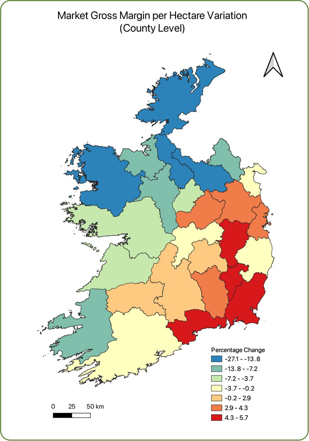
Market gross margin per hectare variation.
Our interest in the geospatial distribution of farm income relates to variation in natural capital or environmental attributes on the one hand, and the impact of agricultural activity on the other hand. In Table 6, we decompose the variation of market gross margin per hectare across all farms into between-district (geospatial area) variation and within-group variation at the sub-catchment level.9 It should be noted that between-group variation accounts for only about 9-10% of the total variation of market gross margin per hectare; it is quite low, but consistent with other findings (O’Donoghue, 2017). This reflects the greater variation between people than between places, reflecting that individual farmers makes individual decisions in relation to stocking rate, system and feed. Farmers also have different skills, efficiency and motivation.
Within and between group variation in market gross margin per hectare.
| Base | igm3 | |||
|---|---|---|---|---|
| GE(2) | Gini | GE(2) | Gini | |
| Total | 1.056 | 0.677 | 1.207 | 0.712 |
| Within | 0.960 | 1.088 | ||
| Between | 0.096 | 0.119 |
-
NB = This analysis focuses on primarily on pastoral farms;
-
The Geospatial unit is sub-catchment.
In undertaking the geospatial adjustment, we find that the simulation method captures more variation, with overall variation increasing by 14% when using the Generalised Entropy measure and 5% when using the Gini. Between area variation increases by 23% as the model improves the geospatial relationship between agricultural income and the pattern of natural capital. Within-area variability also increases but at a lower rate of 13%, given that there are environmental differences within districts as well. Combining, we find that the share of variation accounted for by between-area variation increases by 8%. Within-area variation remains the most important source of variation.
In Table 7, the statistical significance of the changes made by the simulation procedure to improve the relationship between agriculture and natural capital is reported. For all farms, the mean market gross margin per hectare falls by 5%, with the change in mean being significantly different from zero. The components of the market gross margin, output and direct costs, change by a similar percentage, maintaining the direct cost to output ratio at about 31%.
At a system level, the difference in stocking rate (intensity) and output per livestock unit (yield) on dairy farms, although significantly different from zero has the smallest change of 1% increase and a 2% decrease respectively. When combined into gross output, the changes balance out. This reflects the concentration of dairy systems on better land. The adjustment for natural capital has the highest impact for sheep farms as they occur both in upland areas and lowland areas (with very low stocking rates), with the biggest fall in intensity. This is because Both the intensity and the yield of cattle farms fall by respectively 5% and 4%.
Statistical significance of changes in Farm Market Gross Margin per hectare and its components.
| Sampled | Simulated | |||||
|---|---|---|---|---|---|---|
| LB | UB | Mean | Mean | Ratio Simulated: Sampled | Statistically Different | |
| All Farms | ||||||
| Market Gross Margin per Ha | 964 | 980 | 972 | 926 | 0.95 | 1 |
| Market Gross Output Per Ha | 1398 | 1418 | 1408 | 1336 | 0.95 | 1 |
| Farm Direct Costs per Hectare | 434 | 439 | 437 | 409 | 0.94 | 1 |
| Dairy Farms | ||||||
| Dairy Livestock Units per Ha | 1.83 | 1.85 | 1.84 | 1.87 | 1.01 | 1 |
| Dairy Gross Output per Livestock Units | 1858 | 1869 | 1864 | 1822 | 0.98 | 1 |
| Cattle Farms | ||||||
| Cattle Livestock Units per Ha | 1.33 | 1.34 | 1.33 | 1.26 | 0.95 | 1 |
| Cattle Gross Output per Livestock Units | 565 | 568 | 567 | 541 | 0.96 | 1 |
| Sheep Farms | ||||||
| Sheep Gross Output per Livestock Units | 1.59 | 1.60 | 1.59 | 1.38 | 0.87 | 1 |
| Farm Direct Costs per Hectare | 464 | 469 | 466 | 441 | 0.95 | 1 |
-
NB = LB stands for Lower Bound and UB for Upper Bound;
-
The Lower Bound represents the minimum level of gross output, gross margin, direct costs, etc. that farms have within the simulation, while the Upper Bound represents the maximum level of gross output, gross margin, direct costs, etc. The "Statistically Different" column with a value of 1 represents that the change in mean is significantly different from zero and has a probability of less than 5% of being random in terms of the mean being different from zero.
5. Discussion and conclusion
This study develops a modelling framework to improve the capacity to incorporate the heterogeneity of agricultural systems associated with local natural capital characteristics, in geospatial microsimulation models. Existing farm geospatial microsimulation models do not directly factor in natural capital (agronomic and environmental) variables and as result have a tendency to under-estimate geospatial heterogenity, which is an important element influencing costs and output. The modelling framework is then utilised to investigate the impact of natural capital on farm market gross margin.
In order to account for the geospatial heterogeneity of natural capital, we estimated an income generation model that incorporated physical capital, human capital and natural capital. Once the farm data are sampled in accordance with administrative data-based geospatial control totals, the sampled distribution was adjusted to account for the local natural capital characteristics by adjusting each component of the market output and costs. As the new geospatial distribution of natural capital characteristics is worse than the distribution within the survey, this adjustment has a tendency to reduce average incomes, reflecting the purpose and design of the farm survey used (which focuses on the representativity of output and not place). The results show the lowest incomes occur in West, North West or Border under either measure. This reflects both the fact that lower production systems locate in this area due to the poor agronomic condition (sample) and due to the relative difference in extent (simulated). The highest incomes occur in the South and Mid-West, consistent with findings in others studies. The biggest adjustments at county level occur in terms of growth 11% (Waterford in the SW) to a fall of 23% (Leitrim in the NW). In general, the counties in the East, Midlands and South East have the highest adjustment, with the North-West have the biggest reduction, consistent with grazing season length.
Decomposing the variation in income between- and within-districts, the majority of income variation occurs within-area, reflecting preferences, skills and attributes of farms and some differences in within-area natural capital. However, adjusting for heterogeneity in natural capital increases the total variation and in particular, between-area variation. The change in mean incomes resulting from this approach was statistically significant both in total and for individual income components, with the biggest changes occurring for sheep farms that are located on a variety of different land types and the smallest changes on dairy farms which are more likely to be concentrated on good land.
This paper contributes to the literature on agricultural and environmental modelling through the development of the capacity to incorporate natural capital. The paper also contributes to the field of geospatial microsimulation modelling through the advancement of modelling capacity by highlighting the importance of incorporating natural capital conditions and extent in the analysis of farm incomes and developing for its incorporation. Improving the relationship between agriculture and the local environment in economic models has the added benefit of usability for other purposes which rely on this relationship, such as analysis of environment improvement measures on farms and supporting policy frameworks. In order to enhance the model in the future by controlling the uncertainty of distributions of variables, Confidence Intervals could be used to offer more informative way to interpret results (Rahman, 2017; Veroniki et al., 2016). However, the two-stage process of sampling and calibration makes it difficult, while the scale makes it quite a computation challenge.
Improved consistency between agricultural attributes and natural local capital drivers allows for policy analyses of measures to improve the environmental footprint of agriculture. It is also useful in understanding the local economic drivers of land use change to (for example) forestry and improves our understanding of the contribution of agriculture to rural development. This methodology is scalable as the Irish FADN data used in this paper are available in other countries and similar geospatial datasets exist in many countries. However, it does rely on geo-referenced farm survey data and on the release of geo-referenced farm survey data for research purposes.
Footnotes
1.
2.
3.
4.
Björklund and Merilä, 1997 use a similar decomposition method but instead use the I0, Theil L and I1 Theil T indices.
5.
A standard output of €8,000 represents the equivalent of 6 dairy cows, 6 hectares of wheat or 14 suckler cows.
6.
This total depends upon how the NFS is weighted.
7.
The ANC scheme provides payments to people farming land in designated areas face significant hardships from factors such as remoteness, difficult topography, climatic problems and poor soil conditions. https://www.gov.ie/en/service/13d971-areas-of-natural-constraint-scheme.
8.
It should be noted that while the farms are consistent with the distribution of farms, they are not actual farms from the administrative data, but rather farms sampled from the actual NFS. The clone farms to have a geospatial and distributional pattern consistent with the administrative data.
9.
The algorithm was unable to process the analysis at the more disaggregated townland level.
Appendix A
Regression model of market gross margin per hectare as a function of natural capital variables.
| Explanatory Variables | Coef. | Std. Err. | t | Mean (Survey Data) | Mean (SMILE-GIS) |
|---|---|---|---|---|---|
| Acid Brown Earth 70% | 0.3 | 0.3 | 0.92 | 0.006 | 0.000 |
| Acid Brown Earth 70% (Coarse texture) | 0.4 | 0.3 | 1.31 | 0.008 | 0.000 |
| Acid Brown Earth 75% | 0.5 | 0.2 | 2.05 | 0.040 | 0.000 |
| Acid Brown Earth 90% | 1.2 | 0.4 | 2.73 | 0.011 | 0.000 |
| Basin Peat 100% | -0.6 | 1.5 | -0.41 | -0.010 | 0.000 |
| Blanket Peat (Low level) 100% | -0.1 | 0.4 | -0.28 | -0.001 | 0.000 |
| Brown Podzolic 60% | 0.1 | 0.2 | 0.61 | 0.016 | 0.000 |
| Brown Podzolic 80% | 0.2 | 0.4 | 0.49 | 0.007 | 0.000 |
| Degraded Grey Brown Podzolic 50% | -0.5 | 0.3 | -1.68 | -0.014 | 0.000 |
| Gley 50% | -0.3 | 0.3 | -1.08 | -0.011 | 0.000 |
| Gley 60% | 0.2 | 1.5 | 0.13 | 0.002 | 0.000 |
| Gley 75% | 0.4 | 0.2 | 1.51 | 0.024 | 0.000 |
| Gley 80% | 0.1 | 1.5 | 0.08 | 0.002 | 0.000 |
| Gley 90% | -0.4 | 1.4 | -0.29 | -0.019 | 0.000 |
| Grey Brown Podzolic 60% | -0.1 | 0.3 | -0.33 | -0.004 | 0.000 |
| Grey Brown Podzolic 70% | 0.2 | 0.3 | 0.88 | 0.011 | 0.000 |
| Grey Brown Podzolic 75% | 0.3 | 0.3 | 1.01 | 0.009 | 0.000 |
| Grey Brown Podzolic 80% | 0.5 | 0.3 | 1.64 | 0.017 | 0.000 |
| Island not surveyed | -0.9 | 0.4 | -2.26 | -0.011 | 0.000 |
| Lithosols and Outcropping Rock 70% | 0.8 | 0.2 | 3.57 | 0.084 | 0.000 |
| Minimal Grey Brown Podzolic 70% | 0.4 | 0.2 | 1.48 | 0.026 | 0.000 |
| Peaty Gley 70% | -1.1 | 0.3 | -4.18 | -0.047 | 0.000 |
| Peaty Podzol 75% | -1.2 | 0.5 | -2.65 | -0.010 | 0.000 |
| Podzol 70% | 0.4 | 0.7 | 0.59 | 0.001 | 0.000 |
| Distance to Sea | 0.0 | 0.0 | -1.53 | -0.112 | 0.000 |
| Average Temperature | -0.1 | 0.0 | -5.09 | -1.144 | 0.000 |
| Average Rainfall | 0.0 | 0.0 | -5.7 | -1.673 | 0.000 |
| Flat to Undulating Lowland (Mainly dry | -0.3 | 0.2 | -1.11 | -0.091 | 0.000 |
| Flat to Undulating Lowland (Mainly wet | 0.4 | 1.4 | 0.26 | 0.033 | 0.000 |
| Hill | 0.0 | 0.3 | 0.09 | 0.002 | 0.000 |
-
Source: Teagasc National Farm Survey and Simulation Model of the Irish Local Economy.
Gross output estimation.
| Dep var | Dairy | Dairy | Cattle | Cattle | Sheep | Sheep | Cereal |
|---|---|---|---|---|---|---|---|
| Livestock Units/Ha | Output per livestock unit | Livestock Units/Ha | Output per livestock unit | Livestock Units/Ha | Output per livestock unit | Output per livestock unit | |
| Obs | 4966 | 4957 | 13,933 | 13,845 | 4860 | 4772 | 2987 |
| R2 | 0.4225 | 0.3841 | 0.5157 | 0.2666 | 0.5976 | 0.1891 | 0.2276 |
| Price | 0.000045*** | 0.0001*** | 0.0001*** | ||||
| Fertiliser per ha | 0.0815*** | 0.0783*** | 0.2295*** | 0.033* | 0.2196*** | ||
| Purchased concentrate per Ha | 0.1525*** | 0.0988*** | 0.0147* | 0.0981*** | |||
| Share of enterprise area usage | -0.2927*** | -0.3804*** | -0.125*** | ||||
| Stocking rate for the enterprise | -0.0812*** | -0.1345*** | -0.2149*** | -0.0513** | |||
| Labour (Log) | 0.0542*** | -0.0106 | 0.0794 | 0.0419*** | 0.1001*** | 0.0829*** | 0.0172 |
| Age (Log) | -0.024*** | -0.0122 | -0.0129** | -0.0015 | 0.0007 | 0.0267 | -0.0347 |
| Has an off-farm job | -0.0109 | 0.0139 | -0.0143 | -0.01 | -0.0171 | ||
| Farm size (Log) | -0.132*** | 0.0565*** | -0.1142*** | 0.028 | |||
| Has forestry | -0.0259 | -0.0221 | -0.0499 | 0.1501*** | |||
| Extension service | -0.0055 | 0.0077 | 0.0067 | 0.0289*** | -0.0015 | 0.0035 | 0.0052 |
| Agri-environmental Sch | 0.0121* | 0.0129** | 0.0077 | 0.0001 | -0.018* | 0.0325* | 0.021 |
| Constant | -22.671*** | -5.7243*** | -6.2127*** | 19.4944*** | -0.8441*** | 14.5525 | 7.0117*** |
| Sigma u | 0.1798 | 0.1936*** | 0.2523*** | 0.3014*** | 0.3075*** | 0.4936*** | 0.4378*** |
| Sigma e | 0.1329 | 0.1343*** | 0.179*** | 0.3293*** | 0.2426*** | 0.4209*** | 0.3392*** |
| Rho | 0.6466 | 0.6753 | 0.6651 | 0.4558 | 0.6164 | 0.5791 | 0.6249 |
-
Source: O’Donoghue (2017).
References
-
1
Building a dynamic spatial microsimulation model for IrelandPopulation, Space and Place 11:157–172.https://doi.org/10.1002/psp.359
-
2
Why some measures of fluctuating asymmetry are so sensitive to measurement error.In Annales Zoologici FenniciFinnish Zoological and Botanical Publishing Board 34:133–137.
-
3
Wage discrimination: reduced form and structural estimatesThe Journal of Human Resources 8:436.https://doi.org/10.2307/144855
-
4
Decomposable income inequality measuresEconometrica: Journal of the Econometric Society 47:901–920.https://doi.org/10.2307/1914138
-
5
The Changing Structure of Irish Farming: Trends and Prospects, Vol 1, Rural Economy Research SeriesDublin: Teagasc.
- 6
- 7
- 8
- 9
-
10
Labor Market Institutions and the Distribution of Wages, 1973-1992: A Semiparametric ApproachEconometrica 64:1001–1044.https://doi.org/10.2307/2171954
-
11
A framework for classifying and quantifying the natural capital and ecosystem services of soilsEcological Economics 69:1858–1868.https://doi.org/10.1016/j.ecolecon.2010.05.002
-
12
The impact of human activities on natural capital and ecosystem services of natural pastures in North Xinjiang, ChinaEcological Modelling 225:28–39.https://doi.org/10.1016/j.ecolmodel.2011.11.006
- 13
-
14
Agronomic, economic, and environmental performance of nitrogen rates and source in Bangladesh’s coastal rice agroecosystemsField Crops Research 241:107567.https://doi.org/10.1016/j.fcr.2019.107567
-
15
Spatial Microsimulation for Rural Policy AnalysisThe SMILE model: Construction and calibration, Spatial Microsimulation for Rural Policy Analysis, Teagasc, Dublin, Advances in Spatial Science, 10.1007/978-3-642-30026-4.
-
16
How current environmental and weather conditions affect time critical decision making on irish dairy farmsInternational Journal of Agricultural Management 7:1–9.
-
17
Natural capital: assets, systems, and policiesOxford Review of Economic Policy 35:1–13.https://doi.org/10.1093/oxrep/gry027
-
18
Modelling habitat conservation and participation in agri-environmental schemes: A spatial microsimulation approachEcological Economics 66:258–269.https://doi.org/10.1016/j.ecolecon.2008.02.006
-
19
A spatial micro-simulation analysis of methane emissions from Irish agricultureEcological Complexity 6:135–146.https://doi.org/10.1016/j.ecocom.2008.10.014
-
20
Building a static farm level spatial microsimulation model for rural development and agricultural policy analysis in IrelandInternational Journal of Agricultural Resources, Governance and Ecology 8:282–299.https://doi.org/10.1504/IJARGE.2009.026230
-
21
Modeling of natural and social capital on farms: Toward useable integrationEcological Modelling 356:1–13.https://doi.org/10.1016/j.ecolmodel.2017.04.010
- 22
-
23
AccessedLPIS, https://en.wikipedia.org/wiki/Land-parcel_identification_system, Accessed, 15 September 2014.
-
24
Yield Stability in Winter Wheat Production: A Survey on German Farmers’ and Advisors’ ViewsAgronomy 7:45.https://doi.org/10.3390/agronomy7030045
-
25
Examining access to GP services in rural Ireland using microsimulation analysisArea 40:354–364.https://doi.org/10.1111/j.1475-4762.2008.00844.x
-
26
Male-Female Wage Differentials in Urban Labor MarketsInternational Economic Review 14:693–709.https://doi.org/10.2307/2525981
-
27
The Spatial Relationship between Economic Activity and River Water Quality (Economics Working Paper No. 163)Galway: Department of Economics, National University of Ireland.
-
28
Spatial Microsimulation for Rural Policy AnalysisShort and medium-term projections of household income in ireland using a spatial microsimulation model, Spatial Microsimulation for Rural Policy Analysis, Springer Science & Business Media.
-
29
Spatial Microsimulation for Rural Policy AnalysisThe SMILE model: construction and calibration, Spatial Microsimulation for Rural Policy Analysis, Springer-Verlag, 10.1007/978-3-642-30026-4.
-
30
Spatial Microsimulation Modelling: A Review of Applications and Methodological ChoicesInternational Journal of Microsimulation 7:26–75.https://doi.org/10.34196/ijm.00093
-
31
Farm-Level Microsimulation Modelling177–214, Farm-Level Income Generation Microsimulation Model, Farm-Level Microsimulation Modelling, Palgrave Macmillan, p, 10.1007/978-3-319-63979-6.
-
32
The Agri-Environmental Knowledge Innovation System for Water Quality Improvement (No. 276232)European Association of Agricultural Economists.
-
33
The spatial impact of rural economic change on river water qualityLand Use Policy 103:105322.https://doi.org/10.1016/j.landusepol.2021.105322
- 34
-
35
Small area housing stress estimation in Australia: Calculating confidence intervals for a spatial microsimulation modelCommunications in Statistics - Simulation and Computation 46:7466–7484.https://doi.org/10.1080/03610918.2016.1241406
-
36
Developing alternative income generation activities reduces forest dependency of the poor and enhances their livelihoods: the case of the Chunati Wildlife Sanctuary, BangladeshForests, Trees and Livelihoods 26:256–270.https://doi.org/10.1080/14728028.2017.1320590
-
37
Using microsimulation to maximise scarce survey data: applications for catchment scale modelling and policy analysisEnvironmental Modeling & Assessment 17:399–410.https://doi.org/10.1007/s10666-011-9300-4
-
38
An evaluation of statistical matchingProceedings of the American Statistical Association Section on Survey Research Methods. pp. 128–132.
-
39
The class of additively decomposable inequality measuresEconometrica 48:613–625.https://doi.org/10.2307/1913126
-
40
The effect of decoupling on farming in Ireland: a regional analysisIrish Journal of Agricultural and Food Research 1:13.
- 41
-
42
Pushing it to the edge: extending generalised regression as a spatial microsimulation methodInternational Journal of Microsimulation 3:23–33.https://doi.org/10.34196/ijm.00036
-
43
A review of spatial microsimulation methodsInternational Journal of Microsimulation 7:4–25.https://doi.org/10.34196/ijm.00092
-
44
Spatial microsimulation: developments and potential future directionsInternational Journal of Microsimulation 11:143–161.https://doi.org/10.34196/ijm.00176
-
45
Population Change and Impacts in Asia and the Pacific107–120, Using Spatial Microsimulation to Derive a Base File for a Spatial Decision Support System, Population Change and Impacts in Asia and the Pacific, Singapore, Springer, p.
- 46
-
47
Determinants of off-farm income and its local patterns: A spatial microsimulation of Dutch farmersJournal of Rural Studies 31:55–66.https://doi.org/10.1016/j.jrurstud.2013.02.002
-
48
Methods to estimate the between-study variance and its uncertainty in meta-analysisResearch Synthesis Methods 7:55–79.https://doi.org/10.1002/jrsm.1164
-
49
Statistics for Data Science and Policy Analysis283–304, Using a spatial farm microsimulation model for australia to estimate the Impact of an external shock on farmer incomes, Statistics for Data Science and Policy Analysis, Singapore, Springer, p, 10.1007/978-981-15-1735-8.
-
50
Assets, activities and income generation in rural Mexico: factoring in social and public capital ⋆Agricultural Economics 27:139–156.https://doi.org/10.1111/j.1574-0862.2002.tb00112.x
-
51
Modeling vegetation coverage and soil erosion in the Loess Plateau Area of ChinaEcological Modelling 198:263–268.https://doi.org/10.1016/j.ecolmodel.2006.04.019
-
52
The irish land-parcels identification system (LPIS)–experiences in ongoing and recent environmental research and land cover mappingBiology and Environment 116B:53–62.https://doi.org/10.1353/bae.2016.0025
Article and author information
Author details
Funding
The authors would like to acknowledge the support of the Teagasc Walsh Scholarship Programme.We are also grateful for funding from Science Foundation Ireland as part of the BiOrbic SFI Centre.This work has been carried out as part of the EPA INCASE (Irish Natural Capital Accounting for Sustainable Environments) project and the EPA SeQUEsTER Project (Scenarios Quantifying land Use & Emissions Transitions towards Equilibrium with Removals), funded under the EPA Research Programme 2014-2020. The EPA Research Programme is a Government of Ireland initiative funded by the Department of the Environment, Climate and Communications. It is administered by the Environmental Protection Agency, which has the statutory function of co-ordinating and promoting environmental research.
Publication history
- Version of Record published: April 30, 2024 (version 1)
Copyright
© 2024, Haydarov et al.
This article is distributed under the terms of the Creative Commons Attribution License, which permits unrestricted use and redistribution provided that the original author and source are credited.