The Italian Treasury Dynamic Microsimulation Model: Data, Structure and Validation
- Sogei S.p.A, Italy
- Department of Social Policy and Intervention and Institute for New Economic Thinking, United Kingdom
- Department of Economics, Management and Quantitative Methods, Italy
- Department of Political Sciences, Italy
- Economic Research Department, Italy
- Department of Economics and Law, Italy
Abstract
The Treasury Dynamic Microsimulation Model (T-DYMM) is a dynamic microsimulation model (DMM) owned by the Department of the Treasury of the Italian Ministry of Economy and Finance. One of the very few DMMs presently operating in Italy, it has been developed through three EU-funded research projects, spanning from 2009 to 2021. The present article is intended to provide a general and comprehensive description of T-DYMM. The model, based on the AD-SILC dataset, which matches administrative and survey data, delivers long-term simulations and is divided into five modules: demographic, labour market, pension, wealth and tax-benefit. The last two contain the most relevant novelties of the present version of T-DYMM. The broad aim of the model is to provide long-term analyses of the Italian social security system, with a focus on pension and social protection adequacy and their distributional implications.
1. Introduction
The Treasury Dynamic Microsimulation Model (T-DYMM) is a dynamic microsimulation model (DMM) owned by the Department of the Treasury of the Italian Ministry of Economy and Finance. It has been developed through a series of three research projects financed by the European Commission, spanning from 2009 to 2021. The first release of T-DYMM benefited largely from the experience of MIDAS-IT, a DMM developed by the ISAE (Istituto di Studi e Analisi Economica), which in turn drew its main features from MIDAS Belgium (Dekkers and Belloni, 2009) and the work of Gijs Dekkers, to which T-DYMM is still strongly indebted and connected. The second and third versions of T-DYMM have vastly expanded both the model structure and the dataset, as well as moved the model to its current platform, Liam 2.0 (de Menten et al., 2014).
Within the framework of research on microsimulation modelling, and taking as a reference the classifications put forward in O’Donoghue (2001), T-DYMM is a DMM that simulates life cycle events for the entire population – it is hence a population model, rather than a cohort model – uses a closed population approach,1 treats time as a discrete – not a continuous – variable, employs alignment procedures for a number of dimensions and uses sorting techniques based on regressions estimated externally (Li and O’Donoghue, 2014).
T-DYMM aims at providing long-term analyses of the Italian social security system, with a focus on pension and social protection adequacy and their related distributional implications. The model is one of the very few DMMs presently operating in Italy. It is differentiated from IrpetDin (Maitino et al., 2020) and LABSim (Bronka and Richiardi, 2022) by its comprehensiveness in terms of simulated events and policies and its extensive use of highly detailed administrative data. It is composed of five sequential simulated modules: demographic, labour market, pension, wealth and tax-benefit. Amongst the latest additions to T-DYMM are the expansion of the Tax-Benefit module, which allows for the in-model calculation of the vast majority of national-level direct taxes and benefits – LABSim integrates tax-benefit rules indirectly through its linkage with EUROMOD (Sutherland and Figari, 2013), while IrpetDin does not encompass such a module – the inclusion of an international Migration submodule and of a Wealth module. At present, the inclusion of the Wealth module is a peculiar feature of T-DYMM. Indeed, a correct simulation of the mechanisms of transmission and accumulation of wealth is crucial in inequality and poverty analyses.
The present paper is intended to provide a general and comprehensive description of the latest version of T-DYMM (third release). In the following section, we describe the data employed, focusing on the steps undertaken to build our dataset, named ‘AD-SILC’, and how we derived the starting sample for the simulations. In the third section, we explore the model structure and main processes. Finally, we validate the model in its baseline version by comparing model outputs to historical external data and observing long-term patterns produced by the simulations. The last section concludes the study and discusses possible expansions of the model.
2. Data and starting sample
2.1. AD-SILC dataset
The core of T-DYMM’s dataset is obtained by linking data from the Italian component of the European Union Statistics on Income and Living Conditions (IT-SILC) survey, administered in Italy by the Italian National Institute of Statistics (ISTAT), with administrative data from the Italian National Institute of Social Security (INPS). The merging procedure is conducted through individual tax codes (codici fiscali) that are subsequently anonymised. The merged dataset, named ‘AD-SILC’, can be employed for a number of uses: i) to analyse historical dynamics (e.g. within the labour market); ii) to estimate transition probabilities to be included in T-DYMM; and iii) to derive the starting sample for the simulations. AD-SILC is an unbalanced panel dataset that, in its current version, comprises the information contained in all IT-SILC waves from 2004 to 2017 and in the INPS archives (for the linked individuals). From IT-SILC, we derive longitudinal data (respondents are followed for up to four years) on socio-economic characteristics for a total of 254,212 individuals; from INPS, we derive longitudinal data on pensions (disability, old age, survivor, etc.) and working history (occupational status, income evolution, contribution accrual, etc.), for a total of 6,182,926 individual-year observations over the period from 1922 to 2018. In addition to the IT-SILC and INPS data, the latest version of AD-SILC includes information from tax returns and the Cadastre collected by the Department of Finance of the Italian Ministry of Economy and Finance (DF) for the IT-SILC waves corresponding to 2010, 2012, 2014 and 2016 (the reference period for tax records refers to the year before the interview, while INPS data are aligned with interview years). Tax return data are used to correct the information contained in INPS data concerning labour income from self-employment.2 Housing wealth information is derived from the Cadastre and tax returns, whereas information on financial wealth and liabilities is retrieved through a statistical matching procedure from the 2016 Survey on Household Income and Wealth (SHIW) after applying a specific correction for financial wealth to take into account a well-documented under-reporting issue.3 With these last two data sources, we were able to build a rich dataset on household wealth, laying the ground for the Wealth module.
2.2. T-DYMM’s starting sample
The starting sample for the simulations is set in 2015 and derived from a single extract of AD-SILC, i.e. the 2016 IT-SILC wave – composed of 48,316 individuals and 21,325 households – linked with all the aforementioned administrative data for the 2015 year and imputed financial wealth amounts from the SHIW survey for 2016. Before running the simulations, we apply a weight calibration procedure in order to improve the overall representativeness of the series of dimensions we are interested in and bring back relevant socio-demographic characteristics to 2015.4 This procedure is similar to the calibration performed for static microsimulation models. The calibration is carried out on the IT-SILC weights provided in the 2016 wave (Eurostat, 2017) and ensures that individuals belonging to the same household have the same calibrated weight (integrative calibration). It is carried out thanks to the sreweight Stata command (Pacifico, 2014), which replicates the algorithmic solution put forward by Creedy and Tuckwell (2004) in the context of Deville and Särndal (1992)’s raking techniques. We constrain for the same characteristics employed by ISTAT in the calibration of the IT-SILC weights and we add several dimensions relevant to the scopes of our analyses (e.g. distribution of the population by gender and one-year age groups; distribution of individuals with retirement income by gender and type of pension; distribution of in-work individuals by employment status; and distribution of individuals with gross income subject to the personal income tax by income group). Subsequent to the weight calibration, we expand the sample by multiplying individuals by calibrated weights. We then draw with replacement 100 samples of 100,000 households and select the best-fitting sample that minimises the difference between calibrated and external totals. As a result, the starting sample contains 238,431 individuals. We refer to this sample as T-DYMM’s base year sample, which is the starting point of all our simulations. This procedure is a common practice in dynamic microsimulation studies and overcomes the difficulties related to the use of alignment methods, although alternative strategies that do not involve the expansion of the sample have also been proposed (Dekkers and Cumpston, 2012).
2.3. Exogenous data and alignments
Exogenous data are used to align a number of patterns within the simulations. The use of alignment procedures is generally regarded as a fundamental step towards the delivery of reliable projections, although the debate on which variables should be aligned and how extensive the alignments should be is far from settled (Baekgaard, 2002; Li and O’Donoghue, 2014). Besides using alignments for dimensions that cannot be produced within the model (e.g. fertility and mortality rates, gross domestic product (GDP) growth, inflation, etc.), in institutional models such as T-DYMM it may be preferable to ensure that certain macroeconomic dynamics that could be generated within the model (e.g. employment rates) stay in line with third-party projections and let the model focus (for instance) on distributional concerns. Alignments may then be employed to simulate sensitivity scenarios. Table 1 lists the main processes in T-DYMM by use of alignment procedures, linking the corresponding module and source. Most processes in the Demographic module are aligned, while the opposite is true for all other modules.
Aligned processes in T-DYMM.
| Module | Process | Source |
|---|---|---|
| Demographic module | Fertility, mortality, immigration and emigration flows | ISTAT (historical data) and Eurostat - Europop 2019 projections |
| Education, age of exit from original household, informal and formal marriages, divorces | ISTAT and OECD (for education achievements of immigrants) | |
| Labour Market module | Employment rate, inflation growth, GDP growth, productivity growth | ISTAT (historical data) and European Commission 2022 Spring Forecasts and Working Group on Ageing Populations and Sustainability (AWG) assumptions |
| Take-up rate of unemployment benefits | INPS | |
| Quota of permanent public employees | ISTAT | |
| Pension module | Number of disability allowances and incapacity pensions | INPS |
| Enrolment in private pension plans | Italian Supervisory Authority on Pension funds (COVIP) | |
| Wealth module | Households that pay rent | Department of Finance |
| Returns on financial and housing assets | European Commission 2022 Spring Forecasts and AWG assumptions, Italian Housing Observatory (Osservatorio del Mercato Immobiliare, OMI) and Standard & Poor’s (S&P) 500 | |
| Houses sold and bought, average propensity to consume | ISTAT | |
| Tax-Benefit module | Beneficiaries of selected tax expenditures and substitute tax regimes | Department of Finance |
| Take-up rates of specific social assistance measures | INPS |
3. Model structure
The present section illustrates the current structure of the baseline version of T-DYMM. The model is divided into five modules, as shown in Figure 1, and operates sequentially. In the present version of the model, the starting sample is set in 2015, and simulations run on an annual basis from 2016 until 2070 (the projection horizon of the 2021 Ageing Report by the European Commission). The organisation in modules is logical and does not strictly represent the sequence of processes that the model solves.5 The modular structure and set of estimates underlie the results validated in Section 4. The legislation simulated in the model is updated to 2022.
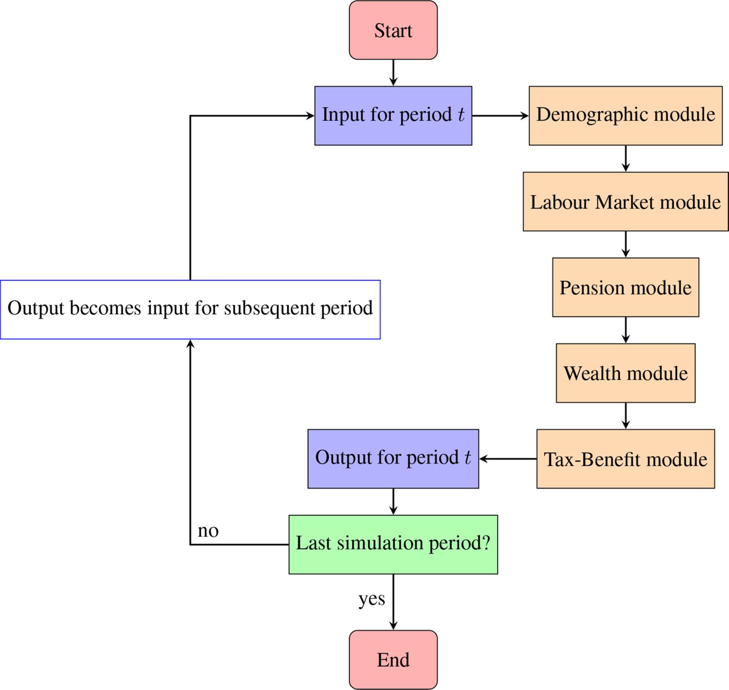
Modular structure of T-DYMM
3.1. Demographic module
The units of analysis in the model are individuals and households. In the Demographic module, the sample evolves in its components related to demographic aspects. Individuals in the sample are born, age, die, migrate, get educated, leave their households of origin, form couples and separate, become disabled.
T-DYMM is an annual model and all states are updated annually, starting with ageing. At present, death is assigned randomly according to aligned mortality rates by age and gender following the latest Europop projections. The possibility of introducing heterogeneity in mortality according to additional dimensions (marital status, income, education achievement) has been considered, as it would allow analyses on implicit distributive features of the pension system.
Fertility rates (for women between 14 and 50, by age) are aligned with the latest Europop projections. Parameters estimated via logit regressions in the AD-SILC dataset distribute the probability of having children across women by civil status, duration of marriage/cohabitation, presence of other children and employment status.
Regions and municipalities are not modelled in T-DYMM and only international migration is addressed. Considering the well-known scarcity of quality data on the international migration phenomenon, we have opted for a rather simplified modelisation of the Migration submodule in T-DYMM, which could serve as a basis for future expansions when further micro data become available. Unlike other processes in the Demographic module, migration is dealt with at the household level. We focus on three essential dimensions to define migrants: age, gender and area of birth (Italy, European Union (EU) and non-EU). We simulate immigration and emigration separately and follow Chénard (2000) and Dekkers (2015) in implementing a ‘cloning procedure’ for households using Chénard’s Pageant algorithm, which allows households to be selected in the model (to either immigrate or emigrate) while ensuring that certain individual characteristics (in our case: age, gender and area of birth) are matched. Inflows and outflows of migrants are aligned with Europop projections; education (for immigrants) and area of birth (for both immigrants and emigrants) are assumed constant (by gender and age group) according to OECD and ISTAT data, respectively. Immigrants are included as clones but lose all original characteristics of the individuals they are cloned from other than age and gender (which are aligned) and household composition; the implicit assumption is that all immigrants ‘start fresh’ when they arrive in Italy, carrying no relevant work experience with them and no pension rights. These simplifying assumptions are due to a lack of data, though they should not necessarily be looked at as excessively stringent, given the age structure of the immigrant population and the segregational features of the Italian labour market (Strozza and De Santi, 2017). As no data are available at this point to model emigrants’ behaviour once they leave Italy, they are simply deleted from the simulation; i.e. households (and individuals) are not followed in their (possibly) multiple entries/exits. Therefore, while we align the overall flows with Europop projections, we may be overestimating the incidence of the migration phenomenon on individuals.6
Each year T-DYMM assigns an individual probability of becoming disabled (‘strongly limited in daily activities on a long-term basis’, according to the EU-SILC definition) based on regression parameters estimated on the basis of AD-SILC that highlight the role of education, income and disability state at time t-1 (disability is highly persistent). Probabilities by gender and age group (nineteen age groups) are aligned with the assumptions underlying the 2021 Ageing Report.
Individuals in the model may hold elementary, lower-secondary, upper-secondary or tertiary education. Following the legislation on compulsory education in Italy, in simulation years T-DYMM assigns lower-secondary education as the lowest possible education achievement for individuals who receive their education in Italy.7 Probabilities of getting a tertiary education are assigned individually based on estimations run on the AD-SILC dataset. Due to the difficulty of attributing time-variant characteristics relative to the moment when the latest educational level was achieved, the only explanatory variables employed concern parental education, assumed to be time-invariant. Levels of education lower than tertiary are assigned randomly, while all probabilities by gender are aligned with ISTAT data. Individuals receive lower-secondary education at 16, upper-secondary (if entitled) at 19 and tertiary (if entitled) between 21 and 29 years of age according to probabilities derived from AlmaLaurea survey data.
Since T-DYMM estimates poverty and distributive indicators, income variables need to be computed at the household level to derive the household disposable income. Therefore, it is crucial that households are properly designed. Each year, young individuals still living with their parents are assigned a random probability to leave and form a new household; the latest ISTAT data on the quota of young people living with their parents (by gender) are used to align future exit flows. Young people below a given income threshold are not allowed to leave families of origin and live as independent single-member households. If they are suffering from severe disabilities, they are not allowed to form new nuclear families either.
Each year, single individuals are assigned a probability of forming a couple according to estimates based on AD-SILC and alignments from ISTAT data. Since the past few years have seen a visible and somewhat uncharacteristic decrease in the propensity to marry, we assume that the number of marriages among every 1,000 individuals will start rising again and recover, by 2029, its 2008 value. Following the progression observed in census data, we assume that every four marriages, a new informal cohabitation is established. Once individuals are selected to be coupled, they are matched according to a score that takes into account age and education differentials and a dummy returning 1 if both potential partners are employed (we are attempting to reproduce the positive ‘assortative mating’ behaviours that we observed in AD-SILC data). Each year, couples are assigned a probability of divorcing or separating (depending whether they are married or in an informal union) according to estimations on AD-SILC. The overall propensity to divorce or separate is aligned with ISTAT data. The passing of legislation on the so-called ‘fast divorce’ (divorzio breve, which has sped up divorce procedures) produced a break in the series from 2015–2016, when the number of yearly divorces doubled compared to previous years. In order to account for this and for the following gradual reduction of yearly occurrences in the 2017–2019 period, we assume that the propensity to divorce or separate will keep reducing linearly and, 10 years after the approval of the aforementioned legislation, stabilise at a rate equal to an average of pre- and post-reform values.
3.2. Labour market module
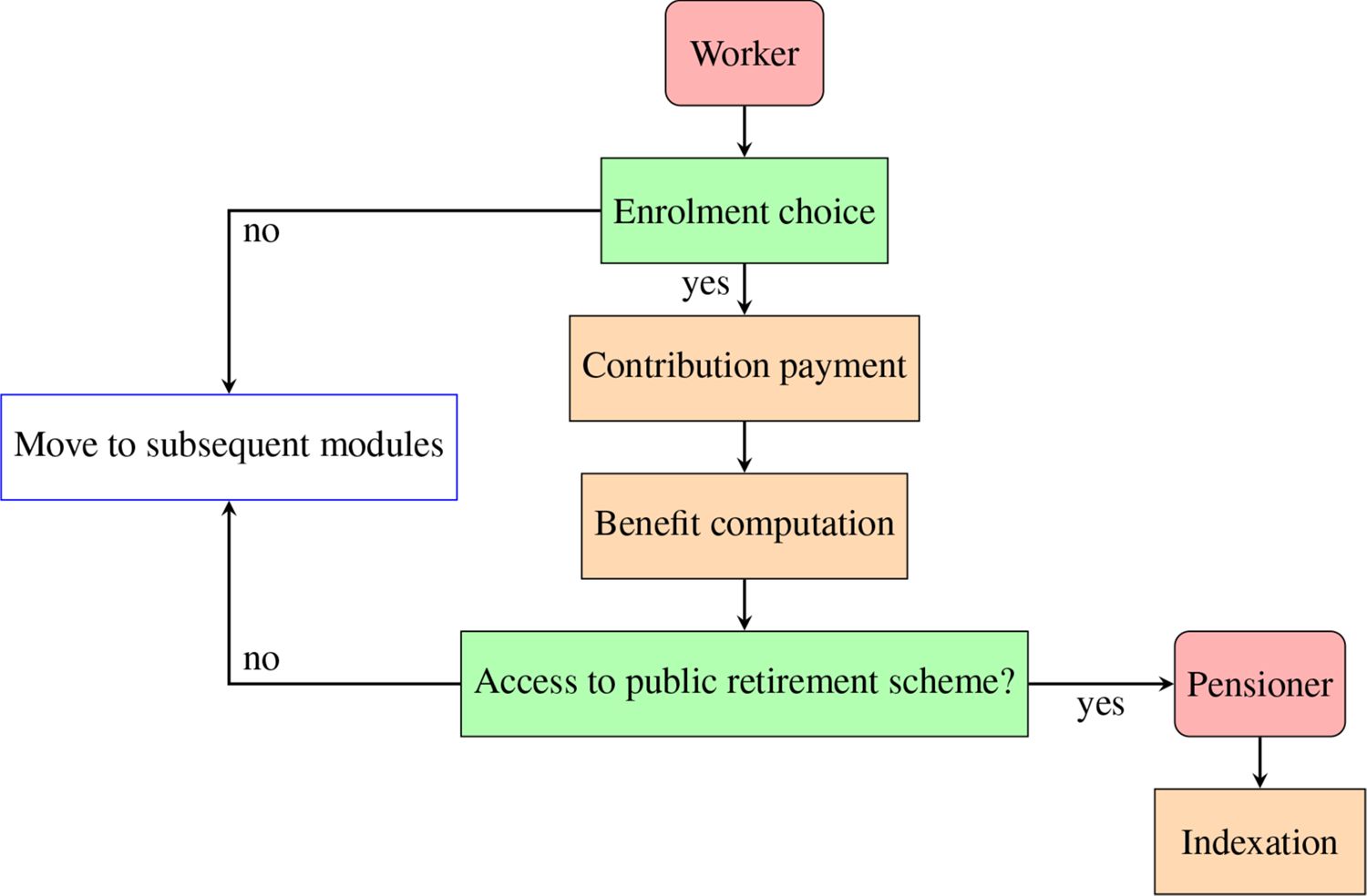
Much like the Demographic module, the Labor Market module is an essential pillar of T-DYMM, as its outputs become inputs to most other modules. On one hand, intermittent careers or low salaries will have an impact not only on the current economic status and on the access to unemployment benefits, but also on retirement prospects and on the possibility for individuals to accrue savings and wealth. On the other hand, different socio-demographic and economic determinants may influence individual careers. In T-DYMM, the Labour Market module assigns individuals to employment, simulates transitions between different employment statuses, imputes the number of months in work within the year and the corresponding level of labour income. The module is based on a sequence of nested choices, as shown in Figure 2, following probabilities estimated through a series of logistic and multinomial logistic equations. Estimates have been run on individuals recorded in AD-SILC between 15 and 80 years of age, including students and retirees. Because of their specificity, working pensioners follow separate and simplified processes compared to other workers. Among all the demographic, socio-economic and career variables present in the AD-SILC dataset, we include in our regression estimates those for which we can project the evolution over the simulation period. This allows us to account for the same degree of heterogeneity in both the regressions and the simulations.8 Below, we shall illustrate the processes included in the module, while the main regression results are reported in Appendix A3.

Structure of the Labour Market module
The first process determines whether individuals are employed, on the basis of a logit regression. As already mentioned, employment rates by gender and age are aligned, following the macroeconomic assumptions underlying the 2021 Ageing Report. People who are not employed are instead assigned to ‘out-of-work’ statuses, which include individuals receiving incapacity pensions, unemployment benefits, or those in other forms of unemployment or inactivity.
For those working, a multinomial logit assigns the probabilities of different contractual arrangements. We grouped individuals into five working categories using INPS data: open-ended employees, fixed-term employees, professionals, self-employed and atypical workers (i.e. co.co.co. according to the Italian acronym). In the model, workers are allowed to have one job per year, although roughly 10% of the observations in AD-SILC hold multiple job spells. For those individuals, we must identify an annual main employment category. To define the most representative work for a given period, we compare the multiple jobs performed within a year and order them according to the following criteria: level of earnings, duration of the working relationship, level of social security contributions accrued, latest job position held within the year and level of employment stability (e.g. open-ended contracts are more stable than fixed-term contracts). As previously mentioned, ad hoc estimates are run to assign working categories to working pensioners. Because of the smaller sample, they are not split by gender and are not allowed to work as public employees, who represent a negligible fraction of working pensioners in the data.
For non-retired employees, further logit regressions determine who works in the public or private sector and who works part-time or full-time. As public employment meets the need for providing public services, which, in turn, depend on the size of the population (at parity of public services provided), the share of open-ended public employees is kept constant at 2015 levels. The relative share of other working categories over total employment in the model is not aligned.
After determining the work type, the following process assigns the number of months worked within the year. Self-employed workers, professionals and permanent employees are assumed to work all year. For the first two categories, because of the nature of the job, AD-SILC data do not allow a precise estimate of months worked to be obtained, while for open-ended employees, working for a fraction of the year is not indicative of a state of precariousness but rather a result of the fact that workers can be hired or fired at any point within the year, and not necessarily at the beginning. For all other workers (fixed-term employees and atypical workers), a logit model determines who is working for the whole 12 months. If workers are not employed for a whole year, a random-effect model estimates the number of months worked by gender.
Finally, we estimate monthly labour income via a random-effects model. We run estimations separately for each employment category simulated in the model but group together fixed and open-ended contractual arrangements for private and public employees. Keeping fixed-term and open-ended contracts together allows us to separately analyse men and women. The group of public fixed-term male employees is too small to be studied alone and must be combined with either the corresponding female group or the corresponding open-ended one. We find that the gender component is more relevant for income prospects compared with the distinction between open-ended and fixed-term arrangements. Because the model allows only one type of job per year, wages in the estimate sample are obtained as the summation of the overall labour income earned, attributed wholly to the main employment category assigned for that year. Possible amounts received as indemnities for maternity, sickness or job suspension are included. For the estimation of labour incomes for working pensioners, all employment categories are grouped and only one equation is estimated. Monthly labour income is simulated in real terms and then (when ISTAT historical data for wage growth are no longer available) aligned with labour productivity growth and the consumer price index, a rather theoretical and optimistic assumption if one looks at the limited wage growth observed in Italy in the last few decades.
3.3. Pension module
Figure 3 illustrates the structure of the Pension module in the latest version of T-DYMM, which largely draws from the experience of previous releases of the model.

Structure of the Pension module, work-related public pensions (first pillar)
Workers contribute to the first (public) pension pillar on a mandatory basis, with contribution rates set in accordance with the employment category assigned in the Labour Market module. Every year, a potential pension benefit is computed according to the pertinent pension regime.
Present contributors to the pension system can be divided into two main categories: ‘(Pure) NDC’ (contributivo puro) for workers with no seniority prior to 1996, for whom benefits are entirely calculated according to notional defined contribution (NDC) rules; ‘Mixed’ (misto), divided into i) ‘Mixed 1995’, for workers who had less than 18 years of seniority in 1995, for whom benefits are calculated according to NDC rules pro rata for all years of seniority following 1995; ii) ‘Mixed 2011’, for workers with at least 18 years of seniority in 1995, for whom benefits are calculated according to NDC rules pro rata for all years of seniority following 2011. While present contributors all compute at least a portion of their pension benefits according to NDC rules, a very consistent portion of present retirees receives a pension that was entirely calculated according to the old defined benefit (DB) rules.
After potential benefits are computed, individuals are checked for retirement eligibility. Table 2 illustrates the various modalities for accessing retirement in T-DYMM according to the Italian legislation as of 2022.9
Eligibility requirements for retirement as simulated in T-DYMM.
| Criteria | Regime | Requirements | 2022 |
|---|---|---|---|
| Old age 1 | NDC | age | 64 years |
| seniority | 20 years | ||
| amount | 2.8*assegno sociale | ||
| Old age 2 | NDC, mixed | age | 67 years |
| NDC, mixed | seniority | 20 years | |
| NDC | amount | 1.5*assegno sociale | |
| Old age 3 | NDC | age | 71 years |
| seniority | 5 years | ||
| Seniority | NDC, mixed | seniority, males | 42 years, 6 months |
| seniority, females | 41 years, 6 months | ||
| Seniority - young workers | mixed | seniority | 41 years, 12 months accrued before turning 19 |
| Seniority - Quota 100/102 | mixed | age | 62/64 years |
| seniority | 38 years |
-
Note: The assegno sociale is the social allowance for the elderly. Since 2018, age requirements are aligned with ‘Old age 2’. Concerning ‘Old age 2’ seniority requirement, 15 years suffice for workers with at least 15 years of seniority as of Dec 31, 1992. For 2022, ‘Seniority - Quota 102’ replaces ‘Quota 100’ and the age requirement rises to 64.
Age requirements for ‘Old Age 1’, ‘Old Age 2’ and ‘Old Age 3’ criteria and seniority requirements for ‘Seniority’ and ‘Seniority – young workers’ criteria are updated every two years in line with variations in life expectancy at 65 years of age, as established in 2010.10 ‘Seniority – Quota 100’ was introduced in 2019 for the 2019–2021 period, then renewed as ’Quota 102’ for 2022 (the age requirement is set at 64, 2 years more than the original ‘Quota 100’). Workers past the ‘Old Age 2’ age criterion may access a means-tested social allowance for the elderly (the so-called assegno sociale, see Section 3.5). In its present version, T-DYMM does not simulate retirement according to the so-called ‘APE’ (Anticipo pensionistico) criterion, introduced in 2017 and discontinued in 2020 after limited participation, or the ‘Opzione donna’ criterion, by which female workers belonging to the ‘Mixed’ regime may access retirement many years in advance (as of 2022, 58 years of age for employees, 59 for self-employed workers) if they choose to switch entirely to NDC computation rules. Special retirement schemes relative to specific sectors and work categories that are not simulated in the model are also excluded from the simulated legislation.
In the previous releases of T-DYMM, retirement decisions were purely deterministic: individuals accessed retirement as soon as they were entitled to. Such an assumption may seem acceptable in the present, as age requirements in Italy have raised rapidly in the past few years, especially for women. However, as NDC rules phase in, average pensions are expected to lower and a strong economic incentive to postpone retirement to increase benefits (both by increasing contributions accrued and by reducing life expectancy at retirement) will kick in. By assuming that workers retire as soon as possible, we are implicitly assigning a stronger preference to spending more time in retirement rather than getting a higher benefit to all, and when called to assess the frequently discussed policy options for early retirement, would certainly overestimate the quota of workers accessing them. A choice function that differentiates among different profiles may provide a better representation of reality. The latest version of T-DYMM offers a first attempt at this. Workers who meet eligibility requirements for retirement undergo a choice process. The choice function introduced is based on an option value model (Stock and Wise, 1990). For the structure of the model, we took inspiration from van Sonsbeek (2010), but we use the parameters estimated for Italy by Belloni and Alessie (2013). If workers meet the requirements for retirement, they will choose whether to cease or continue working. For each year between the present and the ‘maximum retirement age’ (the age requirement for the ‘Old Age 3’ criterion, presently set at 71 and subject to future increases according to changes in life expectancy), the utility of accessing retirement in the current period is confronted with the utility obtained by postponing retirement in yearly steps. Future salaries are assumed equal to the latest available salary, augmented by labour productivity and inflation growth (for each year in the future, growth values in the choice function are assumed equal to the average between period t and t-1). Individuals only consider the option of working a whole year, because in case employment is discontinued, workers will have the possibility to access retirement (seeing as they meet the requirements), regardless of the choice they made beforehand. It is therefore reasonable that individuals do not take unemployment risks into account. For every year in the cycle, there is a different hypothetical retirement age and a different first hypothetical pension, which is computed according to the hypothetical working history accrued on top of the working history already known at the time the decision is made. Utilities are computed as a weighted (by survival probability) sum of future salaries and pensions, reevaluated and discounted, and net of taxes and contributions. If the utility of accessing retirement in the current period is higher than in any other option (delay by one year, delay by two years, …, delay until the maximum retirement age is reached), retirement is accessed. Parameters exogenous to the model are i) discount rates (labour productivity and inflation, in our case); ii) risk aversion and iii) leisure preference. The parameters for risk aversion and leisure preference (by gender) are derived from Belloni and Alessie (2013). Early-retirement schemes such as ‘Quota 100’ was used to validate our retirement choice function, and the results are promising.11
Once workers access retirement, their pension is paid out, and for the following periods it is indexed to price inflation according to the pertinent legislation, which only allows full indexation to pensions below a certain threshold amount (in 2022, below 2,101.52 euros monthly). For the period 2019–2021, an ad hoc temporary reduction on pensions above 100,000 euros annually (so-called ‘pensioni d’oro’) is also in place.
Besides seniority and old-age pensions (work-related pensions), in the Pension module we also simulate the integration to a minimum amount for pensions of workers belonging to the ‘Mixed’ regime, incapacity pensions for workers that fall ill or disabled and survivor pensions. For incapacity pensions, we simulate the legislation put in place in 1984, which introduced the Assegno ordinario di invalidità, for severely disabled workers, and the Pensione di inabilità, for workers unable to work because of disability. Individual probabilities of receiving these benefits are based on regression parameters estimated on the basis of AD-SILC, which highlight the high persistency of the phenomenon and the relevance of the disability state (simulated in the Demographic module; see Section 3.1). Probabilities of receiving incapacity pensions are aligned by gender and five-year age group with INPS data available for the period 2016–2019; beyond 2019, probabilities are projected following the same logic adopted for disability probabilities.
The Pension module also comprises a submodule on private pensions. Figure 4 illustrates its structure. As opposed to what happens in the first pillar, workers participate in private plans on a voluntary basis. Individual probabilities are based on regression parameters estimated on the basis of AD-SILC, which highlight the roles of age, labour income, financial literacy, education, employment category and net wealth, and impose a high level of persistence on the phenomenon. The probability of contributing is aligned, irrespectively of age and gender, according to data from COVIP; in projection years, it is kept constant to the latest available figures. Contributors to the second pillar (fondi negoziali, collective funds) may devolve their TFR (Trattamento di Fine Rapporto, end-of-service allowance) and voluntary contributions, while for the third pillar (either fondi aperti, open funds, or piani individuali pensionistici, individual pension plans), contributions to the fund may vary yearly depending on labour income and net wealth.12 Investments in the second and third pillars produce returns that are computed following COVIP data for past periods, while they are projected based on assumptions on future portfolio compositions of pension funds and on their returns (for a description of the assumptions about various financial assets, see Section 3.4). When individuals access retirement in the public pillar, they are also assigned an annuity (if any investment is present) from the second and/or third pillar, which is henceforth indexed.
Structure of the Pension module, private pensions (second and third pillars)
3.4. Wealth module
One of the main novelties of T-DYMM is the introduction of a Wealth module that accounts for household wealth dynamics. Modelling private wealth provides a more complete picture of disposable income and households’ well-being distribution, linking these factors to the adequacy of the social security system. We define net wealth as the sum of real and financial wealth net of liabilities. House ownership is the only form of real wealth in our model, while financial wealth is divided into four categories: liquidity, government bonds, corporate bonds and stocks, which correspond to four different risk-return combinations. In the present version of the model, investors do not experience risk, as return vectors contain average values and no idiosyncratic component is simulated.
The structure of the Wealth module is based on the CAPP-DYN microsimulation model (Tedeschi et al., 2013), and illustrated in Figure 5. The processes in the module are sequential, as presented from top to bottom in the flowchart, although they are interrelated over time. For instance, the acquisition of real estate implies down-spending of financial wealth, while the opposite stands for selling. Every step of the module involves choices made at the household level that are modelled through regressions and alignments (when needed). The estimates adopted in the model are based on SHIW micro data (biennial waves in the 2002–2016 time span). We use discrete choice models (logit) for transitions (for instance buying/selling houses, making/receiving inter-generational transfers, renting second dwellings) and continuous regressions for quantities (either log levels or ratios of income or financial wealth). In Appenix A4, we illustrate the regression results underlying some of the module processes. The general criteria that guided the selection of the explanatory variables of the estimates are the economic relevance of the variables with respect to the dependent variable and the significance of the estimated coefficients.13 The two criteria did not have a hierarchical order but were combined to obtain the most reasonable result in an economic and econometric sense. As mentioned above, alignments are a key part of a DMM, and data from ISTAT and the Department of Finance have been used to this scope within the Wealth module, as we will specify below.
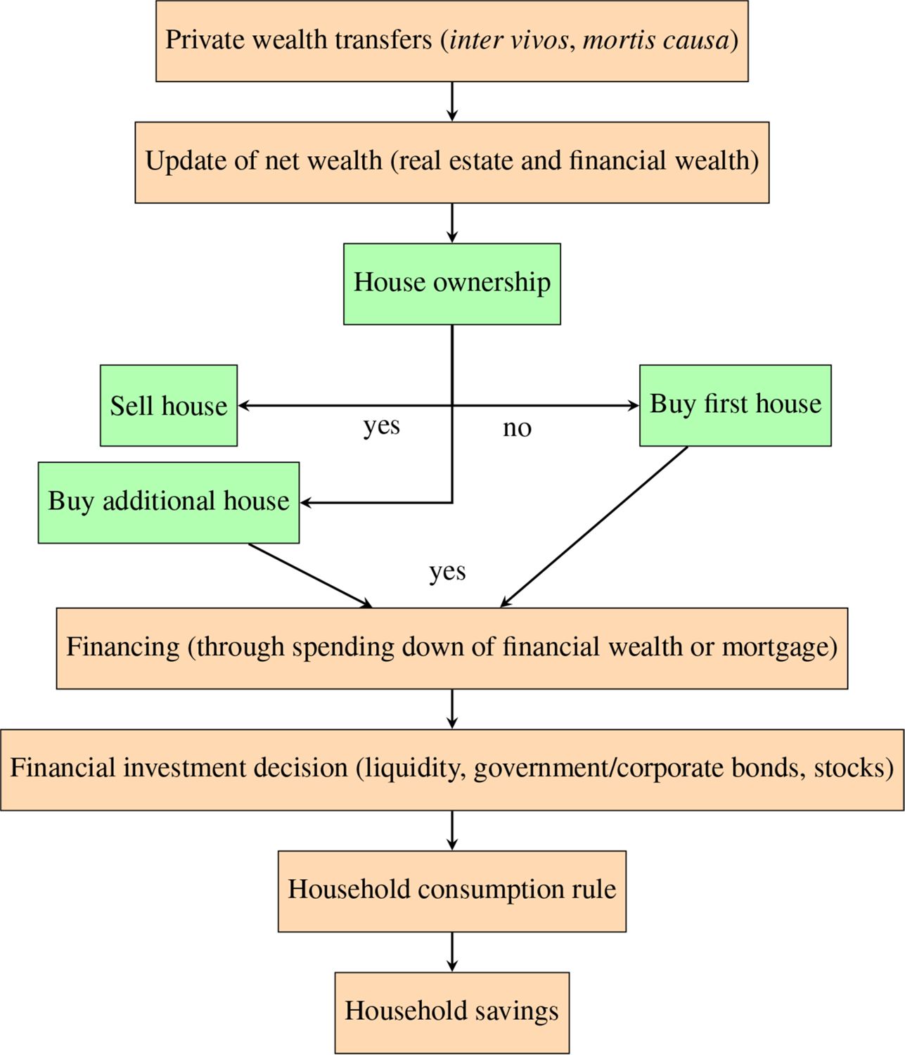
Structure of the Wealth module. Note: If individuals do not sell or buy a house, they move to financial investment decisions and subsequent processes.
The starting processes involve intergenerational transfers, inter vivos (donations) and mortis causa (inheritances). Inheritance is driven by demography in the sense that the total amount of transferred wealth equals the wealth of the deceased. Receivers are selected deterministically, as the offspring and/or married partner of the deceased, if present in the sample, or probabilistically, through regressions based on SHIW. At the start of the simulation, no individuals living outside of their original households can be linked to their parents, creating the need to simulate some inheritances in a probabilistic fashion. Inter vivos transfers are based on SHIW data on both the donor and recipient sides; the number of households who donate and receive and the related total amounts are imposed to match each other in terms of totals. Both inheritances and donations are reduced by the inheritance tax, but only if the total amount received exceeds 1 million euros, as determined by Italian legislation.
The second process updates the amount of yearly wealth. Household savings and the TFR (Trattamento di Fine Rapporto, end-of-service allowance) are summed up to the existing financial accrual, and the values of house wealth and financial wealth evolve over time depending on nominal rates of returns. House wealth evolves following inflation, assuming that the real market does not incur a significant value increase or decrease over time, while income gains follow returns data from the OMI (Osservatorio del Mercato Immobiliare, the Italian Housing Observatory) and are projected up to 2070 in accordance with the evolution of the implicit interest rate on the Italian public debt (computed in line with the European Commission methodology, following the assumptions underlying the 2021 Ageing Report). As for financial wealth, each of its components evolves differently, as sketched in Table 3. Liquidity is not updated over time, meaning that its value is eroded in real terms. For the remaining financial investments, except for government bonds, we divided returns into two components: income and capital gain. The former derives from interests on financial assets, while the latter indicates the evolution of asset values; therefore, their establishment will affect the evolution of the wealth-to-income ratio in the simulations. Government bonds are assumed to produce no capital gain in real terms (their value is updated in line with inflation), while their income gain follows the implicit rate of return on public debt. For corporate bonds and stocks, we use information from S&P 500 to derive both income and capital gain in historical periods, while for future years we use the projected implicit rate of return on public debt for the income component. For the capital gain, we attribute an extra yield, computed as the historical average return differential with respect to government bonds, kept constant from 2024 (the first year beyond the forecast horizon of the European Commission 2022 Spring Forecasts) to 2070. From the latest historical data available (2021) to 2024, a linear convergence is assumed. Finally, mortgages evolve based on the long-term (10-year Italian government bonds) interest rate for both historical and projected periods. Like the implicit rate of return on public debt, the long-term interest rate is also projected following the European Commission methodology and the assumptions underlying the 2021 Ageing Report.
Projected rate of nominal returns adopted in the Wealth module.
| Wealth component | Gain | 2016–2021 | 2022–2070 |
|---|---|---|---|
| House wealth | Income gain | OMI | Projections based on OMI |
| Government bonds | Income gain | Implicit rate of return on public debt, Italian Treasury Department | Implicit rate of return on public debt, EU Commission |
| Corporate bonds | Income gain | S&P 500 | Implicit rate of return on public debt, EU Commission |
| Capital gain | S&P 500 | Projections based on S&P 500* | |
| Stocks | Income gain | S&P 500 | Implicit rate of return on public debt, EU Commission |
| Capital gain | S&P 500 | Mark-up stocks–bonds* | |
| Mortgages | Long-term interest rate, Italian Treasury Department | Long-term interest rate, EU Commission |
-
*
For the 2022–2023 period a linear convergence is applied to ensure a smoother transition from historical data to long-term assumptions.
Every household has a probability of buying and selling a house based on regressions estimated on SHIW data. Every simulation year, the number of houses bought equals the number of houses sold, and these values are aligned with the national statistics from ISTAT (historical values for 2016–2021, then the 2021 value is kept constant over time). The values of the houses sold are deterministically computed within the model, whereas the values of the houses bought are computed through regressions. House acquisition is financed through down-spending of financial wealth, the accrued TFR (70% of the total, in line with the pertinent legislation) and residually through mortgages (which are the only form of liability in the model). The values of new mortgages cannot exceed 60% of household income. An extra process that is connected to house property is the event of renting, which constitutes a further source of income for owners and an expenditure for households that are not house owners. The choice of whether to rent real estate in excess (renting the first house is not allowed in T-DYMM) is modelled with a regression based on AD-SILC data (specifically, the information contained in tax returns allows us to study this choice). The households that do not own a house may or may not live in rented houses (the possibility of loan to use is taken into account). To model this circumstance, we use a regression based on SHIW data. The amounts of rent paid out are simulated as a share of the dwelling’s value. The number of households who pay rent equals the number of households who receive rents (closed population approach), and the total amount of rent paid equals the total amount of rent received.
As said above, T-DYMM simulates four different types of financial activities. Financial investment decisions are modelled in two steps: we first simulate ownership and then the amount owned. We model in a probabilistic fashion the choice of whether to invest in government bonds, corporate bonds or stocks through dynamic regressions based on SHIW data. In order to estimate the dynamic relationship between ownership at time t and t-1 and control for the initial conditions problem, we check for the value of the dichotomous dependent variable in the first year of observation (whether they owned that class of financial activity in 2010) and we average all time-varying variables, following the approach of Wooldridge (2005). In the simulation, we do not use the coefficients for initial conditions and averages, but we consider them good instruments for improving the precision of coefficients of the lagged dependent variable. The breakdown of total financial wealth into the various asset groups is obtained through regressions based on SHIW data, with the ratio of the asset amount over the total as the dependent variable.
The last process in the Wealth module is the household consumption decision. This process is one of the most relevant since household savings flow into the household budget the following year in the form of financial wealth. At the end of the simulation period, every household is endowed with an amount of disposable income, and the model attributes them a certain level of consumption that may or may not exceed the household disposable income; in the former case, the household will use its financial wealth as a supplementary source to finance its expenditure. Consumption levels are determined through a panel regression based on SHIW data covering the period 2002–2016, where the dependent variable is the logarithm of consumption. We adopt a fixed effects estimator, and the estimated correlation between the vector of explanatory variables and the unobserved time-invariant residual is included in the simulation.
The results of the regression estimates highlight an issue related to the difference between micro data and macro aggregates on consumption and savings rate. As is well known in the literature (Cifaldi and Neri, 2013), the discrepancy between the savings rate obtained from SHIW data and the one obtained from National Accounts is large, both in terms of levels and propensities. As a result, our choice was to align the average level of consumption with the national savings rate and keep it constant for the simulation period. In other words, the aggregate savings rate is exogenous to the model, while it is endogenous at the household level. For the initial years of the simulation, we use actual data from ISTAT (the savings rate equalled 13.2% in 2021, which was higher with respect to the long-term trend due to the shocking surge in 2020 related to the COVID emergency and restrictions), while the projection is carried out using a logarithmic function (reverting to its long-term trend, the savings rate decreases to 7.0% by 2070).
3.5. Tax-Benefit module
The Italian tax-benefit system is a national system with minor differences related to personal income tax (PIT) surtaxes and municipal-level taxes on house ownership and dwelling utilisation. Like in other developed countries, social insurance contributions (SICs), the PIT and the value added tax (VAT) are the sources that contribute the most to the revenue collection (14.2%, 9.6% and 6.8% in terms of GDP in 2020, respectively, according to official data for the 2020 tax year). Benefits are granted mainly in the form of in-cash transfers, regardless of the presence of a means-testing procedure. Disability allowances and unemployment benefits are among the largest measures on the expenditure side. The family allowance for employees’ and pensioners’ households (Assegno al nucleo familiare, ANF) and other measures for the support of parental responsibilities were recently replaced in March 2022 by a universal scheme (Assegno unico e universale, AUU).
In T-DYMM, the Tax-Benefit module comes at the lowest level of the model hierarchy and simulates taxes paid and benefits granted at the national level only (according to the legislation in force in 2022). The module performs the calculation of SICs, direct taxes on different income sources (i.e. labour and retirement income, capital income and rental income) and in-cash social transfers, including both means-tested and non-means-tested payments. We assume that tax-benefit monetary parameters (e.g. PIT brackets, threshold levels of tax expenditures and benefit amounts) follow nominal GDP growth starting from 2024, the first year beyond the forecast horizon of the European Commission 2022 Spring Forecasts.
The model does not encompass local (regional or municipal) dimensions nor an internal migration submodule. Hence, no regional- or municipal-level taxes and transfers are simulated. The lack of reliable data and possible representativeness issues that may arise at the local levels contribute to this modelling choice.
On a similar note, we do not simulate COVID-related monetary transfers and the lump-sum benefits introduced in 2022 to cope with the steep increase registered in the cost of energy products. The economic crisis following the pandemic provoked the intervention of the government through salary integration, favouring a recourse to labour-hoarding behaviours (above all, the use of the Cassa Integrazione Guadagni, CIG), and through lump-sum transfers to self-employed workers. As for the former measure, we do not simulate salary integration related to any sort of transitory job inactivity (e.g. suspension or reduction of work activity, maternity, sickness) separately from other labour income components, and thus we do not allow the simulation of COVID-related salary integration. As a result, and to preserve the internal coherence of the model, we opted not to simulate lump-sum transfers, which could have been possible through randomised assignment only, due to data availability constraints. A further explanation for why COVID-related measures are not covered in T-DYMM – which applies also to energy-related benefits – resides in the medium- and long-term focus of our analyses, which makes the simulation of temporary and emergency measures of secondary relevance.
Finally, the simulation of indirect taxes is outside the scope of the present version of T-DYMM. It is well documented that Italy lacks a dataset containing detailed information on both income and consumption (Cirillo et al., 2021). At the present stage, we would be unable to break down total consumption by category of goods and services with the same tax rate while avoiding excessive noise increase and without relying on rather strict assumptions. We are aware that the exclusion of indirect taxes from the model may produce an overestimation of the inequality-decreasing effect of the simulated tax-benefit system.
In what follows, we provide a brief overview of the module’s structure by focusing on its sequence and coverage in terms of simulated measures, as well as its methodological implementation.
The starting process is the calculation of SICs, which draws largely on the Italian country component of the EUROMOD model, to which reference is made for a more detailed explanation (Sutherland and Figari, 2013). We simulate employer and employee contributions collected for the payment of old-age/seniority, survivor and incapacity pensions, as well as contributions related to the payment of unemployment benefits, redundancy pay, sickness and maternity pay and family allowances. We also simulate contributions paid by self-employed workers.
Following the sequence of the module, we then move to the computation of proportional taxes (see the full list in Table 4). Even though the personal income tax contributes by far the most to the redistributive effect of the Italian tax-benefit system (Fuest et al., 2010; Boscolo, 2022), proportional (not progressive) taxes have grown significantly in recent years. In fact, a greater share of self-employment income and rental income previously included in the PIT base is now excluded and subject to proportional taxation. Self-employed workers can opt for substitute tax regimes conditional on certain income and organisational criteria, and all individuals, regardless of their working status, can subject rental income from residential properties to more favourable taxation rather than to the personal income tax. In both cases, we select individuals in the simulation by using logistic regression estimations on tax return micro data for the year 2015 among those who meet statutory requirements based on our data availability. Income sources exempt from progressive taxation are relevant when it comes to the calculation of social transfers, given that they are included in the means-testing process.
SICs and taxes simulated in T-DYMM.
| SICs |
|---|
| Employer social insurance contributions |
| Employee social insurance contributions |
| Contributions paid by self-employed workers |
| Proportional taxes and tax regimes that substitute the personal income tax for: |
| i) Capital income: government/corporate bonds and sharesa |
| ii) Private pensions: Pillars II and IIIb |
| iii) Self-employment income subject to substitute tax regimes (regime fiscale di vantaggioc or regime forfetariob) |
| iv) Rental income subject to cedolare secca (assigned to the head of the household)b |
| v) Productivity bonusesb |
| Personal income tax (Imposta sul reddito delle persone fisiche – IRPEF)d |
-
Note: The order of appearance follows the module sequence: a) The ‘Financial investment decision’ process is modelled through dynamic regressions based on SHIW data (see Section 3.4). b) Recipients are aligned with aggregate administrative data in the 2016–2020 interval, while from 2021 onwards we align recipients by taking as reference the external totals as of 2020 and updating them with: the population growth at the individual level for ii; the population growth of self-employed workers for iii; the population growth at the household level for iv; and the population growth of employees for v. c) Recipients are bound to gradually diminish to zero under current legislation. We assume that there are no recipients by 2030. d) Recipients of residual tax expenditures are aligned with external totals derived from tax return micro data for the 2015 tax period, annually updated to the population growth of recipients of gross income subject to PIT.
As for the personal income tax, it is worth specifying how deductions and tax credits are calculated. The strategy implemented is in line with previous practises in microsimulation studies (Albarea et al., 2015). The most sizeable tax expenditures in terms of granted tax relief are fully simulated by the model,14 both with regard to beneficiaries and amount. We determine the beneficiaries of residual tax expenditures by using logistic regression analyses on pooled tax return micro data covering a 7-year interval (2009–2015) and then calibrate amounts with aggregate statistics by income group. For each calibrated tax expenditure, potential beneficiaries are selected among those with relevant characteristics for eligibility.15 This procedure allows for a more precise simulation of the personal income tax and overall net liabilities. At the same time, given the growing attention that has been paid to reforming the system of direct taxation in Italy, it contributes to making T-DYMM a reliable tool that could add to the current discussion by focusing on the mid- and long-term redistributive effects of proposed tax reforms.
Subsequent to the simulation of SICs and taxes, the module enables the calculation of in-cash benefits, as illustrated in Table 5. In its current version, T-DYMM assumes the full take-up rate for all benefits, except for disability allowances, minimum income schemes and unemployment benefits. For the latter, recipients are selected according to a score estimated based on the probability of being unemployed in the EU-SILC survey.16 As for minimum income schemes, we randomly select households among those who meet the criteria for eligibility. In both cases, a strong persistence for the state ‘recipient’ is imposed, i.e. if a person or household satisfies the requirements in period t-1 and receives the benefit, there is a very strong chance that they will also receive it in period t, provided that they still meet the requirements.
In-cash benefits simulated in T-DYMM.
| Unemployment benefits (NASpI and DIS-COLL)a,b |
| In-work bonus for employees and atypical workers (Bonus IRPEF, which has replaced Bonus 80 euro) |
| Means-tested disability allowances (Pensione di inabilità agli invalidi civili up to the standard pensionable age and Assegno sociale sostitutivo afterward)c |
| Non-means-tested disability allowances (Indennità di accompagnamento for those aged 18 or above and Indennità di frequenza for those aged under 18)c |
| War pensions and indemnity annuities (Rendite indennitarie)d |
| 14th month pensiond (Quattordicesima) |
| Social allowance for the elderly and related increases (Assegno sociale and Maggiorazioni sociali) |
| Increases to old-age/seniority, survivor and incapacity integrated pensions (Maggiorazioni sociali del minimo)e |
| Family allowances for employees’ and pensioners’ households (Assegni al nucleo familiare – ANF, up to 2021 for households with dependent children)f |
| Newborn bonus (Bonus bebè, up to 2021) |
| Mother bonus (Bonus mamma domani, from 2017 to 2021) |
| Universal unique allowance (Assegno unico e universale – AUU, from 2022 onwards)g,h |
| Minimum income schemes:b,h |
| - SIA (Sostegno all’inclusione attiva, 2017) |
| - REI (Reddito di inclusione, 2018) |
| - RdC (Reddito di cittadinanza, from 2019 onwards) |
-
Note: The order of appearance follows the module sequence. a) Unemployment benefits are actually simulated prior to the Tax-Benefit module because they are subject to the personal income tax. b) For the first two years of the simulation, administrative totals are employed for the alignments. From the latest available figures onwards, the ratio between actual (administrative data) and potential (obtained from T-DYMM’s simulations) recipients is kept constant. c) The average probabilities of receiving disability allowances are aligned by gender and five-year age group with the INPS statistics available for the period 2016–2020; beyond 2020, probabilities are projected following the same logic adopted for disability probabilities (which in turn follow the Reference Scenario of the 2021 Ageing Report). d) Recipients in T-DYMM’s base-year sample will hold these benefits until death. New occurrences are not simulated. e) Integrations to old-age/seniority, survivor and inability pensions (Integrazione al trattamento minimo) are included among pension benefits subject to PIT and thus not listed in the above table. f) ANF continue to be granted to households without children – but conditional to specific requirements in terms of household members and their disability status – following the introduction of AUU. g) The new allowance has replaced family allowances for employees’ and pensioners’ households, the newborn bonus, the mother bonus, family allowances granted at the municipal level (not simulated) and PIT tax credits for dependent children under the age of 21. h) In the simulation of AUU and minimium income schemes, we grant benefits for twelve months in a year following first introduction.
4. Model validation
Validating a DMM involves a variety of activities. We follow the categorisation put forward in Liégeois et al. (2021), which distinguishes between internal validation and external validation procedures. Internal validation refers to a series of processes through which modellers check whether the model operates in line with its intended instructions, by verifying the correct specification of model parameters (e.g. regression coefficients, policy parameters or exogenous alignments) and model algorithms. On the other hand, with the goal of assessing the robustness of the model, external validation generally consists of a comparison of model outcomes with administrative data (a practice similar to the validation of static microsimulation models) or with results from different models. This exercise is also common to a specific category of internal validation that concerns the starting sample for the simulations, where totals are compared to official data (i.e. dataset validation).
Only a few studies have provided an in-depth validation of model outputs in a dynamic environment (Bianchi et al., 2004; Harding et al., 2010; Favreault and Haaga, 2013). Although efforts were made in relation to all validation practises, we particularly focus on historical cross-validation and dataset validation, valuing their clarity in the context of a scientific publication. We resorted to a number of institutional sources: the Italian National Institute of Statistics (ISTAT) for the Demographic and Labour Market module, the Italian National Institute of Social Security (INPS) for the Pension module, the Bank of Italy and ISTAT for the Wealth module, INPS and the Department of Finance of the Ministry of Economy and Finance (DF) for the Tax-Benefit module.
In what follows, we compare non-aligned baseline results with reference statistics for the first simulation years (2016–2020) and for each module. We refer to Appendix A2 for detailed results and to Appendix A1 for an examination of the representativeness of T-DYMM’s sample in the base year. In some cases, results are reported up to the end of the simulation period (2070) to test their economic soundness according to our expectations about future trends of key dimensions. In those graphs, a red vertical line delimits the period for which reference data are available for external validation.
Our efforts towards validation should not be intended to represent T-DYMM as a forecasting model. DMMs are useful tools for providing insights into the impact of socio-economic phenomena and policy changes on the distributional characteristics of a population over time (O’Donoghue and Dekkers, 2018). The validation procedures presented are aimed at unveiling the strengths and limitations of T-DYMM, while its most appropriate use in future studies will be in a scenario comparison setup.
We first examine how T-DYMM’s sample evolves in its demographic structure. In accordance with recent historical data and projections, the sample steadily shrinks over time in terms of individuals (see Figure 6). By 2070, the sample declines by almost 12% compared to 2015, perfectly in line with the Eurostat projection for the resident population. In the first years of the simulation, the increase in the propensity to divorce and the reduction in the propensity to form couples observed in the recent data (see Section 3.1) produce an increase in the number of single households. Once this process stabilises, the two dynamics for households and individuals embark on a similar pattern. By 2070, households will have increased by almost 7% compared to 2015. The average household size declines from about 2.4 in 2015 to about 2 in 2070, somewhat in line with the historical trend observed by ISTAT, which shows a decrease from 2.7 in 1998–1999 to 2.3 in 2018–2019 (ISTAT, 2020). T-DYMM’s results are also close to historical data with regard to the number of family members (see Appendix A2), although the increasing trend of single-member households and the decreasing trend of three and four-member families appear stronger.

Sample evolution, individuals and households. Note: Reference statistics for individuals are not reported since we align all dimensions that have an impact on the number of individuals in future years (i.e. fertility, mortality and migrations). For average members per household, in accordance with ISTAT, figures for period t are computed as the average of t and t-1 and rounded to the first decimal. Source: Authors’ elaborations of simulation results and ISTAT statistics.
Concerning the Labour Market module, ISTAT statistics allow a comparison of gross hourly salaries for private sector employees by contract duration, educational attainment, area of birth, age group and gender (see Appendix A2). T-DYMM performs fairly well in reproducing hourly wages, although some differences are visible for less numerous categories compared to the official data (fixed-term, born-abroad and tertiary-educated employees). Within-group rankings are always maintained. Another central element in the validation of the labour market’s outputs is the composition of employment by work category. Figure 7 illustrates the distribution of work typologies over the entire simulation period. By far the largest work category is represented by employees with permanent contracts in the private sector. This category absorbs about 52% of total employment at the beginning of the simulation and grows by 8 p.p. over the projection horizon. On the other hand, self-employment becomes less common over time, following a declining trend that began in the 90s and has been more pronounced since the late 2000s.17
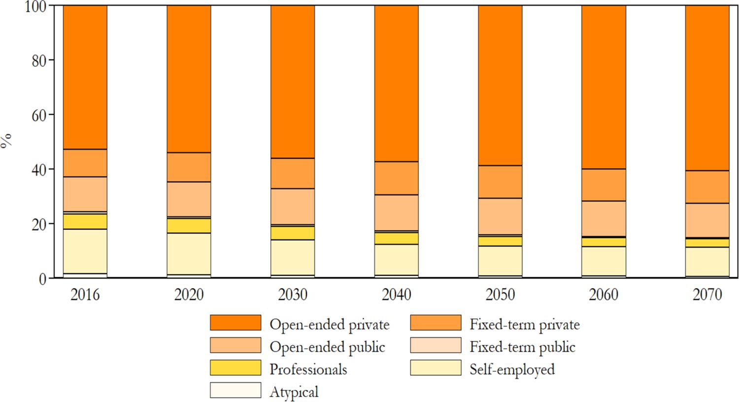
Repartition by work category. Note: Working pensioners are not considered. ISTAT statistics enable the validation of work categories at a more aggregate level compared with T-DYMM’s outputs. We observe that simulation results adhere almost perfectly to reference statistics in the period 2018–2020, while there are no disaggregated statistics for previous years. Further details are available upon request to the authors. Source: Authors’ elaborations of simulation results and ISTAT statistics.
T-DYMM has essentially been employed for adequacy assessments of the Italian pension system; hence, particular attention should be paid to results stemming from the Pension module. Appendix A2 compares model outputs for old-age/seniority, survivor and incapacity pensions with external totals. T-DYMM appears to correctly represent the differences across genders, as survivor pensions are much more common for women. However, despite our work to ensure the representativeness of the sample, it is to be expected that for smaller groups – such as recipients of incapacity pensions – simulations may be less precise. Still, when old-age/senioriy, survivor and incapacity pensioners are considered together, the age distribution for males and females seems aligned to administrative data (see Figure 8). According to our simulations, average retirement ages would increase by about five years for male workers and over six years for their female counterparts over the simulation period (see Figure 9).18 In line with expectations, the average retirement ages for women equal those of their male counterparts in the first few years of the simulation and, as a result of discrepancies within the labour market, later surpass it. For the first years of the simulations, differences between T-DYMM results and reference data can be traced in the limited representativeness in the annual flows of new pensioners (compared to stock figures) and in the fact that T-DYMM does not simulate a number of minor special retirement schemes that generally reduce age requirements for specific categories of workers. The aggregate replacement ratio (ARR) increases by about 10 p.p. in the first decade of the simulation, in line with recent trends,19 then decreases and stabilises at a little over 50% after 2040 (see Figure 9). If we differentiate by gender, the dynamics are opposite in the first 10 years of the simulation: women are still less protected by the pension system than men are, in terms of coverage, but are projected to recover the gap in terms of the ARR by 2030, as a result of growing employment rates in the past few decades.
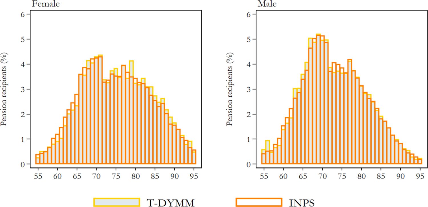
Old-age/seniority, survivor and incapacity pension recipients in 2017 by gender and age. Note: Individuals between ages 55 and 95 are included. The reference distribution is derived from INPS micro data on pensions (the same data employed for AD-SILC but relative to the last year available). Source: Authors’ elaborations of simulation results and INPS micro data.
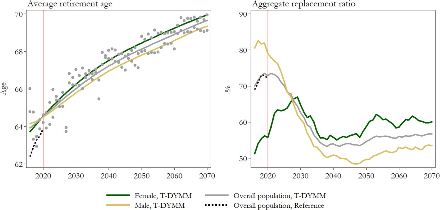
Average retirement age and aggregate replacement ratio by gender. Note: Lowess smoothing for T-DYMM average retirement ages excluding ‘Old age 3’ pensioners. The reference values for the average retirement age derive from the Italian State General Accounting Department (Ragioneria Generale dello Stato, RGS) statistics, while they refer to Eurostat statistics for the aggregate replacement ratio. Source: Authors’ elaborations of simulation results, RGS statistics and Eurostat statistics.
The validation of wealth outcomes encounters a common issue inherent to wealth data - the absence of comprehensive administrative information against which to benchmark simulation results. This contrasts with the situation for household income, which will be discussed later in this section. Nevertheless, a comparison between average wealth figures derived from National Accounts (NA) and T-DYMM for the period 2016-2020 can be provided (see Appendix A2).
Initial values for house wealth averages in T-DYMM, sourced from administrative data, largely align with reference statistics. However, this congruity does not extend to financial wealth and liabilities, which necessitate a complex statistical matching process using SHIW data, post adjustments for under-reporting in both ownership and volumes of financial activities. The discrepancy in net wealth averages between the model and NA diminishes in the period 2016-2020, reflecting a risk for over-accumulation of wealth in the long term. Wealth accumulation channels encompass: i) returns on wealth, ii) savings, and iii) intergenerational transfers, each with potential pitfalls. For i), we aligned to S&P 500 data for the first years of the simulation (2016-2021). That could lead to overly optimistic results, given that S&P 500 comprises a selection of high-quality investments. This optimism might persist post-2021, during which steadily positive returns are assumed. Regarding savings, the model’s exclusion of liabilities for the consumption of basic goods could result in an overestimation of net wealth for some households. Lastly, the closed population approach does not account for potential wealth loss due to unfulfilled wills in the intergenerational transfer channel.
Long-term wealth outcomes are depicted in Figure 10, with a focus on two principal indicators related to wealth distribution and stock accumulation. The Gini index of net wealth, that is equal to 0.60 in 2016, suggests that wealth inequality remains relatively stable for the first 40 years of the simulation before it begins to increase post-2055, reaching a level of 0.67 in 2070. This rise is primarily attributed to intergenerational transfers, particularly inheritances, whose significance in explaining wealth inequality variations amplifies over time. In terms of accumulation, the wealth-to-income ratio (WIR) escalates in the initial simulation years, coinciding with a positive gap between capital returns and wage and pension growth (the average of yearly total returns on stocks for 2016-2021 was 21.6% according to S&P 500). This upward trend ceases post-2021, due to model assumptions that assume a reduction in the discrepancy between capital and labour income growth rates for the period 2022-2070 and the WIR stabilizes around 10 in the long term. The WIR from T-DYMM is compared with that from NA for the period 2016-2020. The initial gap (2016-2017), which subsequently contracts and disappears by 2020, can be traced back to the under-reporting issue at the simulation’s inception and the model’s capacity to address this problem.

Wealth inequality and accumulation. Note: The reference net wealth amount is the sum of the following wealth components: dwellings, currency and deposits, debt securities, shares and other equity, derivatives, mutual fund shares and loans (negative value). See BI and ISTAT (2022) for further details. Gross income is the sum of gross income subject to PIT, self-employment income under substitute tax regimes and rental income that pays the cedolare secca. Source: Authors’ elaborations of simulation results, DF statistics and NA statistics.
The Tax-Benefit module comes at the lowest level of the model hierarchy; hence, it is the one through which we can better evaluate the model’s performance, given that the module’s inputs are the outputs of all previous modules. Moreover, the validation of tax-benefit statistics is facilitated by the extensive availability of aggregate administrative data made publicly available by various institutions. We focus on recipients of income and most sizeable transfers (in terms of aggregate expenditure) instead of monetary amounts because of the greater availability of external data for the former. From this comparison, we observe that the model results adequately fit the reference statistics for the first (2016) and fifth (2020) year of simulation when it comes to gross income recipients (see Figure 11) and PIT taxpayers (see Figure 12). In both cases, the model performs rather poorly at the very end of the left tail of the income distribution, reflecting above all the difficulties we encounter in the exact prediction of labour income components – which form the greatest part of the gross income definition we are referencing – for the most extreme segments of the distribution.
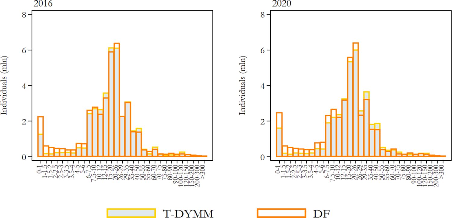
Frequency density function for gross income (values in thousands of euros on the horizontal axis). Note: Gross income is the sum of gross income subject to PIT and rental income subject to the cedolare secca. Source: Authors’ elaborations of simulation results and DF statistics.
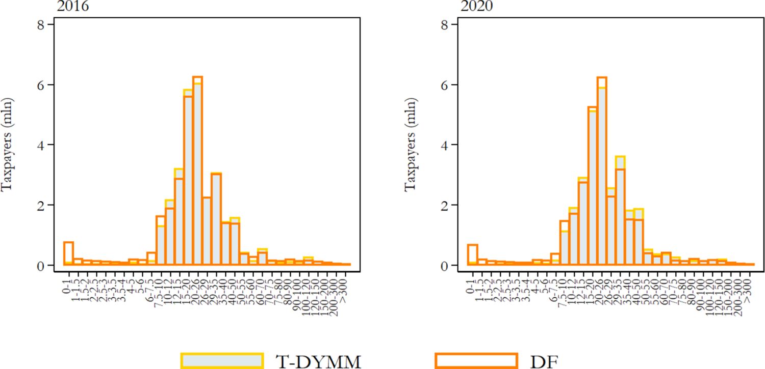
Distribution of PIT taxpayers by gross income group (values in thousands of euros on the horizontal axis). Note: Gross income is the sum of gross income subject to PIT and rental income subject to the cedolare secca. Source: Authors’ elaborations of simulation results and DF statistics.
As for transfers, we note that the model reproduces the age distributions of NASpI recipients and social pension recipients quite accurately (see Appendix A2), and that the goodness of fit increases as the simulation years go by. The model is also able to capture the gender differential in the group of recipients of the integration to old-age/seniority, survivor and incapacity pensions (Integrazione al trattamento minimo), as this measure is more frequent for women.20
The innovations introduced in T-DYMM, specifically the development of the Tax-Benefit module and the Wealth module, make our DMM fit for inequality and poverty analyses. We focus on the medium- and long-term redistributive effect of total transfers and taxes separately, as well as on the projected incidence of poverty. Figure 13 displays trends in income inequality for the overall population and specific age groups, taking the individual as the unit of analysis, while income values are equivalised using the OECD-modified equivalence scale. We discuss the results based on three income aggregates defined as follows: i) gross income before benefits (Y), which includes labour income (net of social security contributions) and productivity bonuses granted to employees, rental income, financial income, retirement income (old-age/seniority, survivor and incapacity pensions, including the integration to these pension benefits), and second- and third-pillar private pensions; ii) gross income after benefits (Y+B), which adds to the previous income definition the full list of in-cash benefits reported in Table 5; iii) disposable income (Y+B-T), which subtracts the personal income tax and proportional taxes listed in Table 4 from gross income after benefits. Given the profound changes in the elderly population due to the rapid increase in retirement ages and employment rates for older workers, in what follows we address this category by analysing the positions of those with ages equal to the standard pensionable age (SPA) and over. We believe that, especially in the long run, a dynamic definition of the elderly better fits our purposes.
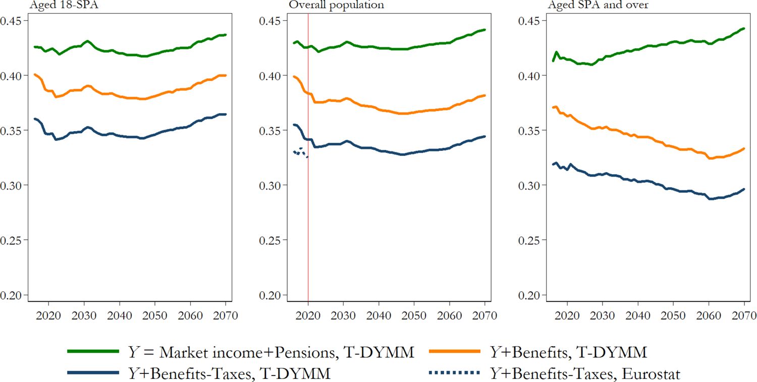
Gini index for equivalised income definitions by age group. Source: Authors’ elaborations of simulation results and Eurostat statistics.
After some disturbance in the first years of the simulation, inequality in gross income before benefits displays an increasing trend, particularly visible for the elderly population. This is due mainly to the increasing share and concentration of capital income.21 Inequalities in gross income after benefits and in disposable income follow a similar trend to that observed for gross income before benefits for the overall and young population. Simulated transfers contribute to a greater extent to the reduction of inequality than taxes in absolute terms.22 This is especially true for the elderly population, for whom the combined effect of ageing and lower pension benefits yields a redistributive effect of transfers three times higher than that of taxes by the end of the simulation. On the transfer side, what drives the greatest reduction in inequality is the role played by the social allowance and disability benefits (both means- and non-means tested measures).23 A large portion of the increase in the social allowance paid out is caused by the fact that NDC pensioners are not entitled to the integration to old-age/seniority, survivor and incapacity pensions, which are included in gross income before benefits and gradually diminish in time.
Figure 14 illustrates the evolution of the incidence of poverty for the overall population and for subgroups by age. For the overall population, we observe that the incidence of poverty slightly decreases over time. The sharp reduction registered in 2022 is due to policy changes to the system of family allowances, i.e. the introduction of the AUU and consequent abrogation of the ANF, the tax credit for dependent children below 21 years old and other bonuses.24 We also observe that working-age individuals are more likely to be poor (in relative terms) than the elderly. The gap between age groups narrows down until 2045 and then slightly increases, but stays lower than its initial level. The upward trend of the poverty incidence curve for the elderly followed by a downward trend from 2045 is attributable to reasons related both to the labour market and pension reforms (Conti et al., 2021). The initial steep increase reflects the discontinuity in careers and stagnation in labour income that have affected Italy in the past 20 years. Pension benefits are also expected to decrease as the transition from the DB system to the less generous NDC rules progresses. By 2045, such transition is accomplished, and the careers of most individuals entering retirement have been lived in simulation (where no negative shock to the economy is assumed). Hence, the incidence in poverty for the elderly decreases slightly in the last decades of the simulation.

At-risk-of-poverty rate by age group. Source: Authors’ elaborations of simulation results and Eurostat statistics.
In Figure 13 and 14, the contained differences between T-DYMM’s results and Eurostat estimates can derive both from the differences in sources for income values (administrative data for T-DYMM, survey data for Eurostat) and from the fact that T-DYMM does not include all existing transfers and sources of income.
5. Conclusions
This paper elucidates the structure and capabilities of T-DYMM, as well as the distinctive and unique features of its underlying dataset, AD-SILC. The latter comprises data from the Italian segment of the European Union Statistics on Income and Living Conditions (IT-SILC) survey, merged with administrative records from various sources and SHIW data. This amalgamation offers a wealth of information on individuals’ socio-economic attributes, their employment histories, disposable income, financial and real wealth. AD-SILC forms the nucleus of the estimation and operational processes of T-DYMM, an encompassing discrete-time dynamic microsimulation model devised for the analysis of the distributional features of the Italian social security system. The model is best suited for simulations over the medium- and long-term horizons and encompasses five modules: demographic, labour market, pension, wealth, and tax-benefit. The recent incorporation of the Wealth module and the expansion of the Tax-Benefit module to cover the vast majority of national-level direct taxes and transfers have extended T-DYMM’s scope of analysis to inequality and poverty. Several areas of potential enhancement and expansion have been identified. The team is presently examining the incorporation of heterogeneity in mortality rates, i.e., distributing average mortality rates (by age and gender) across socio-economic conditions and labour market attributes. A refinement of retirement choices is in progress, with the utility function of potential retirees incorporating a broader set of variables, and risk aversion and leisure preference parameters being estimated based on AD-SILC. T-DYMM could also contribute to under-explored future research directions within the dynamic microsimulation modeling domain, such as the implications of alternative alignment methodologies and the incorporation of behavioural responses in labour supply.
Significant effort has been devoted to validating baseline results by comparing model outputs with external statistics, as far as data availability permits. This methodology, while not yet widely embraced in the development of dynamic models, due to the inherent challenges and to a lack of collective recognition in the microsimulation community, could serve as a reference for defining standard practices for validation. We followed the recent input on the topic by Liégeois et al. (2021) in this respect. We posit that the comprehensive analysis presented herein enhances the model’s credibility and transparency. It also provides a foundation for future studies aiming to conduct scenario analyses using the model.
Footnotes
1.
A closed model allows individuals to only form couples with other individuals within the sample. On the contrary, open models artificially create spouses of sample individuals who experience the marriage event. In both cases, newborns and migrants are generated by a cloning routine.
2.
We observe that reported earnings in INPS archives are in line with declared earnings from tax records, except for specific categories of self-employed individuals – i.e. individuals with declared earnings below the minimum statutory thresholds set for the payment of social insurance contributions (SICs). In the Italian tax system, self-employed workers are required to pay a fixed amount of SICs regardless of the amount of earnings declared for tax purposes. This means that, for a series of observations in the AD-SILC dataset, the reported income for SIC-related purposes is systematically greater than the declared income for tax purposes. The use of earnings from the INPS archives for the estimate of self-employed workers’ labour income would lead to an underestimation of poverty among these workers and would likely inflate poverty thresholds calculated for the overall population. To tackle this issue, we have imputed via statistical matching the ratio between earnings declared for tax purposes and those collected in the INPS archives for self-employed workers, with reported earnings for SIC-related purposes exactly equal to the observed statutory thresholds in the AD-SILC dataset. Estimating tax evasion is outside of the scope of this intervention.
3.
We perform a procedure to correct the initial values of financial wealth and liabilities in order to reduce the relevance of under-reporting (Bonci et al., 2005). The correction procedure follows the three steps laid out in Boscolo (2019): i) correction for ownership of financial instruments, following Brandolini et al. (2009); ii) attribution of financial wealth amounts to households of ‘new’ owners; and iii) correction for the amount of financial wealth owned, following D’Aurizio et al. (2006). The total amount of financial wealth for adjusted SHIW data amounts to 2,547 billion euros. The implemented procedure significantly reduces the gap between SHIW totals and National Accounts (NA) totals, as the adjusted total of financial wealth accounts for 78% of the NA, while the original SHIW total accounts for 22%.
4.
As a result, the age of the sample units is scaled back to the year before the interview, leading to the exclusion of individuals born in 2016.
5.
For instance, the ‘consumption/saving’ process, which logically belongs to the Wealth module, is solved last, as one can only compute consumption on the basis of a final definition of income (comprehensive of benefits and net of taxes).
6.
Lack of data on the emigration phenomenon does not allow us to follow individuals who exit the resident sample, hence we do not simulate return migration. We do assume that a portion of immigrants each year was born in Italy, but they are newly formed units that have no history within the model.
7.
For immigrants, education achievements are attributed according to OECD data by gender and area of origin and a limited portion holds elementary education as highest level.
8.
Most models are estimated through pooled OLS estimators, even if AD-SILC has a panel structure. In such data, coefficients encompass two sources of variation: within-subject variability and between-subject variability. Pooled OLS estimators simply treat within- and between-group variation as the same (i.e. they pool data across waves). This choice is pursued either because we tested that the fraction of variance due to individual effects is close to nil or in order to guarantee a coherent amount of individual heterogeneity both in the regressions and in the model (Shmueli, 2010; Martini and Trivellato, 1997). For months and wages, instead, we use random-effects models, as in this case individual heterogeneity is relevant and can play a role within the microsimulation model. In particular, we use the predicted values of the random effects for in-sample individuals, while for new-born or out-of-sample individuals we impute these values drawing from a normal distribution with the estimated mean and standard deviation. Whenever the sample size is large enough, men and women working trajectories follow separate models, since the literature suggests very different employment dynamics by gender (Bertrand, 2020).
9.
The classification proposed here may differ from the taxonomy reported in the legislation. For instance, the ‘Old Age 1’ criterion is generally referred to as a form of ‘early retirement’, hence viewed in the same category as the ‘Seniority’ criterion. However, because it includes age and amount requirements, we have opted to consider it as a form of old-age retirement.
10.
Decree Law 4/2019 suspended indexation of requirements to life expectancy variations for ‘Seniority’ and ‘Seniority - young workers’ criteria until 2026.
11.
According to the Parliamentary Budget Office (Ufficio Parlamentare di Bilancio, UPB) and INPS in UPB and INPS (2022), in the 2019-2021 period 56% of the women who met requirements and 58% of the men accessed retirement through the ’Quota 100’ channel. T-DYMM results using the choice function are respectively 64% and 62%.
12.
The TFR is a sort of mandatory severance payment for public and private employees. It acts as a deferred share of wage: TFR contributions are withheld and managed by the employer (the accrual rate is mandated by law and equal to 1.5% plus 75% of inflation growth), who has to pay the accumulated amount to the employee in the event of dismissal or retirement (the TFR may also be anticipated in part under a very limited set of circumstances, T-DYMM only considers the possibility of withdrawing up to 70% of the TFR in order to buy a first house). A crucial change in the legislation concerning TFR took place in 2007, when the so-called ‘silent consent’ formula was introduced: if workers do not explicitly disagree, their TFR flows (not the stock already accrued by firms) are transferred from firms to the selected pension fund. According to the latest available data from COVIP (2018), only about 23% of the overall amount of accrued TFR has been transferred to pension funds.
13.
Following the same reasoning adopted for the Labour Market module, we select explanatory variables for which we can project the evolution over the simulation period.
14.
As for deductions, we refer to social insurance contributions paid by self-employed workers, the cadastral value of the main residence and contributions to private pension plans; regarding tax credits, the most relevant ones are the tax credit for labour and retirement income and tax credits for dependent family members.
15.
Among residual tax expenditures, we do not include the tax credit introduced in 2020 for the implementation of energy-efficiency refurbishments and consolidation measures against the seismic risk of buildings (Superbonus 110%) due to a lack of data.
16.
The ‘unemployment state’ (stato di disoccupazione), the state of individuals who are not in work but are looking for and are available to work, is a necessary condition to access unemployment benefits under the current legislation.
17.
The number of self-employed workers decreased by about 20% from 1990 to 2019 (ISTAT, 2019).
18.
‘Old age 3’ pensioners are excluded from these statistics in order to facilitate a comparison between results at the beginning and the end of the simulations. The ‘Old age 3’ criterion allows retirement to individuals that would have simply lost their contributions under the previous legislation but pays out very low pensions as a result of the few years spent in the workforce. Furthermore, upon reaching the ‘Old age 2’ age requirement, poor elderly people can always access a social allowance, the assegno sociale.
19.
The 2021 Adequacy Report from the European Commission (European Commission DG EMPL, 2021) registers a 22 p.p. variation of the indicator in the 2008–2019 period.
20.
The number of female (male) recipients in 2019 amounts to 2.0 (0.4) millions according to model outputs, while INPS statistics report a number of female (male) recipients of 2.3 (0.5) millions.
21.
Capital income, which is the sum of financial income and rental income, accounts for 8.0% of gross income before benefits in 2016 and steadily increases to 16.2% by 2070. The concentration index of capital income with respect to gross income before benefits increases from 0.64 in 2016 to 0.70 by the end of the simulation.
22.
The redistributive effect of transfers (taxes) equals the difference between the Gini index of gross income before benefits (gross income after benefits) and the Gini index of gross income after benefits (disposable income). For the overall population, the redistributive effect of transfers was equal to 0.031 (0.060) in 2016 (2070), while taxes reduced inequality in gross income after benefits by 0.044 (0.037) in 2016 (2070).
23.
The share of recipients amounts respectively to 3.7% (21.0%) and 14.1% (20.3%) of the elderly population in 2016 (2070). Furthermore, disability allowances are more equally distributed by the end of the simulation. The concentration index of the social allowance (disability benefits) with respect to gross income before benefits varies from -0.37 (-0.03) in 2016 to -0.36 (-0.12) in 2070. Note that these statistics are computed using non-equivalised values.
24.
Following the introduction of AUU, we estimate a fall in child poverty from 27.5% in 2021 to 24.6% in 2022.
Appendix A1
T-DYMM’s base year validation
In what follows, we compare distributions of T-DYMM’s base year sample with totals derived from IT-SILC weights and with external totals. First, it should be noted that representativeness is overall preserved when looking at the same dimensions for which the IT-SILC weights have been originally calibrated (see Figure A1.1). Second, the calibration and sampling procedure proves to be effective in overcoming the under- and overestimation of single ages that would emerge if we were to use IT-SILC weights (see Figure A1.2). Furthermore, we observe marginal improvements for many income groups in which the distribution of individuals with gross income subject to PIT is divided (see Figure A1.3). The calibrated distribution adheres almost perfectly to external totals. Table A1.1 gathers the results for selected calibrated characteristics and household distributions. From the comparison we conclude that the representativeness of the sample is systematically improved with regards to the many dimensions we calibrate for. As for household-level characteristics not directly included in the calibration algorithm, we see that the implemented procedure preserves rather accurately the representativeness of two key dimensions: the distribution of households at the regional level and the distribution of households by type (e.g. single, single with children, couple, and so on).
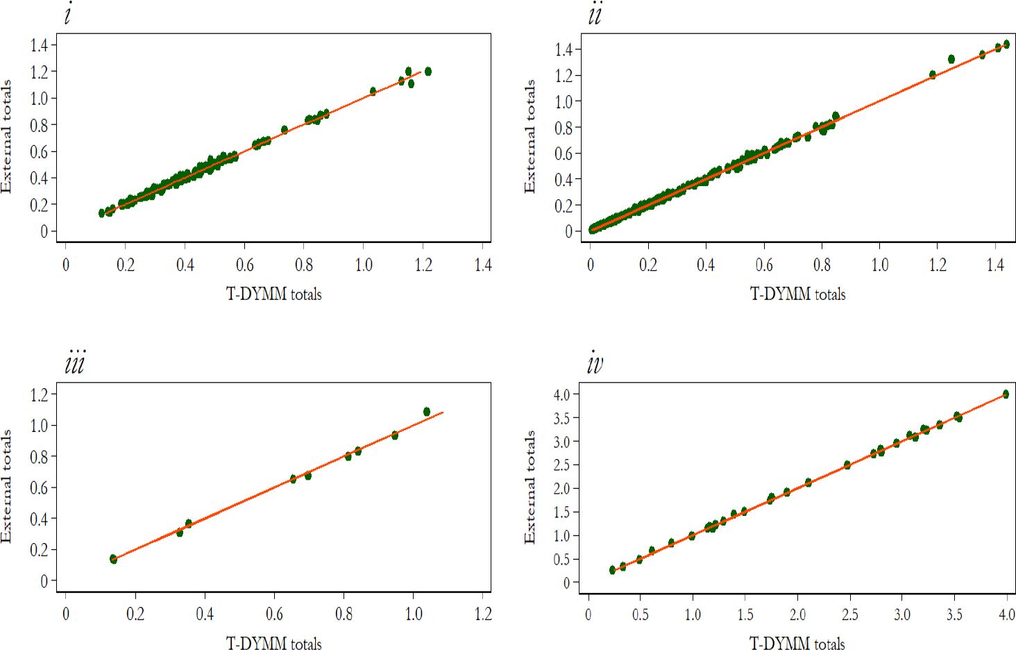
Distributions employed in the calibration of IT-SILC weights (individuals in millions on the horizontal axis). Note: i) distribution of the population at the macro-regional level by gender and fourteen age groups; ii) distribution of the population at the regional level by gender and five age groups; iii) distribution of the foreign population at the macro-regional level by gender; iv) distribution of the population at the macro-regional level by demographic size of the municipality of residence. Source: Authors’ elaborations of AD-SILC 2015 and ISTAT statistics.

Distribution of the population by gender and one-year age group (individuals in millions on the horizontal axis). Source: Authors’ elaborations of AD-SILC 2015 and ISTAT statistics.
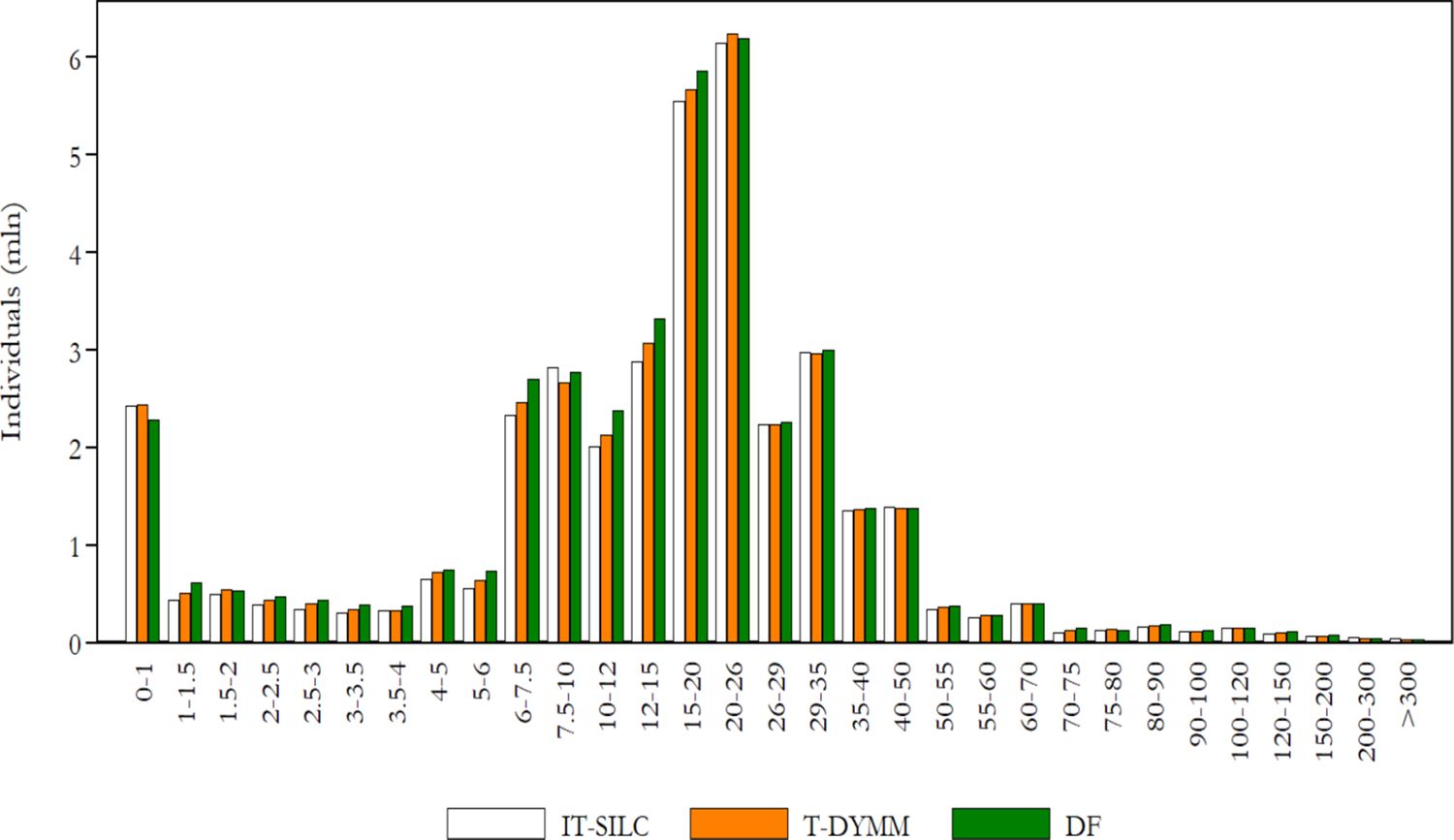
Frequency density function for gross income (values in thousands of euros on the horizontal axis). Note: Gross income is the sum of gross income subject to PIT and rental income subject to the cedolare secca. Source: Authors’ elaborations of AD-SILC 2015 and DF statistics.
Comparison between sample totals and external totals for selected distributions.
| Variable | (1) IT-SILC totals | (2) T-DYMM totals | (3) External totals | (1)/(3) | (2)/(3) |
|---|---|---|---|---|---|
| Individuals | 60,323,126 | 60,631,408 | 60,665,551 | 0.994 | 0.999 |
| Households (in thousands) | 25,821 | 25,429 | 25,386 | 1.017 | 1.002 |
| Ratio individuals/households | 2.336 | 2.384 | 2.390 | 0.977 | 0.998 |
| Foreign population by gender, area of birth and educational attainment: | |||||
| Female – EU – Upper secondary | 566,866 | 540,119 | 532,951 | 1.064 | 1.013 |
| Female – EU – Tertiary | 140,621 | 186,397 | 194,004 | 0.725 | 0.961 |
| Female – non-EU – Upper secondary | 689,547 | 706,173 | 695,296 | 0.992 | 1.016 |
| Female – non-EU – Tertiary | 311,078 | 307,186 | 302,485 | 1.028 | 1.016 |
| Male – EU – Upper secondary | 287,465 | 334,650 | 345,220 | 0.833 | 0.969 |
| Male – EU – Tertiary | 93,373 | 61,285 | 63,090 | 1.480 | 0.971 |
| Male – non-EU – Upper secondary | 609,550 | 572,669 | 573,095 | 1.064 | 0.999 |
| Male – non-EU – Tertiary | 151,188 | 205,723 | 206,235 | 0.733 | 0.998 |
| Population by number of household members (in thousands): | |||||
| 1 | 8,369 | 8,032 | 8,016 | 1.044 | 1.002 |
| 2 | 14,332 | 13,866 | 13,838 | 1.036 | 1.002 |
| 3 | 15,141 | 15,043 | 15,111 | 1.002 | 0.995 |
| 4 | 16,112 | 16,075 | 16,200 | 0.995 | 0.992 |
| 5 | 4,890 | 5,400 | 5,290 | 0.924 | 1.021 |
| 6 or more | 1,478 | 2,214 | 2,211 | 0.668 | 1.001 |
| Individuals with retirement income at the macro-regional level by gender: | |||||
| North West – Female | 2,218,088 | 2,367,979 | 2,378,635 | 0.933 | 0.996 |
| North East – Female | 1,546,322 | 1,675,793 | 1,675,812 | 0.923 | 1 |
| Middle – Female | 1,599,179 | 1,667,401 | 1,671,085 | 0.957 | 0.998 |
| South – Female | 1,701,624 | 1,753,352 | 1,766,032 | 0.964 | 0.993 |
| Islands – Female | 834,713 | 835,608 | 832,585 | 1.003 | 1.004 |
| North West – Male | 1,993,336 | 2,033,838 | 2,059,497 | 0.968 | 0.988 |
| North East – Male | 1,473,823 | 1,498,042 | 1,479,615 | 0.996 | 1.012 |
| Middle – Male | 1,443,607 | 1,485,073 | 1,486,315 | 0.971 | 0.999 |
| South – Male | 1,608,304 | 1,593,656 | 1,616,762 | 0.995 | 0.986 |
| Islands – Male | 796,957 | 787,546 | 795,288 | 1.002 | 0.990 |
| Individuals with retirement income by gender and six age groups: | |||||
| Female – 0-54 | 564,506 | 600,895 | 604,675 | 0.934 | 0.994 |
| Female – 55-64 | 1,023,141 | 1,067,015 | 1,072,665 | 0.954 | 0.995 |
| Female – 65-69 | 1,443,927 | 1,487,870 | 1,488,105 | 0.970 | 1 |
| Female – 70-74 | 1,208,479 | 1,276,298 | 1,269,707 | 0.952 | 1.005 |
| Female – 75-79 | 1,264,050 | 1,348,517 | 1,364,252 | 0.927 | 0.988 |
| Female – 80 and over | 2,395,823 | 2,519,538 | 2,524,745 | 0.949 | 0.998 |
| Male – 0-54 | 741,462 | 694,984 | 711,781 | 1.042 | 0.976 |
| Male – 0-54 | 741,462 | 694,984 | 711,781 | 1.042 | 0.976 |
| Male – 65-69 | 1,606,143 | 1,605,099 | 1,607,490 | 0.999 | 0.999 |
| Male – 70-74 | 1,262,353 | 1,271,212 | 1,301,312 | 0.970 | 0.977 |
| Male – 75-79 | 1,175,818 | 1,227,220 | 1,218,628 | 0.965 | 1.007 |
| Male – 80 and over | 1,392,296 | 1,469,307 | 1,472,586 | 0.945 | 0.998 |
| Individuals with retirement income by gender and type of pension: | |||||
| Female – Old-age and seniority pensions | 4,709,966 | 5,204,113 | 5,196,325 | 0.906 | 1.001 |
| Female – Inability pensions | 565,080 | 617,424 | 624,406 | 0.905 | 0.989 |
| Female – Survivors’ pensions | 3,605,291 | 4,034,618 | 4,032,187 | 0.894 | 1.001 |
| Female – Disability pensions | 1,416,051 | 1,813,111 | 1,824,118 | 0.776 | 0.994 |
| Female – Social pension | 518,856 | 536,305 | 541,679 | 0.958 | 0.990 |
| Male – Old-age and seniority pensions | 5,716,676 | 6,319,952 | 6,377,756 | 0.896 | 0.991 |
| Male – Inability pensions | 606,074 | 642,345 | 652,098 | 0.929 | 0.985 |
| Male – Survivors’ pensions | 583,017 | 603,947 | 617,234 | 0.945 | 0.978 |
| Male – Disability pensions | 992,888 | 1,201,027 | 1,219,673 | 0.814 | 0.985 |
| Male – Social pension | 266,998 | 297,015 | 304,413 | 0.877 | 0.976 |
| Retired workers by gender (in thousands): | |||||
| Female | 196 | 115 | 111 | 1.766 | 1.036 |
| Male | 536 | 321 | 331 | 1.619 | 0.970 |
| In-work individuals by area of birth (in thousands): | |||||
| Italy | 20,107 | 20,132 | 20,106 | 1 | 1.001 |
| EU or non-EU | 3,033 | 2,326 | 2,359 | 1.286 | 0.986 |
| In-work individuals by employment status (in thousands): | |||||
| Employees | 18,042 | 17,008 | 16,988 | 1.062 | 1.001 |
| Freelancers | 1,161 | 1,314 | 1,327 | 0.875 | 0.990 |
| Craftsmen, traders and farmers | 3,387 | 3,793 | 3,801 | 0.891 | 0.998 |
| Atypical workers (co.co.co.) | 550 | 344 | 349 | 1.576 | 0.986 |
| Employees by type of contract (in thousands): | |||||
| Open-ended | 15,290 | 14,615 | 14,605 | 1.047 | 1.001 |
| Fixed-term | 2,752 | 2,393 | 2,383 | 1.155 | 1.004 |
| Full-time | 14,324 | 13,634 | 13,642 | 1.050 | 0.999 |
| Part-time | 3,718 | 3,373 | 3,346 | 1.111 | 1.008 |
| Population by gender and civil status: | |||||
| Female – Single | 11,444,708 | 11,878,040 | 11,900,653 | 0.962 | 0.998 |
| Female – Married or separated | 14,719,913 | 14,669,927 | 14,683,481 | 1.002 | 0.999 |
| Female – Divorced | 824,754 | 862,563 | 871,345 | 0.947 | 0.990 |
| Female – Widow | 4,022,839 | 3,753,115 | 3,753,751 | 1.072 | 1 |
| Male – Single | 13,305,714 | 13,646,650 | 13,641,747 | 0.975 | 1 |
| Male – Married or separated | 14,586,291 | 14,448,378 | 14,485,092 | 1.007 | 1 |
| Male – Divorced | 477,936 | 579,280 | 584,343 | 0.818 | 0.991 |
| Households at the regional level (in thousands): | |||||
| Male – Widower | 940,970 | 752,454 | 745,139 | 1.263 | 1.010 |
| Piemonte | 2,008 | 1,963 | 1,950 | 1.030 | 1.007 |
| Valle d’Aosta | 61 | 125 | 62 | 0.984 | 2.016 |
| Liguria | 771 | 788 | 756 | 1.020 | 1.042 |
| Lombardia | 4,418 | 4,299 | 4,222 | 1.046 | 1.018 |
| Bolzano | 217 | 246 | 215 | 1.009 | 1.144 |
| Trento | 233 | 254 | 228 | 1.022 | 1.114 |
| Veneto | 2,059 | 2,022 | 1,983 | 1.038 | 1.020 |
| Friuli-Venezia Giulia | 559 | 622 | 544 | 1.028 | 1.143 |
| Emilia-Romagna | 1,993 | 1,928 | 1,961 | 1.016 | 0.983 |
| Toscana | 1,643 | 1,614 | 1,636 | 1.004 | 0.987 |
| Umbria | 383 | 420 | 379 | 1.011 | 1.108 |
| Marche | 644 | 683 | 641 | 1.005 | 1.066 |
| Lazio | 2,631 | 2,528 | 2,601 | 1.012 | 0.972 |
| Abruzzo | 555 | 532 | 549 | 1.011 | 0.969 |
| Molise | 131 | 167 | 131 | 1 | 1.275 |
| Campania | 2,157 | 2,068 | 2,173 | 0.993 | 0.952 |
| Puglia | 1,587 | 1,549 | 1,593 | 0.996 | 0.972 |
| Basilicata | 231 | 248 | 238 | 0.971 | 1.042 |
| Calabria | 800 | 740 | 806 | 0.993 | 0.918 |
| Sicilia | 2,022 | 1,930 | 2,022 | 1 | 0.955 |
| Sardegna | 719 | 699 | 696 | 1.033 | 1.004 |
| Households by type (in thousands): | |||||
| Single | 8,369 | 8,175 | 8,312 | 1.007 | 0.984 |
| Single with children | 2,216 | 2,083 | 2,360 | 0.939 | 0.883 |
| Couple | 5,142 | 4,973 | 5,110 | 1.006 | 0.973 |
| Couple with children | 8,692 | 8,701 | 8,754 | 0.993 | 0.994 |
| Other | 1,403 | 1,494 | 850 | 1.651 | 1.758 |
-
Source: Authors’ elaborations of AD-SILC 2015 and statistics from different institutes (Eurostat, ISTAT, INPS and DF).
Appendix A2
Validation of T-DYMM’s baseline results, 2016–2020
| Variable | (1) T-DYMM totals | (2) External totals | (1)/(2) | ||||||||||||
|---|---|---|---|---|---|---|---|---|---|---|---|---|---|---|---|
| 2016 | 2017 | 2018 | 2019 | 2020 | 2016 | 2017 | 2018 | 2019 | 2020 | 2016 | 2017 | 2018 | 2019 | 2020 | |
| Share of households by number of members (%):a | |||||||||||||||
| 1 | 32.4 | 33.9 | 35.3 | 36.4 | 37.4 | 31.6 | 31.9 | 33.0 | 33.3 | 32.9 | 1.025 | 1.063 | 1.068 | 1.092 | 1.137 |
| 2 | 27.3 | 27.3 | 27.4 | 27.4 | 27.3 | 27.3 | 27.5 | 27.1 | 27.1 | 27.7 | 1 | 0.994 | 1.010 | 1.011 | 0.987 |
| 3 | 19.1 | 17.9 | 17.1 | 16.4 | 15.9 | 19.8 | 19.6 | 19.5 | 19.3 | 19.0 | 0.963 | 0.916 | 0.876 | 0.849 | 0.836 |
| 4 | 15.6 | 14.9 | 14.3 | 13.8 | 13.2 | 16.0 | 15.7 | 15.1 | 15.1 | 15.3 | 0.972 | 0.952 | 0.949 | 0.912 | 0.865 |
| 5 | 4.3 | 4.4 | 4.5 | 4.5 | 4.5 | 4.2 | 4.1 | 4.0 | 4.0 | 3.9 | 1.024 | 1.073 | 1.117 | 1.130 | 1.158 |
| 6 or more | 1.4 | 1.5 | 1.5 | 1.6 | 1.6 | 1.2 | 1.2 | 1.2 | 1.3 | 1.3 | 1.169 | 1.212 | 1.251 | 1.194 | 1.248 |
| Average hourly salary for private sector employees by (in euros): | |||||||||||||||
| i) Contract duration: | |||||||||||||||
| Open-ended | 14.3 | 14.3 | 14.6 | 14.9 | 15.4 | 14.8 | 15.1 | 15.1 | 15.2 | 15.5 | 0.969 | 0.949 | 0.968 | 0.980 | 0.994 |
| Fixed-term | 10.7 | 10.8 | 11.1 | 11.4 | 11.8 | 12.1 | 12.1 | 12.1 | 12.1 | 12.1 | 0.886 | 0.893 | 0.920 | 0.939 | 0.975 |
| ii) Educational attainment: | |||||||||||||||
| Up to lower secondary | 11.7 | 11.8 | 12.0 | 12.2 | 12.7 | 12.0 | 12.1 | 12.1 | 12.2 | 12.4 | 0.973 | 0.974 | 0.996 | 1.002 | 1.025 |
| Upper secondary | 13.9 | 14.0 | 14.3 | 14.5 | 15.0 | 14.3 | 14.3 | 14.2 | 14.4 | 14.6 | 0.975 | 0.978 | 1.004 | 1.009 | 1.030 |
| Tertiary | 17.5 | 17.4 | 17.6 | 17.9 | 18.2 | 19.1 | 19.2 | 19.2 | 19.5 | 19.9 | 0.915 | 0.907 | 0.919 | 0.920 | 0.916 |
| iii) Area of birth: | |||||||||||||||
| Abroad | 10.0 | 10.0 | 10.3 | 10.5 | 10.9 | 11.7 | 11.8 | 11.8 | 11.9 | 12.2 | 0.852 | 0.846 | 0.876 | 0.886 | 0.896 |
| Italy | 14.4 | 14.5 | 14.8 | 15.1 | 15.6 | 14.4 | 14.5 | 14.4 | 14.6 | 14.9 | 0.999 | 1.001 | 1.025 | 1.032 | 1.046 |
| iv) Age group: | |||||||||||||||
| 15-29 | 10.4 | 10.4 | 10.5 | 10.6 | 10.9 | 11.2 | 11.4 | 11.3 | 11.4 | 11.5 | 0.932 | 0.915 | 0.926 | 0.929 | 0.945 |
| 30-49 | 14.0 | 14.0 | 14.1 | 14.4 | 14.8 | 14.0 | 14.1 | 14.1 | 14.3 | 14.5 | 0.998 | 0.993 | 1.003 | 1.009 | 1.022 |
| 50 or more | 15.1 | 15.4 | 16.0 | 16.2 | 16.7 | 16.3 | 16.4 | 16.2 | 16.3 | 16.6 | 0.925 | 0.941 | 0.987 | 0.993 | 1.005 |
| v) Gender: | |||||||||||||||
| Female | 13.1 | 13.2 | 13.5 | 13.8 | 14.2 | 13.0 | 13.1 | 13.0 | 13.2 | 13.6 | 1.009 | 1.006 | 1.035 | 1.045 | 1.047 |
| Male | 14.1 | 14.2 | 14.5 | 14.7 | 15.2 | 14.7 | 14.7 | 14.6 | 14.8 | 15.1 | 0.962 | 0.967 | 0.990 | 0.992 | 1.009 |
| Number of pensions by gender and typology (in thousands):b | |||||||||||||||
| Female – Old-age/seniority | – | 4,993 | 4,887 | 4,918 | 4,874 | – | 5,189 | 5,155 | 5,128 | 5,146 | – | 0.962 | 0.946 | 0.959 | 0.947 |
| Male – Old-age/seniority | – | 6,105 | 6,012 | 6,177 | 6,086 | – | 6,155 | 6,166 | 6,200 | 6,303 | – | 0.922 | 0.975 | 0.996 | 0.966 |
| Female – Survivor | – | 3,840 | 3,804 | 3,774 | 3,744 | – | 3,838 | 3,806 | 3,773 | 3,760 | – | 1.001 | 0.999 | 1 | 0.996 |
| Male – Survivor | – | 558 | 561 | 571 | 577 | – | 540 | 542 | 545 | 550 | – | 1.033 | 1.035 | 1.048 | 1.049 |
| Female – Incapacity | – | 516 | 495 | 473 | 454 | – | 599 | 558 | 524 | 494 | – | 0.861 | 0.887 | 0.903 | 0.919 |
| Male – Incapacity | – | 586 | 574 | 555 | 545 | – | 637 | 616 | 612 | 600 | – | 0.920 | 0.932 | 0.907 | 0.908 |
| Average monthly pension by gender and typology (in euros):b | |||||||||||||||
| Female – Old-age/seniority | – | 877 | 909 | 957 | 993 | – | 960 | 989 | 1025 | 1057 | – | 0.914 | 0.919 | 0.933 | 0.940 |
| Male – Old-age/seniority | – | 1,748 | 1,781 | 1,819 | 1,842 | – | 1,583 | 1,616 | 1,653 | 1,683 | – | 1.104 | 1.102 | 1.101 | 1.094 |
| Female – Survivor | – | 727 | 744 | 759 | 772 | – | 711 | 724 | 737 | 746 | – | 1.023 | 1.028 | 1.030 | 1.035 |
| Male – Survivor | – | 439 | 446 | 453 | 452 | – | 466 | 474 | 481 | 486 | – | 0.941 | 0.941 | 0.943 | 0.931 |
| Female – Incapacity | – | 702 | 718 | 726 | 726 | – | 690 | 708 | 728 | 746 | – | 1.017 | 1.013 | 0.997 | 0.974 |
| Male – Incapacity | – | 913 | 915 | 895 | 891 | – | 1,076 | 1,100 | 1,116 | 1,132 | – | 0.849 | 0.831 | 0.802 | 0.787 |
| Average age of pensioners by gender and typology:b | |||||||||||||||
| Female – Old-age/seniority | – | 75.7 | 76.2 | 76.2 | 76.4 | – | 75.4 | 75.7 | 76.1 | 76.4 | – | 1.005 | 1.006 | 1.002 | 1.001 |
| Male – Old-age/seniority | – | 73.5 | 73.9 | 73.9 | 74.1 | – | 74.2 | 74.5 | 74.7 | 74.9 | – | 0.990 | 0.992 | 0.989 | 0.989 |
| Female – Survivor | – | 77.8 | 78.0 | 78.1 | 78.1 | – | 78.6 | 78.7 | 78.9 | 79.1 | – | 0.990 | 0.991 | 0.990 | 0.988 |
| Male – Survivor | – | 75.5 | 75.8 | 76.2 | 76.4 | – | 75.4 | 75.5 | 75.6 | 75.8 | – | 1.002 | 1.004 | 1.007 | 1.008 |
| Female – Incapacity | – | 72.5 | 72.3 | 72.3 | 71.9 | – | 77.5 | 77.0 | 76.4 | 75.8 | – | 0.936 | 0.939 | 0.946 | 0.949 |
| Male – Incapacity | – | 66.7 | 66.7 | 66.5 | 66.0 | – | 68.8 | 68.4 | 68.0 | 67.7 | – | 0.969 | 0.976 | 0.978 | 0.975 |
| Average wealth values (in thousands of euros):c | |||||||||||||||
| Net wealth | 277.8 | 283.1 | 287.2 | 293.8 | 299.8 | 306.6 | 309.0 | 298.2 | 304.8 | 308.1 | 0.906 | 0.916 | 0.963 | 0.964 | 0.973 |
| House wealth | 195.1 | 196.3 | 197.9 | 198.5 | 198.5 | 205.7 | 203.8 | 201.4 | 201.3 | 201.8 | 0.948 | 0.963 | 0.982 | 0.986 | 0.984 |
| Financial wealth | 93.8 | 99.5 | 103.7 | 111.3 | 118.6 | 128.4 | 133.0 | 124.9 | 132.2 | 135.5 | 0.730 | 0.748 | 0.831 | 0.842 | 0.875 |
| Liabilities | 11.1 | 12.7 | 14.3 | 16.0 | 17.4 | 27.5 | 27.8 | 28.1 | 28.7 | 29.1 | 0.405 | 0.457 | 0.511 | 0.557 | 0.596 |
| Share of NASpI recipients by age group (%):d | |||||||||||||||
| 24 or less | 11.2 | 9.1 | – | – | – | 9.1 | 9.4 | – | – | – | 1.231 | 0.968 | – | – | – |
| 25-29 | 16.2 | 13.9 | – | – | – | 13.5 | 13.3 | – | – | – | 1.200 | 1.045 | – | – | – |
| 30-34 | 17.3 | 13.5 | – | – | – | 14.1 | 13.7 | – | – | – | 1.227 | 0.985 | – | – | – |
| 35-39 | 12.6 | 14.2 | – | – | – | 14.1 | 13.6 | – | – | – | 0.894 | 1.044 | – | – | – |
| 40-44 | 10.9 | 13.1 | – | – | – | 13.9 | 13.6 | – | – | – | 0.784 | 0.963 | – | – | – |
| 45-49 | 12.3 | 10.9 | – | – | – | 12.6 | 12.5 | – | – | – | 0.976 | 0.872 | – | – | – |
| 50-54 | 7.3 | 11.1 | – | – | – | 10.5 | 10.8 | – | – | – | 0.695 | 1.028 | – | – | – |
| 55 or more | 12.3 | 14.2 | – | – | – | 12.2 | 13.1 | – | – | – | 1.008 | 1.084 | – | – | – |
| Share of social pension recipients by age group (%): | |||||||||||||||
| 65-69 | 25.9 | 24.5 | 20.1 | 20.4 | 19.8 | 34.1 | 33.3 | 27.5 | 22.1 | 21.6 | 0.760 | 0.736 | 0.731 | 0.923 | 0.917 |
| 70-74 | 25.3 | 25.3 | 26.1 | 27.0 | 30.4 | 26.5 | 27.3 | 30.3 | 33.1 | 33.7 | 0.955 | 0.927 | 0.861 | 0.816 | 0.902 |
| 75-79 | 20.6 | 23.4 | 24.4 | 21.1 | 17.6 | 19.5 | 19.3 | 20.5 | 21.4 | 21.0 | 1.056 | 1.212 | 1.190 | 0.986 | 0.838 |
| 80-84 | 16.7 | 15.2 | 16.4 | 20.1 | 20.0 | 11.8 | 11.8 | 12.8 | 13.9 | 14.1 | 1.415 | 1.288 | 1.281 | 1.446 | 1.418 |
| 85-89 | 9.8 | 8.1 | 9.3 | 7.5 | 8.0 | 5.9 | 5.9 | 6.3 | 6.7 | 6.7 | 1.661 | 1.373 | 1.476 | 1.119 | 1.194 |
| 90-94 | 1.1 | 2.7 | 3.0 | 3.1 | 3.6 | 1.9 | 2.0 | 2.1 | 2.3 | 2.4 | 0.579 | 1.350 | 1.429 | 1.348 | 1.500 |
| 95 or more | 0.7 | 0.9 | 0.6 | 0.8 | 0.6 | 0.4 | 0.5 | 0.5 | 0.6 | 0.6 | 1.750 | 1.800 | 1.200 | 1.333 | 1.000 |
-
Note: External statistics refer to:i) ISTAT for the share of households by number of members and the average monthly salary for private sector employees by socio-demographic characteristics; ii) NA for wealth amounts; and iii) INPS for the remaining statistics. a) In accordance with ISTAT, figures for period t are computed as average of t and t-1. b) Figures before 2017 are not publicly available for public sector workers from INPS. c) The reference net wealth amount is the sum of the following wealth components: dwellings; currency and deposits, debt security, shares and other equity, derivatives, and mutual fund shares for financial wealth; loans as liabilities. d) No external statistics are available in the interval 2018–2020. Source: Authors’ elaborations of simulation results and external statistics.
Appendix A3
Labour Market module regression estimates
Probability of being employed.
| Male | Female | |||
|---|---|---|---|---|
| b | se | b | se | |
| extra-EU born | 0.318*** | (0.042) | 0.250*** | (0.038) |
| studying | -1.022*** | (0.033) | -1.029*** | (0.033) |
| retired | -1.327*** | (0.049) | -1.209*** | (0.069) |
| age | 0.383*** | (0.012) | 0.064*** | (0.005) |
| age2 | -0.010*** | (0.000) | -0.001*** | (0.000) |
| age3 | 0.000*** | (0.000) | ||
| upper sec. degree | 0.250*** | (0.020) | 0.385*** | (0.021) |
| tertiary degree | 0.578*** | (0.032) | 0.850*** | (0.031) |
| disabled | -0.335*** | (0.050) | -0.306*** | (0.058) |
| disability pension | -1.048*** | (0.100) | -1.030*** | (0.096) |
| disability allowance | -1.021*** | (0.125) | -0.864*** | (0.131) |
| incapacity pension | -1.018*** | (0.086) | -1.285*** | (0.138) |
| in couple | 0.107*** | (0.027) | -0.318*** | (0.033) |
| partner working (lag) | 0.204*** | (0.027) | 0.156*** | (0.030) |
| experience | 0.085*** | (0.003) | 0.098*** | (0.004) |
| experience2 | -0.001*** | (0.000) | -0.002*** | (0.000) |
| last spell duration (out-of-work) | -0.199*** | (0.007) | -0.201*** | (0.007) |
| last spell duration (working) | 0.027*** | (0.001) | 0.031*** | (0.002) |
| pen-ended private (lag) | 3.439*** | (0.034) | 3.666*** | (0.036) |
| fixed-term private (lag) | 2.783*** | (0.038) | 3.028*** | (0.038) |
| pen-ended public (lag) | 3.760*** | (0.058) | 4.506*** | (0.063) |
| fixed-term public (lag) | 2.969*** | (0.125) | 3.549*** | (0.084) |
| professional (lag) | 4.470*** | (0.101) | 4.133*** | (0.125) |
| self-employed (lag) | 4.082*** | (0.053) | 4.415*** | (0.068) |
| atypical (lag) | 3.600*** | (0.071) | 3.144*** | (0.070) |
| children aged 0-6 | -0.376*** | (0.030) | ||
| constant | -5.725*** | (0.163) | -2.242*** | (0.101) |
| pseudo-R2 | 0.719 | 0.739 | ||
| no. of observations | 253,274 | 250,143 | ||
-
Note: Significance levels are indicated by * < .1, ** < .05, *** < .01. The omitted category for the educational level is compulsory education. Experience refers to years of work. Children aged 0-6 is equal to one when children in that age group are present. All other variables except for age and duration in last spell are dummies. Source: Authors’ elaborations on AD-SILC data.
Probability of being employed in each employment category for males.
| Fixed-term employee | Professionals | Self-employed | Atypical | |||||
|---|---|---|---|---|---|---|---|---|
| b | se | b | se | b | se | b | se | |
| EU born | 0.095 | (0.082) | -0.785** | (0.362) | -0.016 | (0.148) | -0.218 | (0.242) |
| extra-EU born | 0.123** | (0.050) | -0.817*** | (0.227) | -0.049 | (0.102) | -0.403*** | (0.145) |
| age | -0.024*** | (0.009) | 0.227*** | (0.028) | 0.078*** | (0.015) | 0.097*** | (0.019) |
| age2 | 0.000*** | (0.000) | -0.002*** | (0.000) | -0.001*** | (0.000) | -0.001*** | (0.000) |
| upper sec. degree | -0.336*** | (0.029) | 1.407*** | (0.148) | 0.068 | (0.050) | 0.392*** | (0.072) |
| tertiary degree | -0.494*** | (0.043) | 1.902*** | (0.162) | -0.275*** | (0.076) | 0.745*** | (0.094) |
| studying | 0.403*** | (0.054) | 0.156 | (0.180) | -0.356*** | (0.106) | 0.844*** | (0.110) |
| in couple | -0.214*** | (0.032) | -0.329*** | (0.103) | 0.019 | (0.056) | -0.063 | (0.076) |
| exp. as open-ended | -0.060*** | (0.006) | -0.191*** | (0.017) | -0.061*** | (0.010) | -0.097*** | (0.012) |
| exp. as fixed-term | 0.143*** | (0.016) | -0.321*** | (0.089) | -0.186*** | (0.032) | -0.266*** | (0.058) |
| exp. as atypical | 0.012 | (0.021) | 0.081* | (0.046) | -0.053* | (0.028) | 0.392*** | (0.024) |
| exp. as self-employed | 0.026*** | (0.009) | -0.025 | (0.026) | 0.174*** | (0.009) | 0.072*** | (0.013) |
| exp. as professional | -0.068*** | (0.020) | 0.267*** | (0.019) | -0.010 | (0.029) | 0.020 | (0.024) |
| exp.2 as open-ended | 0.000 | (0.000) | 0.003*** | (0.001) | 0.000 | (0.000) | 0.001*** | (0.000) |
| exp.2 as fixed-term | 0.005*** | (0.002) | 0.019 | (0.013) | 0.018*** | (0.003) | 0.017*** | (0.006) |
| exp.2 as atypical | -0.003 | (0.002) | -0.004 | (0.003) | 0.005** | (0.002) | -0.013*** | (0.002) |
| exp.2 as self-employed | -0.001*** | (0.000) | -0.002 | (0.001) | -0.004*** | (0.000) | -0.002*** | (0.000) |
| exp.2 as professional | 0.001 | (0.001) | -0.006*** | (0.001) | -0.001 | (0.001) | -0.000 | (0.001) |
| pen-ended (lag) | -2.813*** | (0.041) | -3.589*** | (0.153) | -3.038*** | (0.072) | -3.735*** | (0.107) |
| fixed-term (lag) | 0.989*** | (0.040) | -1.620*** | (0.216) | -1.401*** | (0.103) | -1.219*** | (0.138) |
| professional (lag) | -0.373** | (0.190) | 4.160*** | (0.139) | 0.083 | (0.231) | -0.006 | (0.222) |
| self-employed (lag) | 0.226** | (0.097) | 0.047 | (0.267) | 4.861*** | (0.082) | 1.043*** | (0.120) |
| atypical (lag) | -0.023 | (0.107) | 0.727*** | (0.184) | 0.874*** | (0.116) | 2.752*** | (0.097) |
| constant | 0.317* | (0.166) | -8.894*** | (0.546) | -3.057*** | (0.284) | -5.095*** | (0.371) |
| pseudo-R2 | 0.732 | |||||||
| no. of observations | 140,331 | |||||||
-
Note: Significance levels are indicated by * < .1, ** < .05, *** < .01. The omitted category in the dependent variable is open-ended employee. The omitted category for the nationality is Italian, while for the educational level, it is compulsory education. Exp. refers to years of work. All other variables except for age are dummies. Coefficients in units of log odds. Source: Authors’ elaborations of AD-SILC data.
Probability of being employed in each employment category for females.
| Fixed-term employee | Professionals | Self-employed | Atypical | |||||
|---|---|---|---|---|---|---|---|---|
| b | se | b | se | b | se | b | se | |
| EU born | -0.045 | (0.071) | -0.644*** | (0.248) | -0.418** | (0.165) | -0.357** | (0.164) |
| extra-EU born | -0.147*** | (0.054) | -0.747*** | (0.231) | -0.339*** | (0.125) | -0.475*** | (0.131) |
| age | 0.039*** | (0.010) | 0.249*** | (0.036) | 0.078*** | (0.021) | 0.089*** | (0.019) |
| age2 | -0.001*** | (0.000) | -0.003*** | (0.000) | -0.001*** | (0.000) | -0.001*** | (0.000) |
| upper sec. degree | -0.310*** | (0.032) | 0.995*** | (0.184) | -0.005 | (0.070) | 0.172** | (0.073) |
| tertiary degree | -0.439*** | (0.041) | 2.117*** | (0.185) | -0.604*** | (0.098) | 0.634*** | (0.085) |
| studying | 0.362*** | (0.056) | -0.158 | (0.179) | -0.252* | (0.137) | 0.720*** | (0.095) |
| in couple | 0.064* | (0.034) | -0.242** | (0.117) | 0.312*** | (0.074) | -0.116 | (0.071) |
| children aged 0-6 | -0.085** | (0.040) | -0.161 | (0.139) | 0.160* | (0.085) | -0.187** | (0.086) |
| exp. as open-ended | -0.044*** | (0.006) | -0.122*** | (0.022) | -0.028** | (0.013) | -0.048*** | (0.014) |
| exp. as fixed-term | 0.149*** | (0.015) | -0.351*** | (0.094) | -0.310*** | (0.042) | -0.249*** | (0.049) |
| exp. as atypical | 0.012 | (0.020) | 0.041 | (0.054) | -0.127*** | (0.041) | 0.353*** | (0.027) |
| exp. as self-employed | 0.043*** | (0.011) | -0.001 | (0.035) | 0.160*** | (0.013) | 0.052*** | (0.020) |
| exp. as professional | -0.020 | (0.021) | 0.309*** | (0.025) | -0.008 | (0.052) | -0.031 | (0.035) |
| exp.2 as open-ended | -0.000 | (0.000) | 0.002* | (0.001) | -0.001*** | (0.001) | -0.001 | (0.001) |
| exp.2 as fixed-term | 0.001 | (0.001) | 0.015 | (0.013) | 0.025*** | (0.004) | 0.015*** | (0.005) |
| exp.2 as atypical | -0.002 | (0.002) | -0.004 | (0.004) | 0.006* | (0.003) | -0.015*** | (0.002) |
| exp.2 as self-employed | -0.002*** | (0.000) | -0.000 | (0.001) | -0.004*** | (0.000) | -0.001* | (0.001) |
| exp.2 as professional | 0.001 | (0.001) | -0.008*** | (0.001) | -0.002 | (0.003) | -0.000 | (0.001) |
| pen-ended (lag) | -3.319*** | (0.043) | -4.417*** | (0.201) | -3.419*** | (0.096) | -4.158*** | (0.109) |
| fixed-term (lag) | 0.990*** | (0.041) | -1.562*** | (0.206) | -1.179*** | (0.130) | -1.056*** | (0.110) |
| professional (lag) | -0.122 | (0.192) | 4.112*** | (0.163) | 0.214 | (0.337) | 0.726*** | (0.219) |
| self-employed (lag) | 0.120 | (0.130) | 0.213 | (0.325) | 5.234*** | (0.113) | 0.258 | (0.181) |
| atypical (lag) | -0.233*** | (0.090) | 0.288* | (0.172) | 0.172 | (0.160) | 2.215*** | (0.088) |
| constant | -0.480*** | (0.186) | -7.982*** | (0.702) | -3.335*** | (0.395) | -4.213*** | (0.359) |
| pseudo-R2 | 0.699 | |||||||
| no. of observations | 110,553 | |||||||
-
Note: Significance levels are indicated by * < .1, ** < .05, *** < .01. The omitted category in the dependent variable is open-ended employee. The omitted category for the nationality is Italian, for the educational level it is compulsory education. Exp. refers to the experience in the labour market. All other variables except for age are dummies. Coefficients in units of log odds. Source: Authors’ elaborations of AD-SILC data.
Probability of being employed in each employment category for working pensioners.
| Open-ended private | Fixed-term private | Professional | Atypical | |||||
|---|---|---|---|---|---|---|---|---|
| b | se | b | se | b | se | b | se | |
| partner working | -0.800*** | (0.181) | -0.769*** | (0.230) | -1.620*** | (0.378) | -0.705*** | (0.175) |
| exp. as open-ended private | 0.086*** | (0.019) | 0.061*** | (0.023) | -0.031 | (0.031) | 0.002 | (0.021) |
| exp. as fixed-term private | 2.251*** | (0.521) | 3.048*** | (0.536) | 2.009*** | (0.611) | 1.829*** | (0.537) |
| exp. as atypical | -0.017 | (0.077) | 0.094 | (0.079) | 0.245*** | (0.092) | 0.808*** | (0.051) |
| exp. as self-employed | -0.123*** | (0.018) | -0.179*** | (0.021) | -0.324*** | (0.036) | -0.207*** | (0.018) |
| exp. as professional | -0.231 | (0.249) | -0.176 | (0.254) | 0.782*** | (0.133) | 0.178 | (0.128) |
| exp.2 as open-ended private | -0.001** | (0.000) | -0.001** | (0.001) | 0.000 | (0.001) | -0.000 | (0.001) |
| exp.2 as fixed-term private | -0.147*** | (0.029) | -0.177*** | (0.030) | -0.129*** | (0.036) | -0.118*** | (0.033) |
| exp.2 as atypical | -0.002 | (0.004) | -0.005 | (0.005) | -0.013** | (0.005) | -0.032*** | (0.003) |
| exp.2 as self-employed | 0.001 | (0.000) | 0.002*** | (0.000) | 0.004*** | (0.001) | 0.002*** | (0.000) |
| exp.2 as professional | 0.006 | (0.005) | 0.003 | (0.005) | -0.014*** | (0.003) | -0.002 | (0.003) |
| constant | -0.279 | (0.309) | -0.927** | (0.415) | -0.048 | (0.445) | -0.182 | (0.323) |
| pseudo-R2 | 0.581 | |||||||
| no. of observations | 9,627 | |||||||
-
Note: Significance levels are indicated by * < .1, ** < .05, *** < .01. The omitted category in the dependent variable is self-employed. Exp. refers to years of work. Partner working is a dummy. Coefficients in units of log odds. Source: Authors’ elaborations of AD-SILC data.
Monthly wages of private employees.
| Male | Female | |||||
|---|---|---|---|---|---|---|
| b | se | b | se | |||
| EU born | -0.033** | (0.013) | -0.235*** | (0.014) | ||
| extra-EU born | -0.102*** | (0.008) | -0.308*** | (0.011) | ||
| upper sec. degree | 0.126*** | (0.004) | 0.126*** | (0.005) | ||
| tertiary degree | 0.334*** | (0.008) | 0.277*** | (0.008) | ||
| children aged 0-3 | 0.035*** | (0.004) | -0.051*** | (0.005) | ||
| children aged 4 and over | 0.024*** | (0.004) | -0.047*** | (0.005) | ||
| exp. as private employee | 0.037*** | (0.001) | 0.025*** | (0.001) | ||
| exp.2 as private employee | -0.001*** | (0.000) | -0.000*** | (0.000) | ||
| pen-ended contract | 0.034*** | (0.005) | ||||
| part-time | -0.563*** | (0.010) | -0.403*** | (0.005) | ||
| partner working | 0.024*** | (0.003) | 0.016*** | (0.004) | ||
| constant | 7.169*** | (0.008) | 7.145*** | (0.008) | ||
| _u | 0.375 | 0.369 | ||||
| _e | 0.152 | 0.144 | ||||
| 0.860 | 0.868 | |||||
| R2-within | 0.142 | 0.192 | ||||
| R2-between | 0.460 | 0.396 | ||||
| R2-overall | 0.438 | 0.391 | ||||
| no. of observations | 88,966 | 63,934 | ||||
-
Note: Significance levels are indicated by * < .1, ** < .05, *** < .01. The omitted category for the nationality is Italian, while for the educational level it is compulsory education. Exp. refers to years of work. Children aged 0-3 or 4 and over is equal to one when children in that age group are present. All other variables are dummies. Source: Authors’ elaborations of AD-SILC data.
Monthly wages of public employees.
| Male | Female | |||||
|---|---|---|---|---|---|---|
| b | se | b | se | |||
| upper sec. degree | 0.091*** | (0.015) | 0.073*** | (0.012) | ||
| tertiary degree | 0.431*** | (0.018) | 0.242*** | (0.013) | ||
| exp. as public employee | 0.026*** | (0.002) | 0.024*** | (0.002) | ||
| exp.2 as public employee | -0.000*** | (0.000) | -0.000*** | (0.000) | ||
| children aged 0-3 | 0.048* | (0.025) | -0.067*** | (0.014) | ||
| children aged 4 and over | 0.060*** | (0.014) | -0.033*** | (0.009) | ||
| pen-ended contract | 0.254*** | (0.029) | 0.222*** | (0.017) | ||
| part-time | -0.437*** | (0.042) | -0.348*** | (0.018) | ||
| constant | 7.198*** | (0.030) | 7.159*** | (0.022) | ||
| _u | 0.473 | 0.366 | ||||
| _e | 0.341 | 0.266 | ||||
| 0.658 | 0.654 | |||||
| R2-within | 0.034 | 0.019 | ||||
| R2-between | 0.229 | 0.288 | ||||
| R2-overall | 0.209 | 0.260 | ||||
| no. of observations | 16,637 | 24,175 | ||||
-
Note: Significance levels are indicated by * < .1, ** < .05, *** < .01. The omitted category for the educational level is compulsory education. Exp. refers to years of work. Children aged 0-3 or 4 and over is equal to one when children in that age group are present. All other variables are dummies. Source: Authors’ elaborations of AD-SILC data.
Monthly wages of professionals.
| b | se | |
|---|---|---|
| female | -0.225*** | (0.043) |
| exp. as professional | 0.049*** | (0.005) |
| exp.2 as professional | -0.001*** | (0.000) |
| constant | 7.221*** | (0.045) |
| _u | 0.856 | |
| _e | 0.457 | |
| 0.778 | ||
| R2-within | 0.014 | |
| R2-between | 0.085 | |
| R2-overall | 0.090 | |
| no. of observations | 8,311 | |
-
Note: Significance levels are indicated by * < .1, ** < .05, *** < .01. Exp. refers to years of work. All other variables are dummies. Source: Authors’ elaborations of AD-SILC data.
Monthly wages of self-employed workers.
| b | se | |
|---|---|---|
| female | -0.178*** | (0.024) |
| upper sec. degree | 0.092*** | (0.015) |
| tertiary degree | 0.161*** | (0.027) |
| exp. as self-employed | 0.022*** | (0.003) |
| exp.2 as self-employed | -0.001*** | (0.000) |
| constant | 6.884*** | (0.028) |
| _u | 0.777 | |
| _e | 0.583 | |
| 0.640 | ||
| R2-within | 0.003 | |
| R2-between | 0.044 | |
| R2-overall | 0.044 | |
| no. of observations | 31,470 | |
-
Note: Significance levels are indicated by * < .1, ** < .05, *** < .01. The omitted category for the educational level is compulsory education. Exp. refers to years of work. All other variables are dummies. Source: Authors’ elaborations of AD-SILC data.
Monthly wages of atypical workers.
| Male | Female | |||||
|---|---|---|---|---|---|---|
| b | se | b | se | |||
| pen-ended (lag) | 0.396*** | (0.046) | 0.393*** | (0.048) | ||
| fixed-term (lag) | 0.316*** | (0.066) | 0.230*** | (0.047) | ||
| experience | 0.052*** | (0.005) | 0.022*** | (0.004) | ||
| experience2 | -0.001*** | (0.000) | -0.000 | (0.000) | ||
| partner working | 0.088*** | (0.031) | - | - | ||
| children aged 0-3 | 0.076* | (0.041) | -0.039 | (0.041) | ||
| constant | 7.516*** | (0.053) | 7.593*** | (0.055) | ||
| _u | 0.592 | 0.430 | ||||
| _e | 0.406 | 0.462 | ||||
| 0.680 | 0.464 | |||||
| R2-within | 0.053 | 0.034 | ||||
| R2-between | 0.160 | 0.079 | ||||
| R2-overall | 0.157 | 0.072 | ||||
| no. of observations | 3,747 | 3,440 | ||||
-
Note: Significance levels are indicated by * < .1, ** < .05, *** < .01. Exp. refers to years of work. Children aged 0-3 is equal to one when children in that age group are present. All other variables are dummies. Source: Authors’ elaborations of AD-SILC data.
Monthly wages of working pensioners.
| b | se | |
|---|---|---|
| female | -0.130*** | (0.040) |
| upper sec. degree | 0.171*** | (0.031) |
| tertiary degree | 0.253*** | (0.050) |
| experience | 0.006*** | (0.002) |
| fixed-term private | 0.104* | (0.055) |
| professional | 0.599*** | (0.070) |
| self-employed | -0.141*** | (0.045) |
| atypical | 0.608*** | (0.052) |
| constant | 6.616*** | (0.083) |
| _u | 0.893 | |
| _e | 0.485 | |
| 0.772 | ||
| R2-within | 0.008 | |
| R2-between | 0.139 | |
| R2-overall | 0.126 | |
| no. of observations | 7,632 |
-
Note: Significance levels are indicated by * < .1, ** < .05, *** < .01. The omitted category for the educational level is compulsory education. Experience refers to years of work. All other variables are dummies. Source: Authors’ elaborations of AD-SILC data.
Probability of working all year.
| Male | Female | |||
|---|---|---|---|---|
| b | se | b | se | |
| working all year (lag) | 1.257*** | (0.065) | 1.197*** | (0.063) |
| partner working | 0.133*** | (0.047) | ||
| no. of months worked last year | 0.191*** | (0.008) | 0.171*** | (0.007) |
| part-time | 0.851*** | (0.068) | 1.118*** | (0.053) |
| experience | 0.004** | (0.002) | 0.009*** | (0.003) |
| upper sec. degree | 0.414*** | (0.046) | 0.333*** | (0.054) |
| tertiary degree | 0.694*** | (0.070) | 0.669*** | (0.067) |
| fixed-term public | 0.629*** | (0.095) | 0.619*** | (0.064) |
| atypical | 0.964*** | (0.052) | 0.520*** | (0.060) |
| children aged 0-3 | -0.323*** | (0.074) | ||
| children aged 4 and over | -0.163*** | (0.048) | ||
| constant | -3.638*** | (0.108) | -3.971*** | (0.119) |
| pseudo-R2 | 0.327 | 0.267 | ||
| no. of observations | 19,829 | 19,702 | ||
-
Note: Significance levels are indicated by * < .1, ** < .05, *** < .01. The omitted category for the educational level is compulsory education. Experience refers to years of work. Children aged 0-3 or 4 and over is equal to one when children in that age group are present. All other variables are dummies except for no. of months worked. Source: Authors’ elaborations of AD-SILC data.
Number of months in work if working less than 12 months.
| Male | Female | |||
|---|---|---|---|---|
| b | se | b | se | |
| experience | 0.071*** | (0.009) | 0.063*** | (0.010) |
| experience2 | -0.001*** | (0.000) | -0.002*** | (0.000) |
| studying | -1.088*** | (0.093) | -0.806*** | (0.084) |
| foreign | 0.142 | (0.095) | ||
| upper sec. degree | 0.573*** | (0.062) | 0.593*** | (0.065) |
| tertiary degree | 1.007*** | (0.101) | 1.299*** | (0.088) |
| children aged 0-6 | 0.326*** | (0.090) | ||
| fixed-term private employee | -1.276*** | (0.150) | -0.968*** | (0.091) |
| atypical | -2.436*** | (0.162) | -2.461*** | (0.103) |
| retired | -0.542*** | (0.160) | -0.520** | (0.215) |
| working (lag) | 1.293*** | (0.058) | 1.400*** | (0.056) |
| constant | 4.819*** | (0.188) | 4.416*** | (0.152) |
| _u | 2.246 | 2.087 | ||
| _e | 1.900 | 2.006 | ||
| 0.583 | 0.520 | |||
| R2-within | 0.064 | 0.051 | ||
| R2-between | 0.136 | 0.172 | ||
| R2-overall | 0.113 | 0.143 | ||
| no. of observations | 13,932 | 14,793 | ||
-
Note: Significance levels are indicated by * < .1, ** < .05, *** < .01. The omitted category for the educational level is compulsory education. Experience refers to years of work. Children aged 0-6 is equal to one when children in that age group are present. All other variables are dummies. Source: Authors’ elaborations of AD-SILC data.
Appendix A4
Wealth module and Private Pensions sub-module regression estimates
List of regressions adopted in the Wealth module and in the private pensions sub-module.
| Process | Regression dependent variable | Data source |
|---|---|---|
| Financial investment decision | Ownership of government bonds | SHIW 2010-16 |
| Financial investment decision | Ownership of corporate bonds | SHIW 2010-16 |
| Financial investment decision | Ownership of stocks | SHIW 2010-16 |
| Financial investment decision | Ratio of liquidity over total fin. wealth | SHIW 2010-16 |
| Financial investment decision | Ratio of gov. bonds over total fin. wealth | SHIW 2010-16 |
| Financial investment decision | Ratio of corp. bonds over total fin. wealth | SHIW 2010-16 |
| Financial investment decision | Ratio of stocks over total fin. wealth | SHIW 2010-16 |
| Inter vivos transfers | Probability of making transfers | SHIW 2014 |
| Inter vivos transfers | Amount transferred (absolute value) | SHIW 2014 |
| Inter vivos transfers | Probability of receiving transfers | SHIW 2014 |
| Inter vivos transfers | Amount received (absolute value) | SHIW 2014 |
| Inheritance | Probability of receiving inheritance | SHIW 2014 |
| Inheritance | Amount received (absolute value) | SHIW 2014 |
| House investment decision | Probability of buying house | SHIW 2010-16 |
| House investment decision | Log-value of purchased house | SHIW 2010-16 |
| Rent | Probability of paying rent | SHIW 2010-16 |
| Rent | Ratio of rent paid over household income | SHIW 2010-16 |
| Rent | Probability of received rent | AD-SILC 2015 |
| Rent | Ratio of rent received over household income | AD-SILC 2015 |
| Consumption | Log-level of household consumption | SHIW 2002-16 |
| Private pensions | Probability of investing in II pillar | SHIW 2010-16 |
| Private pensions | Probability of investing in III pillar | SHIW 2010-16 |
| Private pensions | Amount of income invested in III pillar | SHIW 2010-16 |
| Private pensions | Probability of investing zero in III pillar | SHIW 2010-16 |
Probability of investing in financial activities.
| F A2t | F A3t | F A4t | ||||
|---|---|---|---|---|---|---|
| b | se | b | se | b | se | |
| FA2t−1 | 1.662*** | (0.150) | ||||
| FA20 | 0.886*** | (0.150) | ||||
| FA3t−1 | 1.296*** | (0.185) | ||||
| FA30 | 0.899*** | (0.187) | ||||
| FA4t−1 | 1.350*** | (0.143) | ||||
| FA40 | 0.741*** | (0.145) | ||||
| age | -0.026 | (0.019) | -0.099*** | (0.021) | -0.038** | (0.017) |
| log fin. wealth | 1.603*** | (0.062) | 2.230*** | (0.088) | 1.328*** | (0.057) |
| avg age | 0.056*** | (0.019) | 0.079*** | (0.022) | -0.005 | (0.017) |
| avg fin. wealth | -0.134** | (0.061) | -0.197** | (0.085) | 0.014 | (0.068) |
| female | 0.337*** | (0.117) | ||||
| tertiary degree | -0.776*** | (0.134) | 0.299** | (0.117) | ||
| constant | -19.730*** | (0.727) | -22.684*** | (0.855) | -13.969*** | (0.522) |
| pseudo-R2 | 0.654 | 0.774 | 0.639 | |||
| no. of obs. | 6,019 | 6,019 | 6,019 |
-
Note: Significance levels are indicated by ∗ < .1, ** < .05, *** < .01. FA2 corresponds to government bonds, FA3 corresponds to corporate bonds and FA4 corresponds to stocks. The subscript t − 1 denotes the lagged variables. The subscript 0 denotes the initial conditions. The dependent variables are the probabilities of investing in one of the three forms of financial activities, named FA (households who own financial wealth always have a positive probability of detaining liquidity). To correctly estimate the dynamic relationship between ownership at time t and at time t-1 we check for the initial conditions in the status (whether the household owned the financial activity in 2010) and we average time-varying variables, following the approach by Wooldridge (2005). Source: Authors’ elaborations of SHIW data (2010–2016).
Panel estimates of log-consumption.
| b | se | |
|---|---|---|
| age | 0.011*** | (0.001) |
| 2nd income decile | 0.213*** | (0.012) |
| 3rd income decile | 0.304*** | (0.013) |
| 4th income decile | 0.375*** | (0.014) |
| 5th income decile | 0.447*** | (0.015) |
| 6th income decile | 0.516*** | (0.016) |
| 7h income decile | 0.575*** | (0.016) |
| 8th income decile | 0.653*** | (0.018) |
| 9th income decile | 0.690*** | (0.019) |
| 10th income decile | 0.777*** | (0.022) |
| 2nd fin. wealth quintile | 0.037*** | (0.008) |
| 3rd fin. wealth quintile | 0.056*** | (0.008) |
| 4th fin. wealth quintile | 0.075*** | (0.009) |
| 5th fin. wealth quintile | 0.118*** | (0.011) |
| no. hh members | 0.038*** | (0.006) |
| retired | -0.067*** | (0.011) |
| no. of income earners | 0.035*** | (0.007) |
| constant | 8.176*** | (0.045) |
| _u | 0.382 | |
| _e | 0.354 | |
| 0.538 | ||
| R2-within | 0.146 | |
| R2-between | 0.459 | |
| R2-overall | 0.381 | |
| no. of observations | 39,559 |
-
Note: Significance levels are indicated by ∗ < .1, ** < .05, *** < .01. The dependent variable is the logarithm of consumption. We adopt a fixed effects estimator, where the correlation between the error component and unobserved time-invariant household effect is introduced in the simula- tion. The main explanatory variables are the level of household income (in deciles) and financial wealth (in quintiles); the regression coefficients illus- trate a positive correlation between these two variables and consumption, as expected. The number of household members and of income earners increase the total consumption level, whereas the retired status of the head of the household reduces consumption and, as a result, increases savings. This result, typical of Italy, is known in the literature as the ‘retirement consumption puzzle’ (Battistin et al., 2009). Source: Authors’ elaborations of SHIW data (2010–2016).
Probability of investing in private pension plans.
| II pillar | III pillar | |||
|---|---|---|---|---|
| b | se | b | se | |
| age | 0.247*** | (0.036) | 0.246*** | (0.025) |
| age2 | -0.003*** | (0.000) | -0.003*** | (0.000) |
| log income | 1.415*** | (0.127) | 0.811*** | (0.071) |
| tertiary degree | 0.473*** | (0.087) | 0.326*** | (0.067) |
| high wealth | 0.403*** | (0.115) | 0.414*** | (0.091) |
| employee | - | 0.425*** | (0.080) | |
| constant | - | (1.302) | - | (0.824) |
| 21.679*** | 16.029*** | |||
| pseudo-R2 | 0.108 | 0.059 | ||
| no. of observations | 14,288 | 25,198 | ||
-
Note: Significance levels are indicated by ∗ < .1, ** < .05, *** < .01. The regressions for private pensions are performed at the individual level. The estimate for the II pillar is made for private employees only. Among the explanatory variables are age, the level of individual income, tertiary education and the highest quintile of household net wealth. The estimate for the III pillar is made for all employed individuals. The high wealth variable is a dummy that denotes the highest quintile of wealth distribution. The employee dummy denotes the employment status. The coefficients of the two types of investment are similar, this means that the profile of the individuals who invest in collective schemes are similar to the ones who invest in individual plans. Source: Authors’ elaborations of SHIW data (2010–2016).
References
-
1
Accounting for Tax Evasion Profiles and Tax Expenditures in Microsimulation Modelling. The BETAMOD Model for Personal Income Taxes in ItalyInternational Journal of Microsimulation 8:148–151.https://doi.org/10.34196/ijm.00123
-
2
Micro-Macro Linkage and the Alignment of Transition Processes: Some Issues, Techniques and ExamplesNational Centre for Social and Economic Modelling (NATSEM). Technical Paper No. 25.
-
3
The Retirement Consumption Puzzle: Evidence from a Regression Discontinuity ApproachAmerican Economic Review 99:2209–2226.https://doi.org/10.1257/aer.99.5.2209
-
4
Retirement Choices in Italy: What an Option Value Model Tells UsOxford Bulletin of Economics and Statistics 75:499–527.https://doi.org/10.1111/j.1468-0084.2012.00701.x
-
5
Gender in the Twenty-First CenturyAEA Papers and Proceedings 110:1–24.https://doi.org/10.1257/pandp.20201126
-
6
New Tools of Economic Dynamics. Lecture Notes in Economics and Mathematical Systems239–254, Validating a Dynamic Microsimulation Model of the Italian Households, New Tools of Economic Dynamics. Lecture Notes in Economics and Mathematical Systems, Berlin, Springer, p, 10.1007/3-540-28444-3.
-
7
https://www.bancaditalia.it/pubblicazioni/ricchezza-settori-istituzionali/2022-ricchezza-settori-istituzionali/statistiche_RSI_27012022.pdfLa ricchezza dei settori istituzionali in Italia: 2005–2020. Bank of Italy andItalian National Institute of Statistics, Rome.
-
8
Bank of Italy Temi di Discussione (TD) No. 565Bank of Italy Temi di Discussione (TD) No. 565.
-
9
Quantifying the Redistributive Effect of the Erosion of the Italian Personal Income Tax Base: A Microsimulation ExerciseEconomia Pubblica 2:39–80.https://doi.org/10.3280/EP2019-002003
-
10
The contribution of tax-benefit instruments to income redistribution in ItalyEconomia Pubblica 2:181–231.https://doi.org/10.3280/EP2022-002001
-
11
Possibili effetti dell’under-reporting sull’analisi della ricchezza finanziaria basata sull’indagine dei bilanci delle famiglie di Banca d’ItaliaPrometeia Rapporto Di Previsione 8:123–131.
-
12
LABSim: A Dynamic Life Course Model of Individual Life Course Trajectories for ItalyCeMPA Working Paper Series No. 5.
-
13
Microsimulation Modelling for Policy Analysis: Challenges and Innovations238–247, Individual alignment and group processing: an application to migration processes in DYNACAN, Microsimulation Modelling for Policy Analysis: Challenges and Innovations, Cambridge, Cambridge University Press, p.
-
14
Asking Income and Consumption Questions in the Same Survey: What Are the Risks?CeMPA Working Paper Series No. 5.
-
15
Investigating the Incidence of Value Added Tax on Households Income: New Evidence from ItalyInternational Journal of Microsimulation 14:85–118.https://doi.org/10.34196/IJM.00243
-
16
Poverty Risk and Income Inequality for Older People in a Long-Term PerspectiveLuxembourg: Publications Office of the European Union.
-
17
Reweighting Household Surveys for Tax Microsimulation Modelling: An Application to the New Zeland Household Economic SurveyAustralian Journal of Labour Economics 7:71–88.
-
18
Bank of Italy Temi di Discussione (TD) No. 610Bank of Italy Temi di Discussione (TD) No. 610.
- 19
-
20
On weights in dynamic-ageing microsimulation modelsInternational Journal of Microsimulation 5:59–65.https://doi.org/10.34196/ijm.00072
- 21
-
22
LIAM2: a New Open Source Development Tool for Discrete-Time Dynamic Microsimulation ModelsJournal of Artificial Societies and Social Simulation 17:1–9.https://doi.org/10.18564/jasss.2574
-
23
Calibration Estimators in Survey SamplingJournal of the American Statistical Association 87:376–382.https://doi.org/10.1080/01621459.1992.10475217
-
24
Pension Adequacy Report: Current and Future Incomeadequacy in Old Age in the EU. Volume 2, Country ProfilesLuxembourg: PublicationsOffice of the European Union.
-
25
Methodological Guidelines and Description of EU-SILC Target Variables. DocSILC065 (2017 Operation - Version September 2017Luxembourg: Eurostat - European statistics.
- 26
-
27
The Redistributive Effects of Tax Benefit Systems in the Enlarged EUPublic Finance Review 38:473–500.https://doi.org/10.1177/1091142110373480
-
28
Validating a dynamic population microsimulation model: Recent experience in AustraliaInternational Journal of Microsimulation 3:46–64.https://doi.org/10.34196/ijm.00038
-
29
https://www.istat.it/it/files//2019/12/Mercato-del-lavoro-III-trim-2019.pdfIII Trimestre 2019 – Il Mercato Del Lavoro: Una Lettura Integrata.
-
30
https://www.istat.it/it/files/2020/12/C03.pdfAnnuario Statistico Italiano 2020.
-
31
Evaluating Binary Alignment Methods in Microsimulation ModelsJournal of Artificial Societies and Social Simulation 17:2334.https://doi.org/10.18564/jasss.2334
-
32
Spotlight Report on Dynamic MicrosimulationDeliverable 6.9, Leuven, InGRID-2 project 730998– H2020.
-
33
IrpetDin. A Dynamic Microsimulation Model for Italy and the Region of TuscanyInternational Journal of Microsimulation 13:27–53.https://doi.org/10.34196/IJM.00224
-
34
The Role of Survey Data in Microsimulation Models for Social Policy AnalysisLabour 11:83–112.https://doi.org/10.1111/1467-9914.00030
-
35
Dynamic microsimulation: A methodological surveyBrazilian Electronic Journal of Economics 4:2.
-
36
Increasing the Impact of Dynamic Microsimulation ModellingInternational Journal of Microsimulation 11:61–96.https://doi.org/10.34196/ijm.00174
-
37
Sreweight: A Stata Command to Reweight Survey Data to External TotalsThe Stata Journal 14:4–21.https://doi.org/10.1177/1536867X1401400103
- 38
-
39
Pensions, the Option Value of Work, and RetirementEconometrica 58:1151.https://doi.org/10.2307/2938304
-
40
Rapporto sulla popolazione: le molte facce della presenza straniera in ItaliaInternational Journal of Microsimulation 6:4–26.
-
41
EUROMOD: the European Union tax-benefit microsimulation modelInternational Journal of Microsimulation 6:4–26.https://doi.org/10.34196/ijm.00075
-
42
Modelling Private Wealth Accumulation and Spend-down in the Italian Microsimulation Model CAPP_DYN: A Life-Cycle ApproachInternational Journal of Microsimulation 6:76–122.https://doi.org/10.34196/ijm.00084
-
43
https://www.upbilancio.it/wp-content/uploads/2022/06/Nota-di-lavoro_Quota-100_per-sito-UPB.pdfUn Bilancio Di”Quota 100” a Tre Anni Dal Suo Avvio.
-
44
Micro simulations on the effects of ageing-related policy measuresEconomic Modelling 27:968–979.https://doi.org/10.1016/j.econmod.2010.05.004
-
45
Simple solutions to the initial conditions problem in dynamic, nonlinear panel data models with unobserved heterogeneityJournal of Applied Econometrics 20:39–54.https://doi.org/10.1002/jae.770
Article and author information
Author details
Acknowledgements
The research team at the Ministry of Economy and Finance is greatly indebted to our institutional partners: the National Institute for Public Policy Analysis (INAPP) and the Fondazione Giacomo Brodolini (FGB) for research support; the National Social Security Institute (INPS), the Italian National Institute of Statistics (ISTAT), the Department of Finance at the Italian Ministry of Economy and Finance and the Italian Supervisory Authority on Pension Funds (COVIP) for providing the data and support in discerning them; the Directorate-General for Employment, Social Affairs and Inclusion of the European Commission for its continued financial support to the research projects engaged in the development of T-DYMM throughout the years.
Publication history
- Version of Record published: April 30, 2024 (version 1)
Copyright
© 2024, Conti et al.
This article is distributed under the terms of the Creative Commons Attribution License, which permits unrestricted use and redistribution provided that the original author and source are credited.