The Italian Treasury Dynamic Microsimulation Model: Data, Structure and Validation
- Sogei S.p.A, Italy
- Department of Social Policy and Intervention and Institute for New Economic Thinking, United Kingdom
- Department of Economics, Management and Quantitative Methods, Italy
- Department of Political Sciences, Italy
- Economic Research Department, Italy
- Department of Economics and Law, Italy
- Article
- Figures and data
- Jump to
Figures
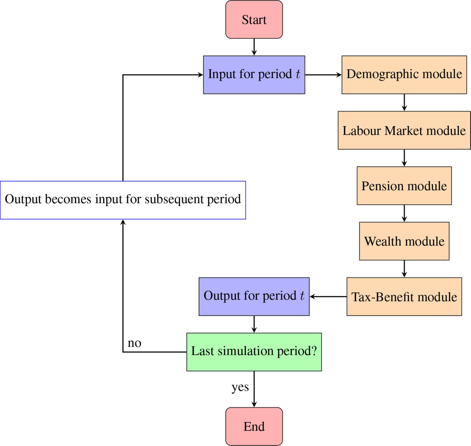
Modular structure of T-DYMM

Structure of the Labour Market module

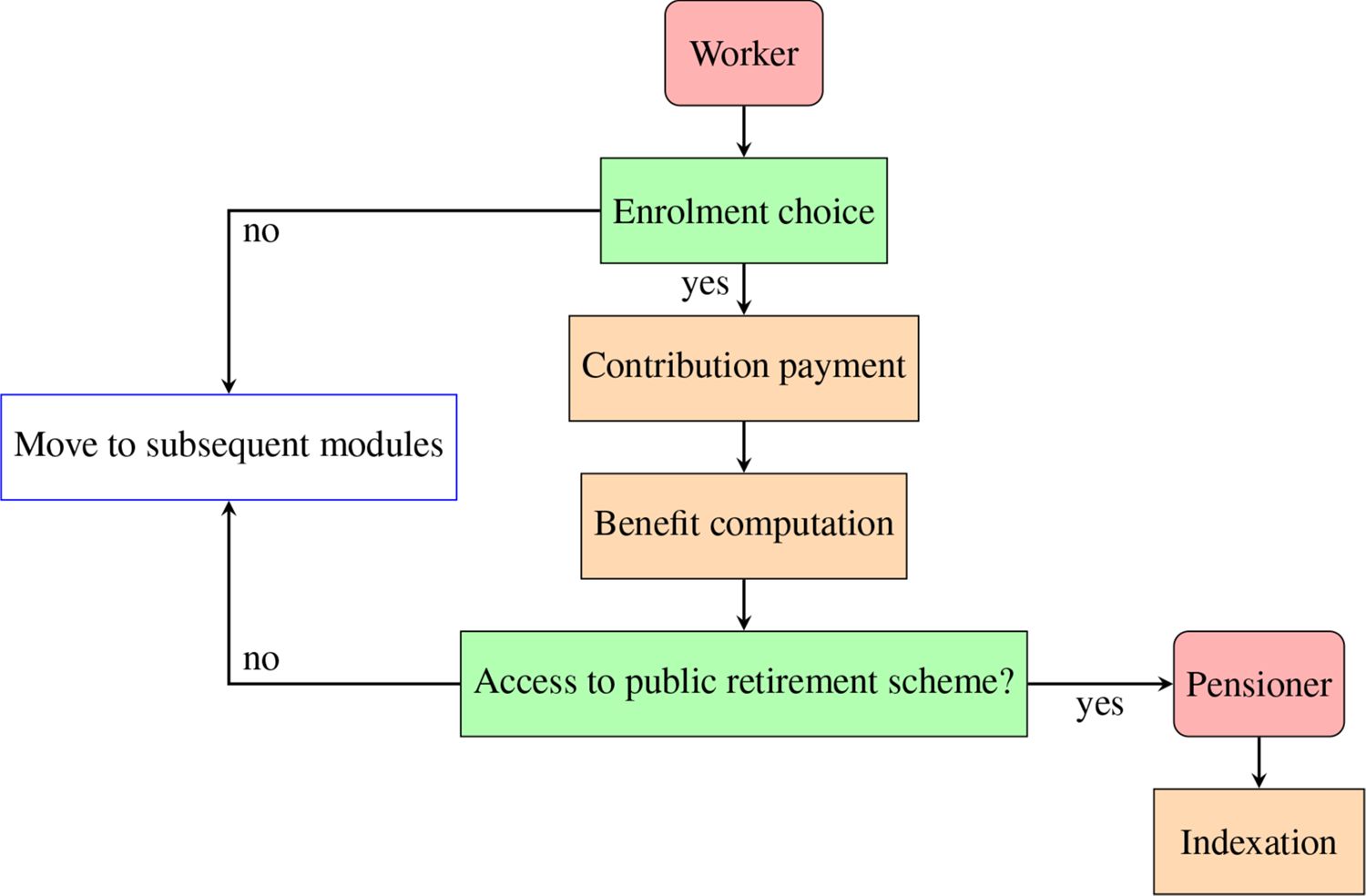
Structure of the Pension module, work-related public pensions (first pillar)
Structure of the Pension module, private pensions (second and third pillars)
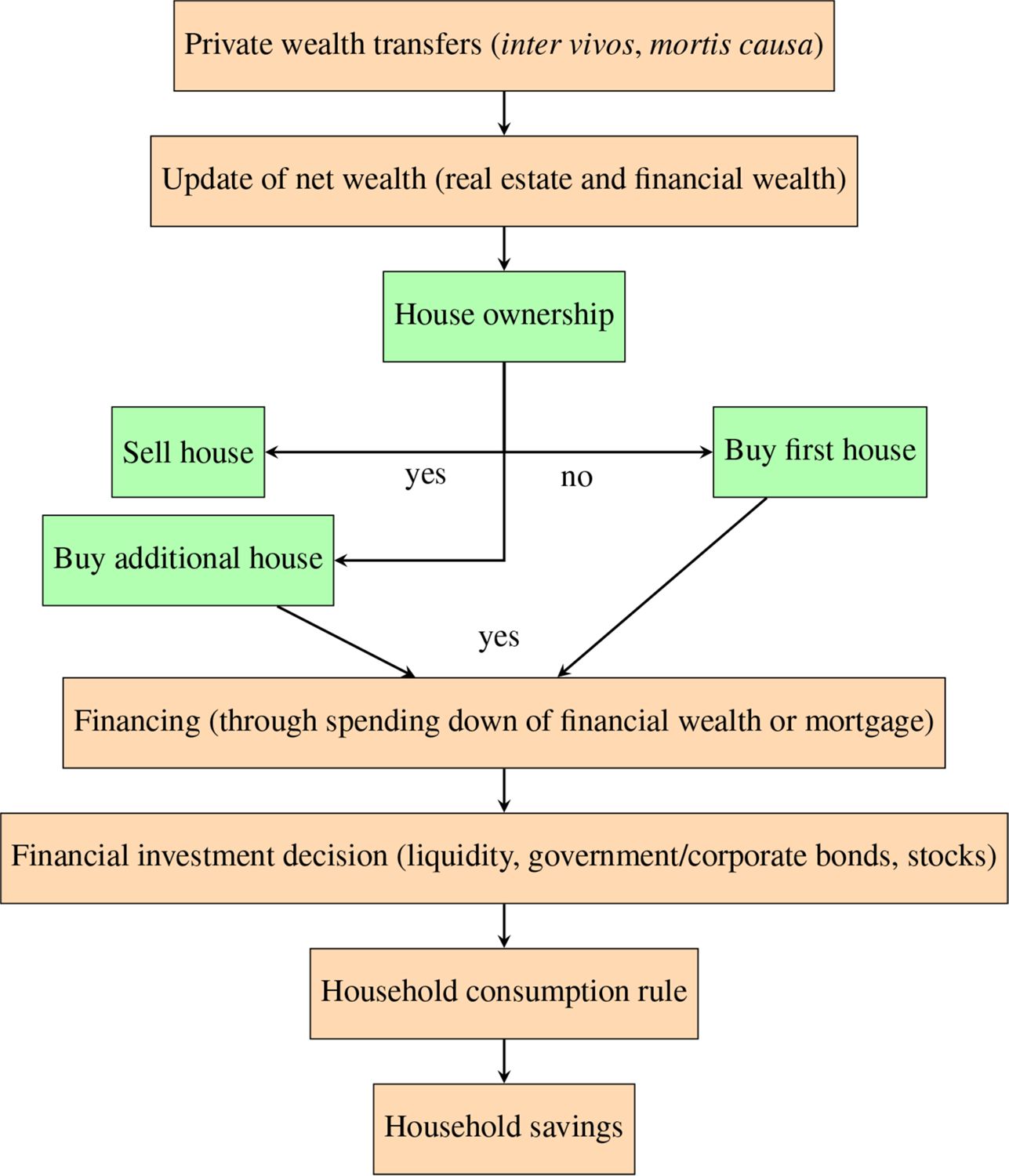
Structure of the Wealth module. Note: If individuals do not sell or buy a house, they move to financial investment decisions and subsequent processes.

Sample evolution, individuals and households. Note: Reference statistics for individuals are not reported since we align all dimensions that have an impact on the number of individuals in future years (i.e. fertility, mortality and migrations). For average members per household, in accordance with ISTAT, figures for period t are computed as the average of t and t-1 and rounded to the first decimal. Source: Authors’ elaborations of simulation results and ISTAT statistics.
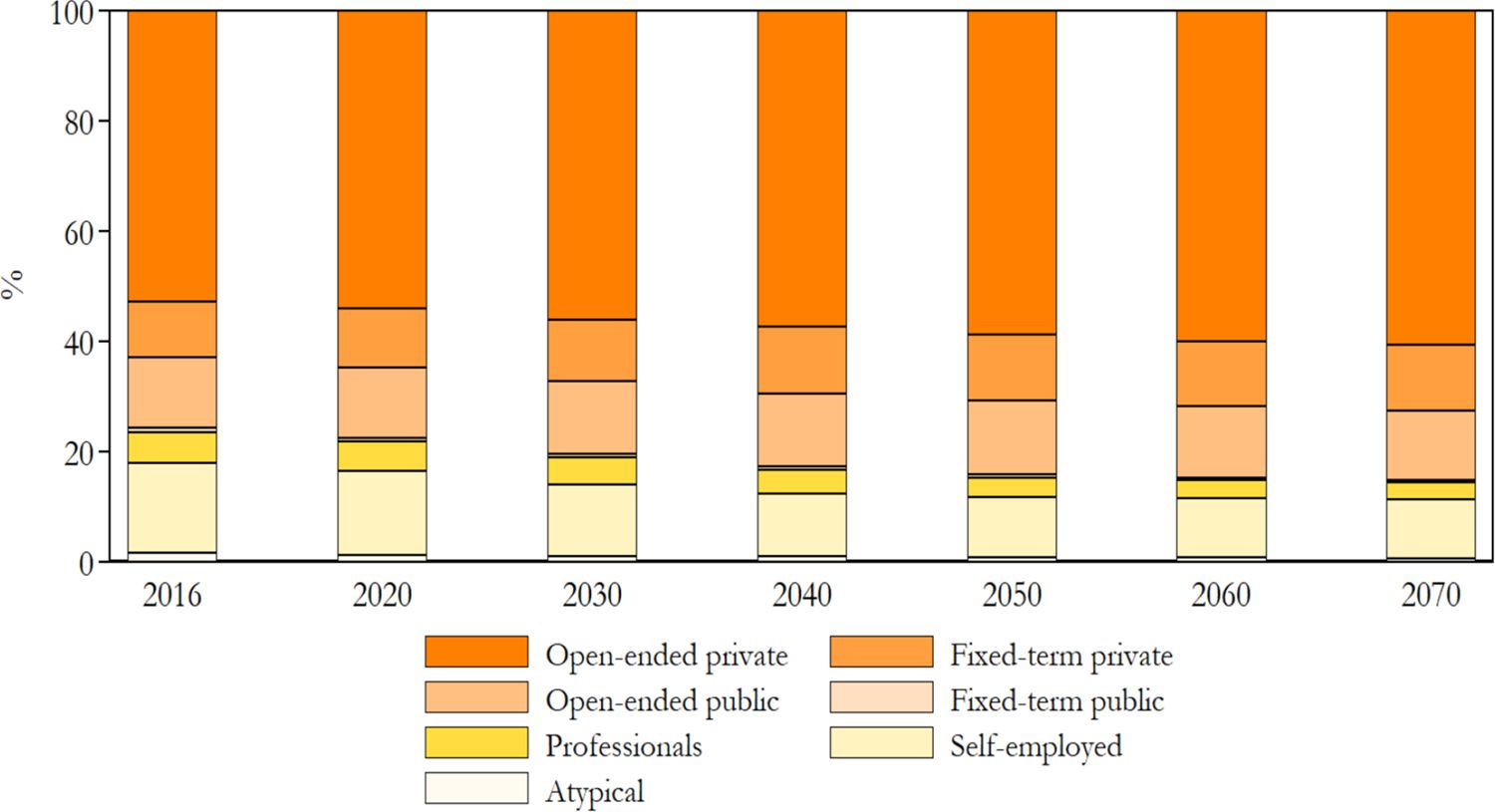
Repartition by work category. Note: Working pensioners are not considered. ISTAT statistics enable the validation of work categories at a more aggregate level compared with T-DYMM’s outputs. We observe that simulation results adhere almost perfectly to reference statistics in the period 2018–2020, while there are no disaggregated statistics for previous years. Further details are available upon request to the authors. Source: Authors’ elaborations of simulation results and ISTAT statistics.
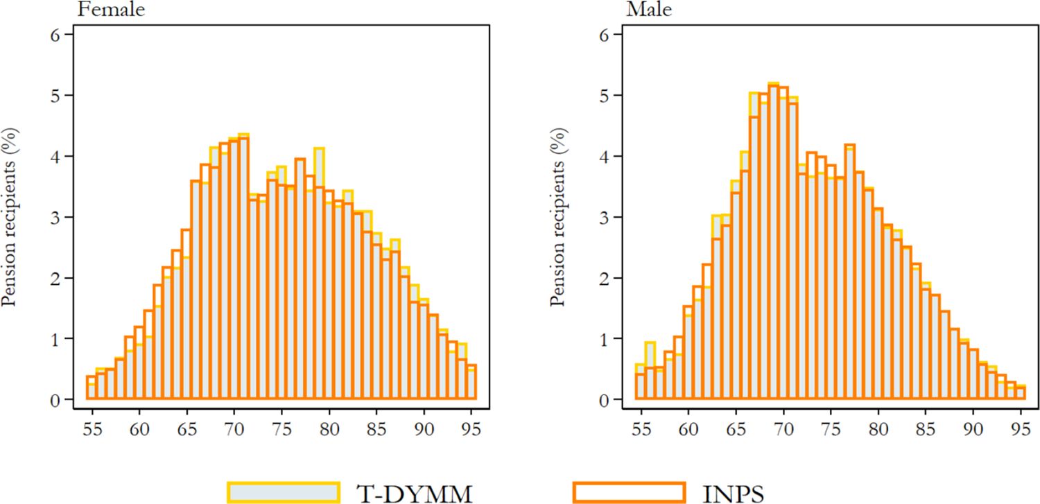
Old-age/seniority, survivor and incapacity pension recipients in 2017 by gender and age. Note: Individuals between ages 55 and 95 are included. The reference distribution is derived from INPS micro data on pensions (the same data employed for AD-SILC but relative to the last year available). Source: Authors’ elaborations of simulation results and INPS micro data.
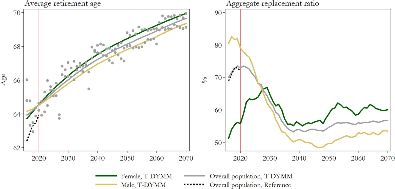
Average retirement age and aggregate replacement ratio by gender. Note: Lowess smoothing for T-DYMM average retirement ages excluding ‘Old age 3’ pensioners. The reference values for the average retirement age derive from the Italian State General Accounting Department (Ragioneria Generale dello Stato, RGS) statistics, while they refer to Eurostat statistics for the aggregate replacement ratio. Source: Authors’ elaborations of simulation results, RGS statistics and Eurostat statistics.

Wealth inequality and accumulation. Note: The reference net wealth amount is the sum of the following wealth components: dwellings, currency and deposits, debt securities, shares and other equity, derivatives, mutual fund shares and loans (negative value). See BI and ISTAT (2022) for further details. Gross income is the sum of gross income subject to PIT, self-employment income under substitute tax regimes and rental income that pays the cedolare secca. Source: Authors’ elaborations of simulation results, DF statistics and NA statistics.
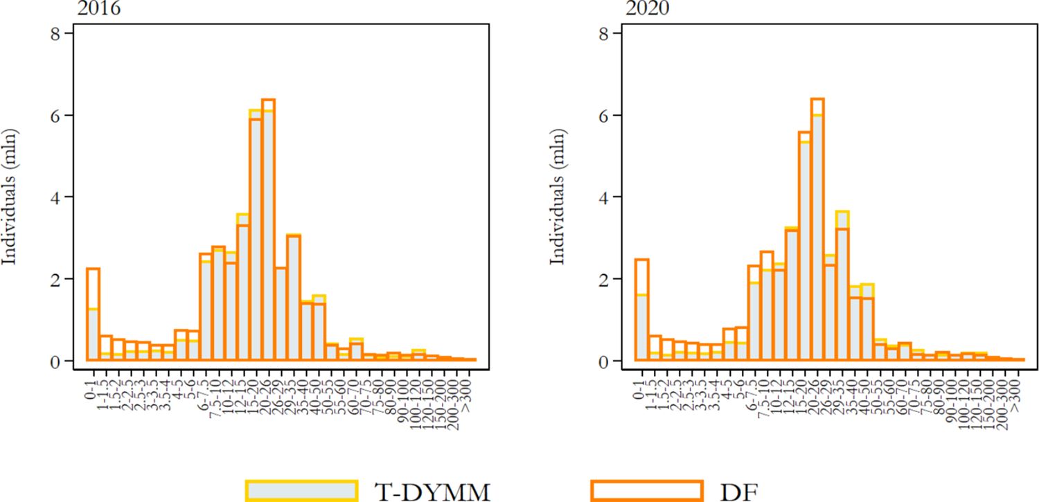
Frequency density function for gross income (values in thousands of euros on the horizontal axis). Note: Gross income is the sum of gross income subject to PIT and rental income subject to the cedolare secca. Source: Authors’ elaborations of simulation results and DF statistics.
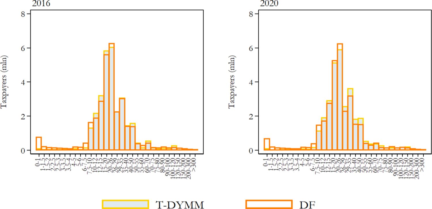
Distribution of PIT taxpayers by gross income group (values in thousands of euros on the horizontal axis). Note: Gross income is the sum of gross income subject to PIT and rental income subject to the cedolare secca. Source: Authors’ elaborations of simulation results and DF statistics.
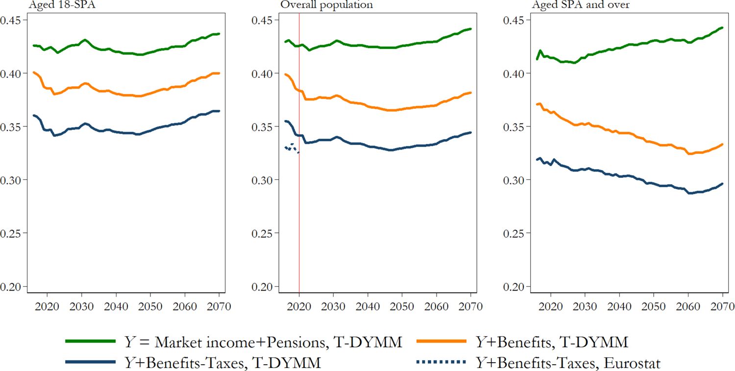
Gini index for equivalised income definitions by age group. Source: Authors’ elaborations of simulation results and Eurostat statistics.

At-risk-of-poverty rate by age group. Source: Authors’ elaborations of simulation results and Eurostat statistics.
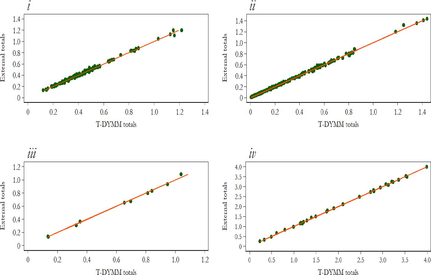
Distributions employed in the calibration of IT-SILC weights (individuals in millions on the horizontal axis). Note: i) distribution of the population at the macro-regional level by gender and fourteen age groups; ii) distribution of the population at the regional level by gender and five age groups; iii) distribution of the foreign population at the macro-regional level by gender; iv) distribution of the population at the macro-regional level by demographic size of the municipality of residence. Source: Authors’ elaborations of AD-SILC 2015 and ISTAT statistics.

Distribution of the population by gender and one-year age group (individuals in millions on the horizontal axis). Source: Authors’ elaborations of AD-SILC 2015 and ISTAT statistics.
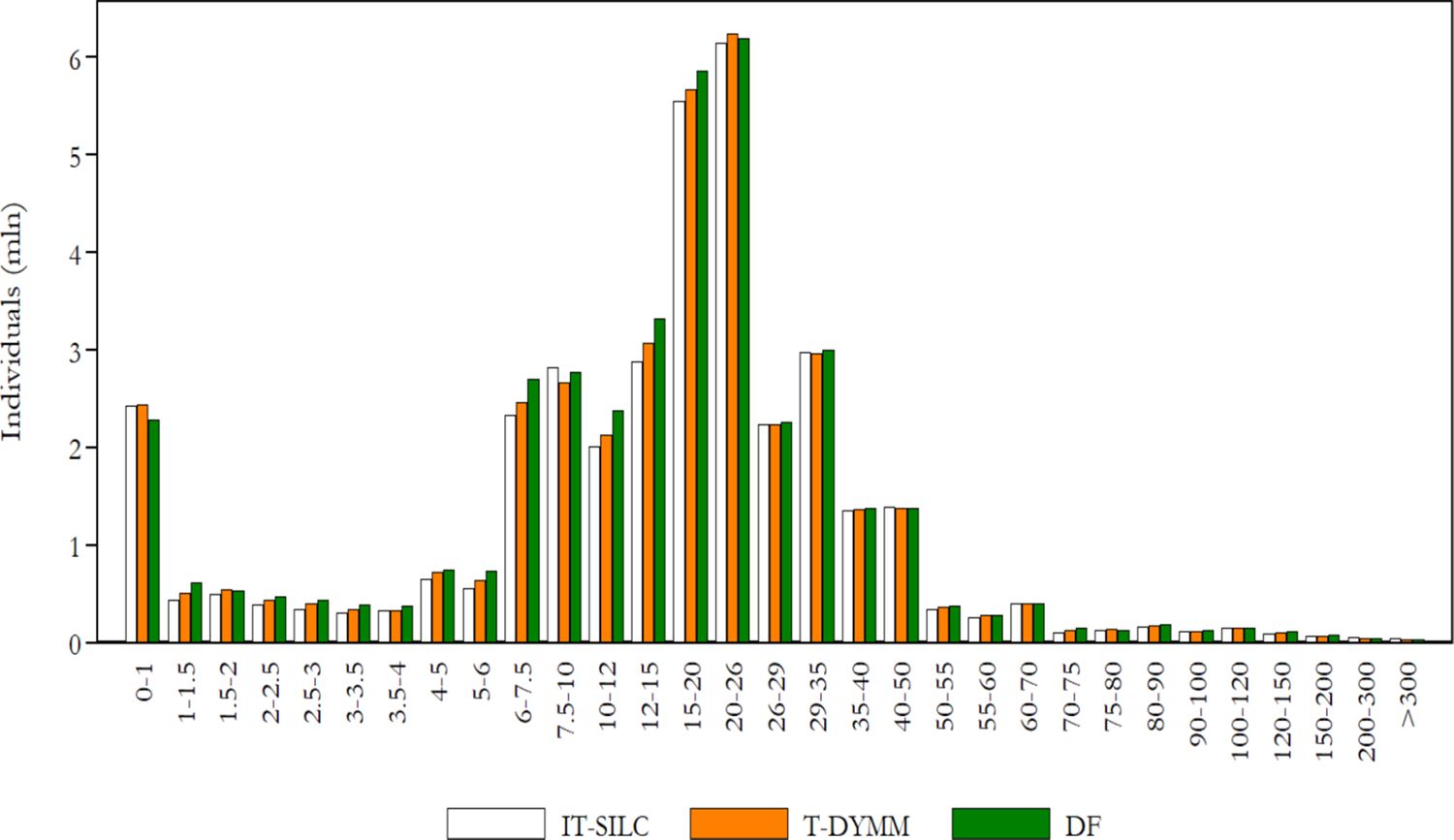
Frequency density function for gross income (values in thousands of euros on the horizontal axis). Note: Gross income is the sum of gross income subject to PIT and rental income subject to the cedolare secca. Source: Authors’ elaborations of AD-SILC 2015 and DF statistics.
Tables
Aligned processes in T-DYMM.
| Module | Process | Source |
|---|---|---|
| Demographic module | Fertility, mortality, immigration and emigration flows | ISTAT (historical data) and Eurostat - Europop 2019 projections |
| Education, age of exit from original household, informal and formal marriages, divorces | ISTAT and OECD (for education achievements of immigrants) | |
| Labour Market module | Employment rate, inflation growth, GDP growth, productivity growth | ISTAT (historical data) and European Commission 2022 Spring Forecasts and Working Group on Ageing Populations and Sustainability (AWG) assumptions |
| Take-up rate of unemployment benefits | INPS | |
| Quota of permanent public employees | ISTAT | |
| Pension module | Number of disability allowances and incapacity pensions | INPS |
| Enrolment in private pension plans | Italian Supervisory Authority on Pension funds (COVIP) | |
| Wealth module | Households that pay rent | Department of Finance |
| Returns on financial and housing assets | European Commission 2022 Spring Forecasts and AWG assumptions, Italian Housing Observatory (Osservatorio del Mercato Immobiliare, OMI) and Standard & Poor’s (S&P) 500 | |
| Houses sold and bought, average propensity to consume | ISTAT | |
| Tax-Benefit module | Beneficiaries of selected tax expenditures and substitute tax regimes | Department of Finance |
| Take-up rates of specific social assistance measures | INPS |
Eligibility requirements for retirement as simulated in T-DYMM.
| Criteria | Regime | Requirements | 2022 |
|---|---|---|---|
| Old age 1 | NDC | age | 64 years |
| seniority | 20 years | ||
| amount | 2.8*assegno sociale | ||
| Old age 2 | NDC, mixed | age | 67 years |
| NDC, mixed | seniority | 20 years | |
| NDC | amount | 1.5*assegno sociale | |
| Old age 3 | NDC | age | 71 years |
| seniority | 5 years | ||
| Seniority | NDC, mixed | seniority, males | 42 years, 6 months |
| seniority, females | 41 years, 6 months | ||
| Seniority - young workers | mixed | seniority | 41 years, 12 months accrued before turning 19 |
| Seniority - Quota 100/102 | mixed | age | 62/64 years |
| seniority | 38 years |
-
Note: The assegno sociale is the social allowance for the elderly. Since 2018, age requirements are aligned with ‘Old age 2’. Concerning ‘Old age 2’ seniority requirement, 15 years suffice for workers with at least 15 years of seniority as of Dec 31, 1992. For 2022, ‘Seniority - Quota 102’ replaces ‘Quota 100’ and the age requirement rises to 64.
Projected rate of nominal returns adopted in the Wealth module.
| Wealth component | Gain | 2016–2021 | 2022–2070 |
|---|---|---|---|
| House wealth | Income gain | OMI | Projections based on OMI |
| Government bonds | Income gain | Implicit rate of return on public debt, Italian Treasury Department | Implicit rate of return on public debt, EU Commission |
| Corporate bonds | Income gain | S&P 500 | Implicit rate of return on public debt, EU Commission |
| Capital gain | S&P 500 | Projections based on S&P 500* | |
| Stocks | Income gain | S&P 500 | Implicit rate of return on public debt, EU Commission |
| Capital gain | S&P 500 | Mark-up stocks–bonds* | |
| Mortgages | Long-term interest rate, Italian Treasury Department | Long-term interest rate, EU Commission |
-
*
For the 2022–2023 period a linear convergence is applied to ensure a smoother transition from historical data to long-term assumptions.
SICs and taxes simulated in T-DYMM.
| SICs |
|---|
| Employer social insurance contributions |
| Employee social insurance contributions |
| Contributions paid by self-employed workers |
| Proportional taxes and tax regimes that substitute the personal income tax for: |
| i) Capital income: government/corporate bonds and sharesa |
| ii) Private pensions: Pillars II and IIIb |
| iii) Self-employment income subject to substitute tax regimes (regime fiscale di vantaggioc or regime forfetariob) |
| iv) Rental income subject to cedolare secca (assigned to the head of the household)b |
| v) Productivity bonusesb |
| Personal income tax (Imposta sul reddito delle persone fisiche – IRPEF)d |
-
Note: The order of appearance follows the module sequence: a) The ‘Financial investment decision’ process is modelled through dynamic regressions based on SHIW data (see Section 3.4). b) Recipients are aligned with aggregate administrative data in the 2016–2020 interval, while from 2021 onwards we align recipients by taking as reference the external totals as of 2020 and updating them with: the population growth at the individual level for ii; the population growth of self-employed workers for iii; the population growth at the household level for iv; and the population growth of employees for v. c) Recipients are bound to gradually diminish to zero under current legislation. We assume that there are no recipients by 2030. d) Recipients of residual tax expenditures are aligned with external totals derived from tax return micro data for the 2015 tax period, annually updated to the population growth of recipients of gross income subject to PIT.
In-cash benefits simulated in T-DYMM.
| Unemployment benefits (NASpI and DIS-COLL)a,b |
| In-work bonus for employees and atypical workers (Bonus IRPEF, which has replaced Bonus 80 euro) |
| Means-tested disability allowances (Pensione di inabilità agli invalidi civili up to the standard pensionable age and Assegno sociale sostitutivo afterward)c |
| Non-means-tested disability allowances (Indennità di accompagnamento for those aged 18 or above and Indennità di frequenza for those aged under 18)c |
| War pensions and indemnity annuities (Rendite indennitarie)d |
| 14th month pensiond (Quattordicesima) |
| Social allowance for the elderly and related increases (Assegno sociale and Maggiorazioni sociali) |
| Increases to old-age/seniority, survivor and incapacity integrated pensions (Maggiorazioni sociali del minimo)e |
| Family allowances for employees’ and pensioners’ households (Assegni al nucleo familiare – ANF, up to 2021 for households with dependent children)f |
| Newborn bonus (Bonus bebè, up to 2021) |
| Mother bonus (Bonus mamma domani, from 2017 to 2021) |
| Universal unique allowance (Assegno unico e universale – AUU, from 2022 onwards)g,h |
| Minimum income schemes:b,h |
| - SIA (Sostegno all’inclusione attiva, 2017) |
| - REI (Reddito di inclusione, 2018) |
| - RdC (Reddito di cittadinanza, from 2019 onwards) |
-
Note: The order of appearance follows the module sequence. a) Unemployment benefits are actually simulated prior to the Tax-Benefit module because they are subject to the personal income tax. b) For the first two years of the simulation, administrative totals are employed for the alignments. From the latest available figures onwards, the ratio between actual (administrative data) and potential (obtained from T-DYMM’s simulations) recipients is kept constant. c) The average probabilities of receiving disability allowances are aligned by gender and five-year age group with the INPS statistics available for the period 2016–2020; beyond 2020, probabilities are projected following the same logic adopted for disability probabilities (which in turn follow the Reference Scenario of the 2021 Ageing Report). d) Recipients in T-DYMM’s base-year sample will hold these benefits until death. New occurrences are not simulated. e) Integrations to old-age/seniority, survivor and inability pensions (Integrazione al trattamento minimo) are included among pension benefits subject to PIT and thus not listed in the above table. f) ANF continue to be granted to households without children – but conditional to specific requirements in terms of household members and their disability status – following the introduction of AUU. g) The new allowance has replaced family allowances for employees’ and pensioners’ households, the newborn bonus, the mother bonus, family allowances granted at the municipal level (not simulated) and PIT tax credits for dependent children under the age of 21. h) In the simulation of AUU and minimium income schemes, we grant benefits for twelve months in a year following first introduction.
Comparison between sample totals and external totals for selected distributions.
| Variable | (1) IT-SILC totals | (2) T-DYMM totals | (3) External totals | (1)/(3) | (2)/(3) |
|---|---|---|---|---|---|
| Individuals | 60,323,126 | 60,631,408 | 60,665,551 | 0.994 | 0.999 |
| Households (in thousands) | 25,821 | 25,429 | 25,386 | 1.017 | 1.002 |
| Ratio individuals/households | 2.336 | 2.384 | 2.390 | 0.977 | 0.998 |
| Foreign population by gender, area of birth and educational attainment: | |||||
| Female – EU – Upper secondary | 566,866 | 540,119 | 532,951 | 1.064 | 1.013 |
| Female – EU – Tertiary | 140,621 | 186,397 | 194,004 | 0.725 | 0.961 |
| Female – non-EU – Upper secondary | 689,547 | 706,173 | 695,296 | 0.992 | 1.016 |
| Female – non-EU – Tertiary | 311,078 | 307,186 | 302,485 | 1.028 | 1.016 |
| Male – EU – Upper secondary | 287,465 | 334,650 | 345,220 | 0.833 | 0.969 |
| Male – EU – Tertiary | 93,373 | 61,285 | 63,090 | 1.480 | 0.971 |
| Male – non-EU – Upper secondary | 609,550 | 572,669 | 573,095 | 1.064 | 0.999 |
| Male – non-EU – Tertiary | 151,188 | 205,723 | 206,235 | 0.733 | 0.998 |
| Population by number of household members (in thousands): | |||||
| 1 | 8,369 | 8,032 | 8,016 | 1.044 | 1.002 |
| 2 | 14,332 | 13,866 | 13,838 | 1.036 | 1.002 |
| 3 | 15,141 | 15,043 | 15,111 | 1.002 | 0.995 |
| 4 | 16,112 | 16,075 | 16,200 | 0.995 | 0.992 |
| 5 | 4,890 | 5,400 | 5,290 | 0.924 | 1.021 |
| 6 or more | 1,478 | 2,214 | 2,211 | 0.668 | 1.001 |
| Individuals with retirement income at the macro-regional level by gender: | |||||
| North West – Female | 2,218,088 | 2,367,979 | 2,378,635 | 0.933 | 0.996 |
| North East – Female | 1,546,322 | 1,675,793 | 1,675,812 | 0.923 | 1 |
| Middle – Female | 1,599,179 | 1,667,401 | 1,671,085 | 0.957 | 0.998 |
| South – Female | 1,701,624 | 1,753,352 | 1,766,032 | 0.964 | 0.993 |
| Islands – Female | 834,713 | 835,608 | 832,585 | 1.003 | 1.004 |
| North West – Male | 1,993,336 | 2,033,838 | 2,059,497 | 0.968 | 0.988 |
| North East – Male | 1,473,823 | 1,498,042 | 1,479,615 | 0.996 | 1.012 |
| Middle – Male | 1,443,607 | 1,485,073 | 1,486,315 | 0.971 | 0.999 |
| South – Male | 1,608,304 | 1,593,656 | 1,616,762 | 0.995 | 0.986 |
| Islands – Male | 796,957 | 787,546 | 795,288 | 1.002 | 0.990 |
| Individuals with retirement income by gender and six age groups: | |||||
| Female – 0-54 | 564,506 | 600,895 | 604,675 | 0.934 | 0.994 |
| Female – 55-64 | 1,023,141 | 1,067,015 | 1,072,665 | 0.954 | 0.995 |
| Female – 65-69 | 1,443,927 | 1,487,870 | 1,488,105 | 0.970 | 1 |
| Female – 70-74 | 1,208,479 | 1,276,298 | 1,269,707 | 0.952 | 1.005 |
| Female – 75-79 | 1,264,050 | 1,348,517 | 1,364,252 | 0.927 | 0.988 |
| Female – 80 and over | 2,395,823 | 2,519,538 | 2,524,745 | 0.949 | 0.998 |
| Male – 0-54 | 741,462 | 694,984 | 711,781 | 1.042 | 0.976 |
| Male – 0-54 | 741,462 | 694,984 | 711,781 | 1.042 | 0.976 |
| Male – 65-69 | 1,606,143 | 1,605,099 | 1,607,490 | 0.999 | 0.999 |
| Male – 70-74 | 1,262,353 | 1,271,212 | 1,301,312 | 0.970 | 0.977 |
| Male – 75-79 | 1,175,818 | 1,227,220 | 1,218,628 | 0.965 | 1.007 |
| Male – 80 and over | 1,392,296 | 1,469,307 | 1,472,586 | 0.945 | 0.998 |
| Individuals with retirement income by gender and type of pension: | |||||
| Female – Old-age and seniority pensions | 4,709,966 | 5,204,113 | 5,196,325 | 0.906 | 1.001 |
| Female – Inability pensions | 565,080 | 617,424 | 624,406 | 0.905 | 0.989 |
| Female – Survivors’ pensions | 3,605,291 | 4,034,618 | 4,032,187 | 0.894 | 1.001 |
| Female – Disability pensions | 1,416,051 | 1,813,111 | 1,824,118 | 0.776 | 0.994 |
| Female – Social pension | 518,856 | 536,305 | 541,679 | 0.958 | 0.990 |
| Male – Old-age and seniority pensions | 5,716,676 | 6,319,952 | 6,377,756 | 0.896 | 0.991 |
| Male – Inability pensions | 606,074 | 642,345 | 652,098 | 0.929 | 0.985 |
| Male – Survivors’ pensions | 583,017 | 603,947 | 617,234 | 0.945 | 0.978 |
| Male – Disability pensions | 992,888 | 1,201,027 | 1,219,673 | 0.814 | 0.985 |
| Male – Social pension | 266,998 | 297,015 | 304,413 | 0.877 | 0.976 |
| Retired workers by gender (in thousands): | |||||
| Female | 196 | 115 | 111 | 1.766 | 1.036 |
| Male | 536 | 321 | 331 | 1.619 | 0.970 |
| In-work individuals by area of birth (in thousands): | |||||
| Italy | 20,107 | 20,132 | 20,106 | 1 | 1.001 |
| EU or non-EU | 3,033 | 2,326 | 2,359 | 1.286 | 0.986 |
| In-work individuals by employment status (in thousands): | |||||
| Employees | 18,042 | 17,008 | 16,988 | 1.062 | 1.001 |
| Freelancers | 1,161 | 1,314 | 1,327 | 0.875 | 0.990 |
| Craftsmen, traders and farmers | 3,387 | 3,793 | 3,801 | 0.891 | 0.998 |
| Atypical workers (co.co.co.) | 550 | 344 | 349 | 1.576 | 0.986 |
| Employees by type of contract (in thousands): | |||||
| Open-ended | 15,290 | 14,615 | 14,605 | 1.047 | 1.001 |
| Fixed-term | 2,752 | 2,393 | 2,383 | 1.155 | 1.004 |
| Full-time | 14,324 | 13,634 | 13,642 | 1.050 | 0.999 |
| Part-time | 3,718 | 3,373 | 3,346 | 1.111 | 1.008 |
| Population by gender and civil status: | |||||
| Female – Single | 11,444,708 | 11,878,040 | 11,900,653 | 0.962 | 0.998 |
| Female – Married or separated | 14,719,913 | 14,669,927 | 14,683,481 | 1.002 | 0.999 |
| Female – Divorced | 824,754 | 862,563 | 871,345 | 0.947 | 0.990 |
| Female – Widow | 4,022,839 | 3,753,115 | 3,753,751 | 1.072 | 1 |
| Male – Single | 13,305,714 | 13,646,650 | 13,641,747 | 0.975 | 1 |
| Male – Married or separated | 14,586,291 | 14,448,378 | 14,485,092 | 1.007 | 1 |
| Male – Divorced | 477,936 | 579,280 | 584,343 | 0.818 | 0.991 |
| Households at the regional level (in thousands): | |||||
| Male – Widower | 940,970 | 752,454 | 745,139 | 1.263 | 1.010 |
| Piemonte | 2,008 | 1,963 | 1,950 | 1.030 | 1.007 |
| Valle d’Aosta | 61 | 125 | 62 | 0.984 | 2.016 |
| Liguria | 771 | 788 | 756 | 1.020 | 1.042 |
| Lombardia | 4,418 | 4,299 | 4,222 | 1.046 | 1.018 |
| Bolzano | 217 | 246 | 215 | 1.009 | 1.144 |
| Trento | 233 | 254 | 228 | 1.022 | 1.114 |
| Veneto | 2,059 | 2,022 | 1,983 | 1.038 | 1.020 |
| Friuli-Venezia Giulia | 559 | 622 | 544 | 1.028 | 1.143 |
| Emilia-Romagna | 1,993 | 1,928 | 1,961 | 1.016 | 0.983 |
| Toscana | 1,643 | 1,614 | 1,636 | 1.004 | 0.987 |
| Umbria | 383 | 420 | 379 | 1.011 | 1.108 |
| Marche | 644 | 683 | 641 | 1.005 | 1.066 |
| Lazio | 2,631 | 2,528 | 2,601 | 1.012 | 0.972 |
| Abruzzo | 555 | 532 | 549 | 1.011 | 0.969 |
| Molise | 131 | 167 | 131 | 1 | 1.275 |
| Campania | 2,157 | 2,068 | 2,173 | 0.993 | 0.952 |
| Puglia | 1,587 | 1,549 | 1,593 | 0.996 | 0.972 |
| Basilicata | 231 | 248 | 238 | 0.971 | 1.042 |
| Calabria | 800 | 740 | 806 | 0.993 | 0.918 |
| Sicilia | 2,022 | 1,930 | 2,022 | 1 | 0.955 |
| Sardegna | 719 | 699 | 696 | 1.033 | 1.004 |
| Households by type (in thousands): | |||||
| Single | 8,369 | 8,175 | 8,312 | 1.007 | 0.984 |
| Single with children | 2,216 | 2,083 | 2,360 | 0.939 | 0.883 |
| Couple | 5,142 | 4,973 | 5,110 | 1.006 | 0.973 |
| Couple with children | 8,692 | 8,701 | 8,754 | 0.993 | 0.994 |
| Other | 1,403 | 1,494 | 850 | 1.651 | 1.758 |
-
Source: Authors’ elaborations of AD-SILC 2015 and statistics from different institutes (Eurostat, ISTAT, INPS and DF).
Probability of being employed.
| Male | Female | |||
|---|---|---|---|---|
| b | se | b | se | |
| extra-EU born | 0.318*** | (0.042) | 0.250*** | (0.038) |
| studying | -1.022*** | (0.033) | -1.029*** | (0.033) |
| retired | -1.327*** | (0.049) | -1.209*** | (0.069) |
| age | 0.383*** | (0.012) | 0.064*** | (0.005) |
| age2 | -0.010*** | (0.000) | -0.001*** | (0.000) |
| age3 | 0.000*** | (0.000) | ||
| upper sec. degree | 0.250*** | (0.020) | 0.385*** | (0.021) |
| tertiary degree | 0.578*** | (0.032) | 0.850*** | (0.031) |
| disabled | -0.335*** | (0.050) | -0.306*** | (0.058) |
| disability pension | -1.048*** | (0.100) | -1.030*** | (0.096) |
| disability allowance | -1.021*** | (0.125) | -0.864*** | (0.131) |
| incapacity pension | -1.018*** | (0.086) | -1.285*** | (0.138) |
| in couple | 0.107*** | (0.027) | -0.318*** | (0.033) |
| partner working (lag) | 0.204*** | (0.027) | 0.156*** | (0.030) |
| experience | 0.085*** | (0.003) | 0.098*** | (0.004) |
| experience2 | -0.001*** | (0.000) | -0.002*** | (0.000) |
| last spell duration (out-of-work) | -0.199*** | (0.007) | -0.201*** | (0.007) |
| last spell duration (working) | 0.027*** | (0.001) | 0.031*** | (0.002) |
| pen-ended private (lag) | 3.439*** | (0.034) | 3.666*** | (0.036) |
| fixed-term private (lag) | 2.783*** | (0.038) | 3.028*** | (0.038) |
| pen-ended public (lag) | 3.760*** | (0.058) | 4.506*** | (0.063) |
| fixed-term public (lag) | 2.969*** | (0.125) | 3.549*** | (0.084) |
| professional (lag) | 4.470*** | (0.101) | 4.133*** | (0.125) |
| self-employed (lag) | 4.082*** | (0.053) | 4.415*** | (0.068) |
| atypical (lag) | 3.600*** | (0.071) | 3.144*** | (0.070) |
| children aged 0-6 | -0.376*** | (0.030) | ||
| constant | -5.725*** | (0.163) | -2.242*** | (0.101) |
| pseudo-R2 | 0.719 | 0.739 | ||
| no. of observations | 253,274 | 250,143 | ||
-
Note: Significance levels are indicated by * < .1, ** < .05, *** < .01. The omitted category for the educational level is compulsory education. Experience refers to years of work. Children aged 0-6 is equal to one when children in that age group are present. All other variables except for age and duration in last spell are dummies. Source: Authors’ elaborations on AD-SILC data.
Probability of being employed in each employment category for males.
| Fixed-term employee | Professionals | Self-employed | Atypical | |||||
|---|---|---|---|---|---|---|---|---|
| b | se | b | se | b | se | b | se | |
| EU born | 0.095 | (0.082) | -0.785** | (0.362) | -0.016 | (0.148) | -0.218 | (0.242) |
| extra-EU born | 0.123** | (0.050) | -0.817*** | (0.227) | -0.049 | (0.102) | -0.403*** | (0.145) |
| age | -0.024*** | (0.009) | 0.227*** | (0.028) | 0.078*** | (0.015) | 0.097*** | (0.019) |
| age2 | 0.000*** | (0.000) | -0.002*** | (0.000) | -0.001*** | (0.000) | -0.001*** | (0.000) |
| upper sec. degree | -0.336*** | (0.029) | 1.407*** | (0.148) | 0.068 | (0.050) | 0.392*** | (0.072) |
| tertiary degree | -0.494*** | (0.043) | 1.902*** | (0.162) | -0.275*** | (0.076) | 0.745*** | (0.094) |
| studying | 0.403*** | (0.054) | 0.156 | (0.180) | -0.356*** | (0.106) | 0.844*** | (0.110) |
| in couple | -0.214*** | (0.032) | -0.329*** | (0.103) | 0.019 | (0.056) | -0.063 | (0.076) |
| exp. as open-ended | -0.060*** | (0.006) | -0.191*** | (0.017) | -0.061*** | (0.010) | -0.097*** | (0.012) |
| exp. as fixed-term | 0.143*** | (0.016) | -0.321*** | (0.089) | -0.186*** | (0.032) | -0.266*** | (0.058) |
| exp. as atypical | 0.012 | (0.021) | 0.081* | (0.046) | -0.053* | (0.028) | 0.392*** | (0.024) |
| exp. as self-employed | 0.026*** | (0.009) | -0.025 | (0.026) | 0.174*** | (0.009) | 0.072*** | (0.013) |
| exp. as professional | -0.068*** | (0.020) | 0.267*** | (0.019) | -0.010 | (0.029) | 0.020 | (0.024) |
| exp.2 as open-ended | 0.000 | (0.000) | 0.003*** | (0.001) | 0.000 | (0.000) | 0.001*** | (0.000) |
| exp.2 as fixed-term | 0.005*** | (0.002) | 0.019 | (0.013) | 0.018*** | (0.003) | 0.017*** | (0.006) |
| exp.2 as atypical | -0.003 | (0.002) | -0.004 | (0.003) | 0.005** | (0.002) | -0.013*** | (0.002) |
| exp.2 as self-employed | -0.001*** | (0.000) | -0.002 | (0.001) | -0.004*** | (0.000) | -0.002*** | (0.000) |
| exp.2 as professional | 0.001 | (0.001) | -0.006*** | (0.001) | -0.001 | (0.001) | -0.000 | (0.001) |
| pen-ended (lag) | -2.813*** | (0.041) | -3.589*** | (0.153) | -3.038*** | (0.072) | -3.735*** | (0.107) |
| fixed-term (lag) | 0.989*** | (0.040) | -1.620*** | (0.216) | -1.401*** | (0.103) | -1.219*** | (0.138) |
| professional (lag) | -0.373** | (0.190) | 4.160*** | (0.139) | 0.083 | (0.231) | -0.006 | (0.222) |
| self-employed (lag) | 0.226** | (0.097) | 0.047 | (0.267) | 4.861*** | (0.082) | 1.043*** | (0.120) |
| atypical (lag) | -0.023 | (0.107) | 0.727*** | (0.184) | 0.874*** | (0.116) | 2.752*** | (0.097) |
| constant | 0.317* | (0.166) | -8.894*** | (0.546) | -3.057*** | (0.284) | -5.095*** | (0.371) |
| pseudo-R2 | 0.732 | |||||||
| no. of observations | 140,331 | |||||||
-
Note: Significance levels are indicated by * < .1, ** < .05, *** < .01. The omitted category in the dependent variable is open-ended employee. The omitted category for the nationality is Italian, while for the educational level, it is compulsory education. Exp. refers to years of work. All other variables except for age are dummies. Coefficients in units of log odds. Source: Authors’ elaborations of AD-SILC data.
Probability of being employed in each employment category for females.
| Fixed-term employee | Professionals | Self-employed | Atypical | |||||
|---|---|---|---|---|---|---|---|---|
| b | se | b | se | b | se | b | se | |
| EU born | -0.045 | (0.071) | -0.644*** | (0.248) | -0.418** | (0.165) | -0.357** | (0.164) |
| extra-EU born | -0.147*** | (0.054) | -0.747*** | (0.231) | -0.339*** | (0.125) | -0.475*** | (0.131) |
| age | 0.039*** | (0.010) | 0.249*** | (0.036) | 0.078*** | (0.021) | 0.089*** | (0.019) |
| age2 | -0.001*** | (0.000) | -0.003*** | (0.000) | -0.001*** | (0.000) | -0.001*** | (0.000) |
| upper sec. degree | -0.310*** | (0.032) | 0.995*** | (0.184) | -0.005 | (0.070) | 0.172** | (0.073) |
| tertiary degree | -0.439*** | (0.041) | 2.117*** | (0.185) | -0.604*** | (0.098) | 0.634*** | (0.085) |
| studying | 0.362*** | (0.056) | -0.158 | (0.179) | -0.252* | (0.137) | 0.720*** | (0.095) |
| in couple | 0.064* | (0.034) | -0.242** | (0.117) | 0.312*** | (0.074) | -0.116 | (0.071) |
| children aged 0-6 | -0.085** | (0.040) | -0.161 | (0.139) | 0.160* | (0.085) | -0.187** | (0.086) |
| exp. as open-ended | -0.044*** | (0.006) | -0.122*** | (0.022) | -0.028** | (0.013) | -0.048*** | (0.014) |
| exp. as fixed-term | 0.149*** | (0.015) | -0.351*** | (0.094) | -0.310*** | (0.042) | -0.249*** | (0.049) |
| exp. as atypical | 0.012 | (0.020) | 0.041 | (0.054) | -0.127*** | (0.041) | 0.353*** | (0.027) |
| exp. as self-employed | 0.043*** | (0.011) | -0.001 | (0.035) | 0.160*** | (0.013) | 0.052*** | (0.020) |
| exp. as professional | -0.020 | (0.021) | 0.309*** | (0.025) | -0.008 | (0.052) | -0.031 | (0.035) |
| exp.2 as open-ended | -0.000 | (0.000) | 0.002* | (0.001) | -0.001*** | (0.001) | -0.001 | (0.001) |
| exp.2 as fixed-term | 0.001 | (0.001) | 0.015 | (0.013) | 0.025*** | (0.004) | 0.015*** | (0.005) |
| exp.2 as atypical | -0.002 | (0.002) | -0.004 | (0.004) | 0.006* | (0.003) | -0.015*** | (0.002) |
| exp.2 as self-employed | -0.002*** | (0.000) | -0.000 | (0.001) | -0.004*** | (0.000) | -0.001* | (0.001) |
| exp.2 as professional | 0.001 | (0.001) | -0.008*** | (0.001) | -0.002 | (0.003) | -0.000 | (0.001) |
| pen-ended (lag) | -3.319*** | (0.043) | -4.417*** | (0.201) | -3.419*** | (0.096) | -4.158*** | (0.109) |
| fixed-term (lag) | 0.990*** | (0.041) | -1.562*** | (0.206) | -1.179*** | (0.130) | -1.056*** | (0.110) |
| professional (lag) | -0.122 | (0.192) | 4.112*** | (0.163) | 0.214 | (0.337) | 0.726*** | (0.219) |
| self-employed (lag) | 0.120 | (0.130) | 0.213 | (0.325) | 5.234*** | (0.113) | 0.258 | (0.181) |
| atypical (lag) | -0.233*** | (0.090) | 0.288* | (0.172) | 0.172 | (0.160) | 2.215*** | (0.088) |
| constant | -0.480*** | (0.186) | -7.982*** | (0.702) | -3.335*** | (0.395) | -4.213*** | (0.359) |
| pseudo-R2 | 0.699 | |||||||
| no. of observations | 110,553 | |||||||
-
Note: Significance levels are indicated by * < .1, ** < .05, *** < .01. The omitted category in the dependent variable is open-ended employee. The omitted category for the nationality is Italian, for the educational level it is compulsory education. Exp. refers to the experience in the labour market. All other variables except for age are dummies. Coefficients in units of log odds. Source: Authors’ elaborations of AD-SILC data.
Probability of being employed in each employment category for working pensioners.
| Open-ended private | Fixed-term private | Professional | Atypical | |||||
|---|---|---|---|---|---|---|---|---|
| b | se | b | se | b | se | b | se | |
| partner working | -0.800*** | (0.181) | -0.769*** | (0.230) | -1.620*** | (0.378) | -0.705*** | (0.175) |
| exp. as open-ended private | 0.086*** | (0.019) | 0.061*** | (0.023) | -0.031 | (0.031) | 0.002 | (0.021) |
| exp. as fixed-term private | 2.251*** | (0.521) | 3.048*** | (0.536) | 2.009*** | (0.611) | 1.829*** | (0.537) |
| exp. as atypical | -0.017 | (0.077) | 0.094 | (0.079) | 0.245*** | (0.092) | 0.808*** | (0.051) |
| exp. as self-employed | -0.123*** | (0.018) | -0.179*** | (0.021) | -0.324*** | (0.036) | -0.207*** | (0.018) |
| exp. as professional | -0.231 | (0.249) | -0.176 | (0.254) | 0.782*** | (0.133) | 0.178 | (0.128) |
| exp.2 as open-ended private | -0.001** | (0.000) | -0.001** | (0.001) | 0.000 | (0.001) | -0.000 | (0.001) |
| exp.2 as fixed-term private | -0.147*** | (0.029) | -0.177*** | (0.030) | -0.129*** | (0.036) | -0.118*** | (0.033) |
| exp.2 as atypical | -0.002 | (0.004) | -0.005 | (0.005) | -0.013** | (0.005) | -0.032*** | (0.003) |
| exp.2 as self-employed | 0.001 | (0.000) | 0.002*** | (0.000) | 0.004*** | (0.001) | 0.002*** | (0.000) |
| exp.2 as professional | 0.006 | (0.005) | 0.003 | (0.005) | -0.014*** | (0.003) | -0.002 | (0.003) |
| constant | -0.279 | (0.309) | -0.927** | (0.415) | -0.048 | (0.445) | -0.182 | (0.323) |
| pseudo-R2 | 0.581 | |||||||
| no. of observations | 9,627 | |||||||
-
Note: Significance levels are indicated by * < .1, ** < .05, *** < .01. The omitted category in the dependent variable is self-employed. Exp. refers to years of work. Partner working is a dummy. Coefficients in units of log odds. Source: Authors’ elaborations of AD-SILC data.
Monthly wages of private employees.
| Male | Female | |||||
|---|---|---|---|---|---|---|
| b | se | b | se | |||
| EU born | -0.033** | (0.013) | -0.235*** | (0.014) | ||
| extra-EU born | -0.102*** | (0.008) | -0.308*** | (0.011) | ||
| upper sec. degree | 0.126*** | (0.004) | 0.126*** | (0.005) | ||
| tertiary degree | 0.334*** | (0.008) | 0.277*** | (0.008) | ||
| children aged 0-3 | 0.035*** | (0.004) | -0.051*** | (0.005) | ||
| children aged 4 and over | 0.024*** | (0.004) | -0.047*** | (0.005) | ||
| exp. as private employee | 0.037*** | (0.001) | 0.025*** | (0.001) | ||
| exp.2 as private employee | -0.001*** | (0.000) | -0.000*** | (0.000) | ||
| pen-ended contract | 0.034*** | (0.005) | ||||
| part-time | -0.563*** | (0.010) | -0.403*** | (0.005) | ||
| partner working | 0.024*** | (0.003) | 0.016*** | (0.004) | ||
| constant | 7.169*** | (0.008) | 7.145*** | (0.008) | ||
| _u | 0.375 | 0.369 | ||||
| _e | 0.152 | 0.144 | ||||
| 0.860 | 0.868 | |||||
| R2-within | 0.142 | 0.192 | ||||
| R2-between | 0.460 | 0.396 | ||||
| R2-overall | 0.438 | 0.391 | ||||
| no. of observations | 88,966 | 63,934 | ||||
-
Note: Significance levels are indicated by * < .1, ** < .05, *** < .01. The omitted category for the nationality is Italian, while for the educational level it is compulsory education. Exp. refers to years of work. Children aged 0-3 or 4 and over is equal to one when children in that age group are present. All other variables are dummies. Source: Authors’ elaborations of AD-SILC data.
Monthly wages of public employees.
| Male | Female | |||||
|---|---|---|---|---|---|---|
| b | se | b | se | |||
| upper sec. degree | 0.091*** | (0.015) | 0.073*** | (0.012) | ||
| tertiary degree | 0.431*** | (0.018) | 0.242*** | (0.013) | ||
| exp. as public employee | 0.026*** | (0.002) | 0.024*** | (0.002) | ||
| exp.2 as public employee | -0.000*** | (0.000) | -0.000*** | (0.000) | ||
| children aged 0-3 | 0.048* | (0.025) | -0.067*** | (0.014) | ||
| children aged 4 and over | 0.060*** | (0.014) | -0.033*** | (0.009) | ||
| pen-ended contract | 0.254*** | (0.029) | 0.222*** | (0.017) | ||
| part-time | -0.437*** | (0.042) | -0.348*** | (0.018) | ||
| constant | 7.198*** | (0.030) | 7.159*** | (0.022) | ||
| _u | 0.473 | 0.366 | ||||
| _e | 0.341 | 0.266 | ||||
| 0.658 | 0.654 | |||||
| R2-within | 0.034 | 0.019 | ||||
| R2-between | 0.229 | 0.288 | ||||
| R2-overall | 0.209 | 0.260 | ||||
| no. of observations | 16,637 | 24,175 | ||||
-
Note: Significance levels are indicated by * < .1, ** < .05, *** < .01. The omitted category for the educational level is compulsory education. Exp. refers to years of work. Children aged 0-3 or 4 and over is equal to one when children in that age group are present. All other variables are dummies. Source: Authors’ elaborations of AD-SILC data.
Monthly wages of professionals.
| b | se | |
|---|---|---|
| female | -0.225*** | (0.043) |
| exp. as professional | 0.049*** | (0.005) |
| exp.2 as professional | -0.001*** | (0.000) |
| constant | 7.221*** | (0.045) |
| _u | 0.856 | |
| _e | 0.457 | |
| 0.778 | ||
| R2-within | 0.014 | |
| R2-between | 0.085 | |
| R2-overall | 0.090 | |
| no. of observations | 8,311 | |
-
Note: Significance levels are indicated by * < .1, ** < .05, *** < .01. Exp. refers to years of work. All other variables are dummies. Source: Authors’ elaborations of AD-SILC data.
Monthly wages of self-employed workers.
| b | se | |
|---|---|---|
| female | -0.178*** | (0.024) |
| upper sec. degree | 0.092*** | (0.015) |
| tertiary degree | 0.161*** | (0.027) |
| exp. as self-employed | 0.022*** | (0.003) |
| exp.2 as self-employed | -0.001*** | (0.000) |
| constant | 6.884*** | (0.028) |
| _u | 0.777 | |
| _e | 0.583 | |
| 0.640 | ||
| R2-within | 0.003 | |
| R2-between | 0.044 | |
| R2-overall | 0.044 | |
| no. of observations | 31,470 | |
-
Note: Significance levels are indicated by * < .1, ** < .05, *** < .01. The omitted category for the educational level is compulsory education. Exp. refers to years of work. All other variables are dummies. Source: Authors’ elaborations of AD-SILC data.
Monthly wages of atypical workers.
| Male | Female | |||||
|---|---|---|---|---|---|---|
| b | se | b | se | |||
| pen-ended (lag) | 0.396*** | (0.046) | 0.393*** | (0.048) | ||
| fixed-term (lag) | 0.316*** | (0.066) | 0.230*** | (0.047) | ||
| experience | 0.052*** | (0.005) | 0.022*** | (0.004) | ||
| experience2 | -0.001*** | (0.000) | -0.000 | (0.000) | ||
| partner working | 0.088*** | (0.031) | - | - | ||
| children aged 0-3 | 0.076* | (0.041) | -0.039 | (0.041) | ||
| constant | 7.516*** | (0.053) | 7.593*** | (0.055) | ||
| _u | 0.592 | 0.430 | ||||
| _e | 0.406 | 0.462 | ||||
| 0.680 | 0.464 | |||||
| R2-within | 0.053 | 0.034 | ||||
| R2-between | 0.160 | 0.079 | ||||
| R2-overall | 0.157 | 0.072 | ||||
| no. of observations | 3,747 | 3,440 | ||||
-
Note: Significance levels are indicated by * < .1, ** < .05, *** < .01. Exp. refers to years of work. Children aged 0-3 is equal to one when children in that age group are present. All other variables are dummies. Source: Authors’ elaborations of AD-SILC data.
Monthly wages of working pensioners.
| b | se | |
|---|---|---|
| female | -0.130*** | (0.040) |
| upper sec. degree | 0.171*** | (0.031) |
| tertiary degree | 0.253*** | (0.050) |
| experience | 0.006*** | (0.002) |
| fixed-term private | 0.104* | (0.055) |
| professional | 0.599*** | (0.070) |
| self-employed | -0.141*** | (0.045) |
| atypical | 0.608*** | (0.052) |
| constant | 6.616*** | (0.083) |
| _u | 0.893 | |
| _e | 0.485 | |
| 0.772 | ||
| R2-within | 0.008 | |
| R2-between | 0.139 | |
| R2-overall | 0.126 | |
| no. of observations | 7,632 |
-
Note: Significance levels are indicated by * < .1, ** < .05, *** < .01. The omitted category for the educational level is compulsory education. Experience refers to years of work. All other variables are dummies. Source: Authors’ elaborations of AD-SILC data.
Probability of working all year.
| Male | Female | |||
|---|---|---|---|---|
| b | se | b | se | |
| working all year (lag) | 1.257*** | (0.065) | 1.197*** | (0.063) |
| partner working | 0.133*** | (0.047) | ||
| no. of months worked last year | 0.191*** | (0.008) | 0.171*** | (0.007) |
| part-time | 0.851*** | (0.068) | 1.118*** | (0.053) |
| experience | 0.004** | (0.002) | 0.009*** | (0.003) |
| upper sec. degree | 0.414*** | (0.046) | 0.333*** | (0.054) |
| tertiary degree | 0.694*** | (0.070) | 0.669*** | (0.067) |
| fixed-term public | 0.629*** | (0.095) | 0.619*** | (0.064) |
| atypical | 0.964*** | (0.052) | 0.520*** | (0.060) |
| children aged 0-3 | -0.323*** | (0.074) | ||
| children aged 4 and over | -0.163*** | (0.048) | ||
| constant | -3.638*** | (0.108) | -3.971*** | (0.119) |
| pseudo-R2 | 0.327 | 0.267 | ||
| no. of observations | 19,829 | 19,702 | ||
-
Note: Significance levels are indicated by * < .1, ** < .05, *** < .01. The omitted category for the educational level is compulsory education. Experience refers to years of work. Children aged 0-3 or 4 and over is equal to one when children in that age group are present. All other variables are dummies except for no. of months worked. Source: Authors’ elaborations of AD-SILC data.
Number of months in work if working less than 12 months.
| Male | Female | |||
|---|---|---|---|---|
| b | se | b | se | |
| experience | 0.071*** | (0.009) | 0.063*** | (0.010) |
| experience2 | -0.001*** | (0.000) | -0.002*** | (0.000) |
| studying | -1.088*** | (0.093) | -0.806*** | (0.084) |
| foreign | 0.142 | (0.095) | ||
| upper sec. degree | 0.573*** | (0.062) | 0.593*** | (0.065) |
| tertiary degree | 1.007*** | (0.101) | 1.299*** | (0.088) |
| children aged 0-6 | 0.326*** | (0.090) | ||
| fixed-term private employee | -1.276*** | (0.150) | -0.968*** | (0.091) |
| atypical | -2.436*** | (0.162) | -2.461*** | (0.103) |
| retired | -0.542*** | (0.160) | -0.520** | (0.215) |
| working (lag) | 1.293*** | (0.058) | 1.400*** | (0.056) |
| constant | 4.819*** | (0.188) | 4.416*** | (0.152) |
| _u | 2.246 | 2.087 | ||
| _e | 1.900 | 2.006 | ||
| 0.583 | 0.520 | |||
| R2-within | 0.064 | 0.051 | ||
| R2-between | 0.136 | 0.172 | ||
| R2-overall | 0.113 | 0.143 | ||
| no. of observations | 13,932 | 14,793 | ||
-
Note: Significance levels are indicated by * < .1, ** < .05, *** < .01. The omitted category for the educational level is compulsory education. Experience refers to years of work. Children aged 0-6 is equal to one when children in that age group are present. All other variables are dummies. Source: Authors’ elaborations of AD-SILC data.
List of regressions adopted in the Wealth module and in the private pensions sub-module.
| Process | Regression dependent variable | Data source |
|---|---|---|
| Financial investment decision | Ownership of government bonds | SHIW 2010-16 |
| Financial investment decision | Ownership of corporate bonds | SHIW 2010-16 |
| Financial investment decision | Ownership of stocks | SHIW 2010-16 |
| Financial investment decision | Ratio of liquidity over total fin. wealth | SHIW 2010-16 |
| Financial investment decision | Ratio of gov. bonds over total fin. wealth | SHIW 2010-16 |
| Financial investment decision | Ratio of corp. bonds over total fin. wealth | SHIW 2010-16 |
| Financial investment decision | Ratio of stocks over total fin. wealth | SHIW 2010-16 |
| Inter vivos transfers | Probability of making transfers | SHIW 2014 |
| Inter vivos transfers | Amount transferred (absolute value) | SHIW 2014 |
| Inter vivos transfers | Probability of receiving transfers | SHIW 2014 |
| Inter vivos transfers | Amount received (absolute value) | SHIW 2014 |
| Inheritance | Probability of receiving inheritance | SHIW 2014 |
| Inheritance | Amount received (absolute value) | SHIW 2014 |
| House investment decision | Probability of buying house | SHIW 2010-16 |
| House investment decision | Log-value of purchased house | SHIW 2010-16 |
| Rent | Probability of paying rent | SHIW 2010-16 |
| Rent | Ratio of rent paid over household income | SHIW 2010-16 |
| Rent | Probability of received rent | AD-SILC 2015 |
| Rent | Ratio of rent received over household income | AD-SILC 2015 |
| Consumption | Log-level of household consumption | SHIW 2002-16 |
| Private pensions | Probability of investing in II pillar | SHIW 2010-16 |
| Private pensions | Probability of investing in III pillar | SHIW 2010-16 |
| Private pensions | Amount of income invested in III pillar | SHIW 2010-16 |
| Private pensions | Probability of investing zero in III pillar | SHIW 2010-16 |
Probability of investing in financial activities.
| F A2t | F A3t | F A4t | ||||
|---|---|---|---|---|---|---|
| b | se | b | se | b | se | |
| FA2t−1 | 1.662*** | (0.150) | ||||
| FA20 | 0.886*** | (0.150) | ||||
| FA3t−1 | 1.296*** | (0.185) | ||||
| FA30 | 0.899*** | (0.187) | ||||
| FA4t−1 | 1.350*** | (0.143) | ||||
| FA40 | 0.741*** | (0.145) | ||||
| age | -0.026 | (0.019) | -0.099*** | (0.021) | -0.038** | (0.017) |
| log fin. wealth | 1.603*** | (0.062) | 2.230*** | (0.088) | 1.328*** | (0.057) |
| avg age | 0.056*** | (0.019) | 0.079*** | (0.022) | -0.005 | (0.017) |
| avg fin. wealth | -0.134** | (0.061) | -0.197** | (0.085) | 0.014 | (0.068) |
| female | 0.337*** | (0.117) | ||||
| tertiary degree | -0.776*** | (0.134) | 0.299** | (0.117) | ||
| constant | -19.730*** | (0.727) | -22.684*** | (0.855) | -13.969*** | (0.522) |
| pseudo-R2 | 0.654 | 0.774 | 0.639 | |||
| no. of obs. | 6,019 | 6,019 | 6,019 |
-
Note: Significance levels are indicated by ∗ < .1, ** < .05, *** < .01. FA2 corresponds to government bonds, FA3 corresponds to corporate bonds and FA4 corresponds to stocks. The subscript t − 1 denotes the lagged variables. The subscript 0 denotes the initial conditions. The dependent variables are the probabilities of investing in one of the three forms of financial activities, named FA (households who own financial wealth always have a positive probability of detaining liquidity). To correctly estimate the dynamic relationship between ownership at time t and at time t-1 we check for the initial conditions in the status (whether the household owned the financial activity in 2010) and we average time-varying variables, following the approach by Wooldridge (2005). Source: Authors’ elaborations of SHIW data (2010–2016).
Panel estimates of log-consumption.
| b | se | |
|---|---|---|
| age | 0.011*** | (0.001) |
| 2nd income decile | 0.213*** | (0.012) |
| 3rd income decile | 0.304*** | (0.013) |
| 4th income decile | 0.375*** | (0.014) |
| 5th income decile | 0.447*** | (0.015) |
| 6th income decile | 0.516*** | (0.016) |
| 7h income decile | 0.575*** | (0.016) |
| 8th income decile | 0.653*** | (0.018) |
| 9th income decile | 0.690*** | (0.019) |
| 10th income decile | 0.777*** | (0.022) |
| 2nd fin. wealth quintile | 0.037*** | (0.008) |
| 3rd fin. wealth quintile | 0.056*** | (0.008) |
| 4th fin. wealth quintile | 0.075*** | (0.009) |
| 5th fin. wealth quintile | 0.118*** | (0.011) |
| no. hh members | 0.038*** | (0.006) |
| retired | -0.067*** | (0.011) |
| no. of income earners | 0.035*** | (0.007) |
| constant | 8.176*** | (0.045) |
| _u | 0.382 | |
| _e | 0.354 | |
| 0.538 | ||
| R2-within | 0.146 | |
| R2-between | 0.459 | |
| R2-overall | 0.381 | |
| no. of observations | 39,559 |
-
Note: Significance levels are indicated by ∗ < .1, ** < .05, *** < .01. The dependent variable is the logarithm of consumption. We adopt a fixed effects estimator, where the correlation between the error component and unobserved time-invariant household effect is introduced in the simula- tion. The main explanatory variables are the level of household income (in deciles) and financial wealth (in quintiles); the regression coefficients illus- trate a positive correlation between these two variables and consumption, as expected. The number of household members and of income earners increase the total consumption level, whereas the retired status of the head of the household reduces consumption and, as a result, increases savings. This result, typical of Italy, is known in the literature as the ‘retirement consumption puzzle’ (Battistin et al., 2009). Source: Authors’ elaborations of SHIW data (2010–2016).
Probability of investing in private pension plans.
| II pillar | III pillar | |||
|---|---|---|---|---|
| b | se | b | se | |
| age | 0.247*** | (0.036) | 0.246*** | (0.025) |
| age2 | -0.003*** | (0.000) | -0.003*** | (0.000) |
| log income | 1.415*** | (0.127) | 0.811*** | (0.071) |
| tertiary degree | 0.473*** | (0.087) | 0.326*** | (0.067) |
| high wealth | 0.403*** | (0.115) | 0.414*** | (0.091) |
| employee | - | 0.425*** | (0.080) | |
| constant | - | (1.302) | - | (0.824) |
| 21.679*** | 16.029*** | |||
| pseudo-R2 | 0.108 | 0.059 | ||
| no. of observations | 14,288 | 25,198 | ||
-
Note: Significance levels are indicated by ∗ < .1, ** < .05, *** < .01. The regressions for private pensions are performed at the individual level. The estimate for the II pillar is made for private employees only. Among the explanatory variables are age, the level of individual income, tertiary education and the highest quintile of household net wealth. The estimate for the III pillar is made for all employed individuals. The high wealth variable is a dummy that denotes the highest quintile of wealth distribution. The employee dummy denotes the employment status. The coefficients of the two types of investment are similar, this means that the profile of the individuals who invest in collective schemes are similar to the ones who invest in individual plans. Source: Authors’ elaborations of SHIW data (2010–2016).