Keeping the Best of Two Worlds: Linking CGE and Microsimulation Models for Policy Analysis
Figures

Change of economic status in the EUROMOD database. Note: P(U) denotes the probability to be employed, – probability to be inactive, – probability to be employed in low-skilled occupation, – probability to be employed in medium-skilled occupation, – probability to be employed in high-skilled occupation. corresponds to the conditional probability, e.g. indicates the probability to become unemployed given that the person is currently employed in low-skilled occupation.

Convergence process of several CGE-EUROMOD simulations. (a) Consistency: root mean square deviation. (b) Consistency: maximum deviation. Note: Own calculations. The "Financial services shock" simulation is described in Section 4.1 and the "Child-related benefits" simulation - in Section 4.2.

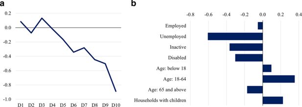
Change in the disposable income (left) and share of at risk of poverty (right). (a) Equivalised disposable income by decile (deviation from baseline; %). (b) At risk of poverty (excluding unreported wages) (deviation from baseline; % points). Note: Own calculations. The income cut points for deciles and median income used for estimation of at risk of poverty threshold (60% of median) are based on the baseline scenario for 2018. The figures show the results of the CGE-EUROMOD model.

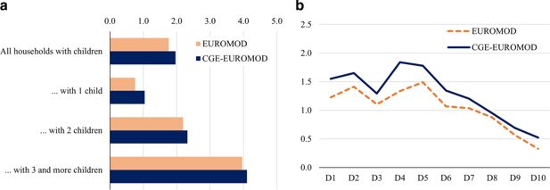
Changes in equivalised disposable income (deviation from baseline; %). (a) By number of children. (b) By decile of equivalised disposable income. Note: Own calculations. Income cut points for deciles are based on the baseline scenario for 2021 and are constant across models.
Tables
Aggregate statistics on evaluated unreported wage payments in 2018
| The share of employees with unreported wage; % | The ratio of unreported wage to legal gross wage for employees with non-zero unreported payments; % | |
|---|---|---|
| Total | 19.2 | 23.3 |
| 1st quintile (based on legal gross wage) | 42.3 | 44.5 |
| 2nd quintile | 37.5 | 23.8 |
| 3rd quintile | 15.3 | 17.6 |
| 4th quintile | 4.4 | 14.9 |
| 5th quintile | 1.5 | 15.9 |
-
Note: Own calculations.
Changes in selected indicators and selected industries in response to the financial services shock simulation (deviation from baseline in 2018; %)
| Variable | Total | Financial services | Auxiliary financial services | Wood production | Construction |
|---|---|---|---|---|---|
| Real output | –0.44 | –13.25 | –3.06 | 0.13 | –0.23 |
| Nominal gross wage | –0.33 | –4.13 | –1.26 | –0.20 | –0.28 |
| Nominal gross wage (high-skilled) | –0.38 | –5.11 | –1.31 | –0.16 | –0.29 |
| Nominal gross wage (medium-skilled) | –0.35 | –3.51 | –0.97 | –0.21 | –0.29 |
| Nominal gross wage (low-skilled) | –0.25 | –1.60 | –0.47 | –0.21 | –0.25 |
| Employment | –0.13 | –12.21 | –2.72 | 0.15 | –0.19 |
-
Note: Own calculations.
Family benefit by number of dependent children ( euro per month)
| Year | Family with 1 dependent child | Family with 2 dependent children | Family with 3 dependent children | Family with 4 dependent children |
|---|---|---|---|---|
| 2021 | 11.38 | 44.14 | 122.90 | 229.8 |
| 2022 | 25.00 | 100.00 | 225.00 | 400.00 |
-
Note: Own calculations. We assume that in 2021 the sequential number of children corresponds to the actual number of dependent children in a family.
Multinomial logistic regression
| (1) | (2) | (3) | (4) | (5) | (6) | (7) | (8) | |
|---|---|---|---|---|---|---|---|---|
| Men | Men | Men | Men | Women | Women | Women | Women | |
| Variables | Low-skilled | Medium-skilled | Unemployed | Inactive | Low-skilled | Medium-skilled | Unemployed | Inactive |
| Secondary education | –1.612*** | –1.669*** | –2.251*** | –2.339*** | –1.098* | –0.207 | –2.155*** | –2.619*** |
| Tertiary education | –4.405*** | –4.264*** | –4.769*** | –4.967*** | –4.268*** | –2.471*** | –4.603*** | –5.142*** |
| Age | –0.068*** | –0.068*** | –0.124*** | –0.266*** | –0.049*** | –0.057*** | –0.105*** | –0.212*** |
| Age2 | 0.001*** | 0.001*** | 0.002*** | 0.003*** | 0.001*** | 0.001*** | 0.001*** | 0.002*** |
| Cities other than Riga | 0.441*** | 0.410*** | 0.472*** | 0.489*** | 0.097** | 0.028 | 0.456*** | 0.141*** |
| Thinly populated area | 0.636*** | 0.506*** | 0.772*** | 0.855*** | –0.070* | –0.194*** | 0.405*** | 0.320*** |
| Married | –0.262*** | –0.153*** | –0.701*** | –0.831*** | –0.142*** | –0.078* | 0.006 | 0.241*** |
| Household non-employment income, per household member, in logs | 0.028*** | 0.034*** | 0.028** | 0.059*** | –0.007 | –0.010 | –0.032*** | 0.003 |
| Earnings of other household members, per household member, in logs | –0.034*** | –0.066*** | –0.171*** | –0.158*** | –0.019*** | –0.003 | –0.126*** | –0.065*** |
| Number of children under 3 years of age | –0.112* | –0.067 | –0.788*** | –0.656*** | –0.015 | –0.199** | 1.087*** | 1.107*** |
| Disabled | 0.917*** | 0.170 | 3.153*** | 4.945*** | 0.839*** | 0.749** | 3.313*** | 4.879*** |
| Paying mortgage | –0.512*** | –0.560*** | –0.869*** | –0.819*** | –0.478*** | –0.458*** | –0.614*** | –0.478*** |
| Constant | 3.363*** | 3.514*** | 5.567*** | 7.843*** | 3.264*** | 1.945** | 5.276*** | 7.517*** |
| Observations | 33’055 | 33’055 | 33’055 | 33’055 | 36’220 | 36’220 | 36’220 | 36’220 |
| Years | Yes | Yes | Yes | Yes | Yes | Yes | Yes | Yes |
-
*** p<0.01, ** p<0.05, * p<0.1.
-
Note: Own calculations. Data used is EU-SILC 2011-EU-SILC 2019, Latvia. High-skilled is base outcome of the multinomial logistic regression.
Heckman selection model
| (1) | (2) | (3) | (4) | |
|---|---|---|---|---|
| Men | Men | Women | Women | |
| Variables | Relative wage in logs | Selection model | Relative wage in logs | Selection model |
| Secondary education | 0.348*** | 0.387*** | 0.443*** | 0.495*** |
| Tertiary education | 0.521*** | 0.669*** | 0.566*** | 0.806*** |
| Medium-skilled | 0.173*** | –0.036 | 0.124*** | –0.021 |
| High-skilled | 0.355*** | 0.241*** | 0.289*** | 0.314*** |
| Age | 0.041*** | 0.003 | 0.014*** | 0.027*** |
| Age2 (*1000) | –0.525*** | –0.227** | –0.177*** | –0.417*** |
| Cities other than Riga | –0.088*** | –0.051 | –0.159*** | –0.079*** |
| Thinly populated area | –0.068*** | –0.227*** | –0.148*** | –0.198*** |
| Married | 0.089*** | 0.227*** | 0.008 | –0.217*** |
| Household non-employment income, per household member, in logs | – | –0.010 | – | –0.010* |
| Earnings of other household members, per household member, in logs | – | 0.101*** | – | 0.062*** |
| Paying mortgage | – | 0.472*** | – | 0.134*** |
| Number of children under 3 years of age | – | 0.253*** | – | –0.911*** |
| Disabled | – | –1.003*** | – | –1.044*** |
| Number of months spent in full-time work | 0.085*** | – | 0.098*** | – |
| Number of months spent in part-time work | 0.015*** | – | 0.034*** | – |
| Constant | –2.223*** | 0.500** | –2.033*** | –0.024 |
| atanh() | –0.411*** | – | –0.474*** | – |
| ln() | –0.486*** | – | –0.392*** | – |
| Observations | 24’477 | 24’477 | 28’384 | 28’384 |
| Years | Yes | Yes | Yes | Yes |
-
*** p<0.01, ** p<0.05, * p<0.1.
-
Note: Own calculations. Data used is EU-SILC 2011–EU-SILC 2019, Latvia. Dependent variable in wage equation is employment income relative to the industry average (in logs).
Changes in selected macroeconomic, fiscal and income distribution variables in response to two scenarios (deviation from baseline; %).
| Variable | Scenario 1: Shock to financial services | Scenario 2: Changing family benefits |
|---|---|---|
| Macroeconomic variables | ||
| Real GDP | –0.44 | 0.28 |
| Real private consumption | –0.17 | 0.81 |
| Real investments | –0.42 | 0.26 |
| Real exports | –0.70 | –0.13 |
| Real imports | –0.25 | 0.30 |
| GDP deflator | –0.22 | 0.15 |
| Consumption deflator | –0.16 | 0.11 |
| Export deflator | –0.12 | 0.08 |
| Import deflator | 0.00 | 0.00 |
| Unemployment (percentage points) | 0.09 | –0.07 |
| Employment | –0.13 | 0.10 |
| Employment (high-skilled) | –0.17 | 0.09 |
| Employment (medium-skilled) | –0.20 | 0.13 |
| Employment (low-skilled) | –0.04 | 0.10 |
| Gross real wage | –0.17 | 0.09 |
| Gross nominal wage | –0.33 | 0.20 |
| Gross nominal wage (high-skilled) | –0.38 | 0.19 |
| Gross nominal wage (medium-skilled) | –0.35 | 0.21 |
| Gross nominal wage (low-skilled) | –0.25 | 0.20 |
| Gross nominal reported wage | –0.44 | 0.26 |
| Fiscal variables | ||
| Budget balance (percentage points to GDP) | –0.28 | –0.06 |
| Budget expenditures | 0.10 | 0.65 |
| Social expenditures | 0.31 | 2.58 |
| Old-age pensions | –0.02 | 0.02 |
| Disability pensions | 0.00 | 0.00 |
| Sickness benefits | 0.00 | 0.00 |
| Unemployment benefits | 5.72 | 0.07 |
| Family-related benefits | 0.00 | 14.39 |
| Other benefits | 0.04 | –0.15 |
| Budget revenues | –0.65 | 0.50 |
| Social security contribution revenues | –0.64 | 0.30 |
| Personal income tax revenues | –0.97 | 0.37 |
| Value added tax revenues | –0.54 | 0.96 |
| Excise tax revenues | –0.39 | 0.55 |
| Income distribution (EUROMOD-CGE) | ||
| Gini coefficient (equivalised total disposable income) | –0.25 | –0.44 |
| Gini coefficient (equivalised reported disposable income) | –0.32 | –0.48 |
| S80/S20 (equivalised total disposable income) | –0.01 | –0.65 |
| S80/S20 (equivalised reported disposable income) | –0.11 | –0.85 |
-
Notes: Own calculations. Baseline for Scenario 1 is the year 2018, for Scenario 2 - the year 2021.
Data and code availability
The codes for separate EUROMOD model are publicly available. The EUROMOD software and the model (coded policies) can be downloaded from the website of the European Commission: https://euromod-web.jrc.ec.europa.eu/download-euromod. EUROMOD input EU-SILC-based microdata can be requested from the EUROSTAT following a specific procedure described on the same website.
CGE and CGE-EUROMOD code is proprietary to Bank of Latvia, with executable also not available. Latvia's Supply and Use tables for 2015 are publicly available at the web page of the Central Statistical Bureau of Latvia: https://stat.gov.lv/lv/statistikas-temas/valsts-ekonomika/ikp-gada/cits/2408-piedavajuma-izlietojuma-un-ielaides-izlaides.


