Economy-Wide Effect of Fiscal Drag in Ethiopia
- Adnan Abdulaziz Shahir: University of Bologna, Italy
- Francesco Figari: University of Eastern Piedmont, Italy
- Solomon Tsehay Feleke: Addis Ababa University, Ethiopia
Abstract
This study evaluates the economy-wide effect of fiscal drag in Ethiopia, focusing on household consumption expenditure and income. Drawing on a prior study that used the ETMOD tax-benefit micro-simulation model and assessed the effect of fiscal drag on income distribution and work incentives, this study uses a static CGE model. The simulation introduces a 9.1 percent increase in the average income tax rate due to the failure of the tax system to update the monetary tax parameters for inflation. The study allows for unemployment in agricultural labor, and four critical conclusions are drawn from the empirical investigation. First, fiscal drag reduces consumption expenditure by urban non-poor households but fosters consumption outlays by the urban poor, rural poor, and rural non-poor households due to a fall in saving that outweighs the negative impact due to the increase in the income tax rate for the three household categories. Second, an inflation-driven increase in income tax rates decreases disposable income for urban households while increasing the disposable income of rural counterparts who face higher prices of their factors of production. Third, fiscal drag slightly increases economic growth, household consumption, and export but reduces imports. Fourth, the upsurge in revenue from direct tax due to fiscal drag more than offsets the fall in government revenue from indirect taxes mainly due to the reduction of consumption of the urban non-poor households.
1. Introduction
Over the past decade, Ethiopia has experienced high inflation rates, with yearly rates ranging from 6.6 to 24.1 percent (IMF, 2020). The growth of money supply and a shock in agricultural production determine the short-run change in inflation, while exchange rates and world prices dictate the inflation trend in the long run (Simpasa et al., 2011; Durevall and Sjö, 2012). Denbel et al. (2016) found that inflation in Ethiopia is a monetary phenomenon negatively affected by economic growth. Barro (2013) multi-country study showed that a 10 percent increase in inflation results in a 0.2–0.3 percent drop in real per capita GDP growth.
Inflation also distorts the tax system and worsens the tax burden on taxpayers unless the tax schedule is adequately indexed for price changes regularly (Aaron, 1976; Tanzi, 1980). In a progressive tax system with fixed monetary tax parameters, with the failure to implement a comprehensive and full-scale adjustment on tax schedules, exemptions, and deductions for inflation the so called fiscal drag emerges: a rise in nominal income that pushes previously exempted individuals into the tax band, increases the marginal tax rate for taxpayers, lowers real disposable income, and encourages tax evasion and informality (Tanzi, 1980). Despite its relevance, the effects of fiscal drag on income distributional and macroeconomy have not been well researched in Africa. This paper aims to fill this gap in the empirical public economics literature.
The next section reviews some of the studies that contributed to the current understanding of the macroeconomic effects of changes in discretionary tax policies. However, the microeconomic implications of a rise in the income tax rate owing to fiscal drag are often overlooked. Against this backdrop, our study aims to investigate the economy-wide effect of fiscal drag in Ethiopia, focusing on household income and consumption dimensions. The study discusses why the effects of fiscal drag differ across heterogeneous household groups. It implements a bottom-up micro-macro link-up approach to introduce a shock in a CGE model by feeding a change in the average effective income tax rate caused by fiscal drag originating from an application of ETMOD, the static Ethiopian tax-benefit microsimulation model developed within the SOUTHMOD project (Shahir and Figari, 2022).
More specifically, this study contributes to the literature on the effects of fiscal drag in developing economies. To the best of our knowledge, it is the first to specifically explore the macroeconomic effect of fiscal drag in Africa integrating a micro-macro model. The study relies on the Ethiopian 2015/16 Social Account Matrix (SAM) built by Planning and Development Commission (PDC) in collaboration with the authors of this study. We used the recent SAM to ensure consistency of the findings with the country’s contemporary economic characteristics.
The remainder of the paper is organized as follows. Section 2 reviews the main literature on the effects of fiscal drag based on microsimulation approaches and the macroeconomic effects of income tax reforms. Section 3 presents the key characteristics of SAM, and the features of income tax in Ethiopia are discussed in Section 4. Section 5 describes the micro-micro link-up technique implemented to bring shocks into the macro model. Section 6 presents the CGE model, the macroeconomic closure rules, and relevant equations for this study. Section 7 delves deeper into the empirical findings, concentrating on the impact of fiscal drag on major economic indicators, focusing on household consumption expenditure and income. Section 8 concludes the paper. In addition, the appendix presents a detailed overview of the Ethiopian 2015/16 SAM and info on the CGE model used in the study.
2. Literature review
We review two strands of the literature. First, we discuss studies that applied microsimulation methods to assess the impact of fiscal drag on income distribution and work incentives. Second, we delve in-depth into studies that examined the macroeconomic effects of income tax reforms.
Most of the studies to date on fiscal drag apply a tax-benefit microsimulation model and are limited to the industrialized world. Such research seeks to uncover the effects of inflation-triggered bracket creep and benefit erosion on the progressivity of tax policy, tax burden, work incentives, poverty, and inequality. Immervoll (2000) showed that, under a progressive tax system, a shrink in the initial value of tax parameters due to inflation produces distortion for all taxpayers, especially for individuals previously exempted from tax liability. Empirical studies indicate that fiscal drag raises the average tax rate (Immervoll, 2000; Zhu, 2015). Immervoll (2005) and Levy et al. (2010) found that fiscal drag reduces the progressivity of income tax. The study by Immervoll (2006) showed that unless tax schedules, exemptions, and deductions are adjusted adequately for inflation, fiscal drag decreases work incentives. In addition, Paulus et al. (2020) demonstrated that indexation results in a higher reduction in poverty and inequality compared to discretionary policy reforms.
The pioneer research on fiscal drag in Africa was conducted by Abedian and Biggs (1995). They computed effective average tax rates from the year 1972 to 1994 using five groups of hypothetical taxpayers with annual earnings of 10,000, 20,000, 40,000, 60,000, and 90,000 South African Rands measured in 1988 constant prices. Their finding shows that discretionary changes of tax parameters with monetary value did not offset the effects of inflation on the tax burden throughout the period under consideration. Shahir and Figari (2024) investigated the impact of fiscal drag on income distribution and work incentives in Ethiopia, Mozambique, South Africa, Tanzania, Uganda, and Zambia. The authors applied a tax-benefit microsimulation approach. The study revealed that fiscal drag shrinks work incentives in all countries while reducing the progressivity of personal income taxes, except in Mozambique, where the tax system exhibits a regressive structure.
Fiscal drag is conventionally considered as an automatic stabilizer that cools the overheating economy during an inflationary period (Packer, 1965); however, such assertion ignores the counterproductive effects of a higher effective tax rate increasing the cost of production on the supply side (Immervoll, 2006). To the best of our knowledge, no study investigated the economy-wide effect of fiscal drag in Africa, particularly in Ethiopia. We attempt to analyze how a fiscal drag-driven increase in the income tax rate affects the economy, emphasizing the outcome on household income and consumption.
Focusing on studies that employ a Computable General Equilibrium (CGE) model to investigate the effects of change in the income tax rate on the macroeconomy, most of them show that the economic impact of a change in income tax depends on the labor market structure. Dernburg (1974) argued that an increase in personal income tax reduces disposable income in countries with weaker labor unions. In the unionized labor market, workers retaliate and demand an increased wage rate for a corresponding increase in income tax. Such measures could keep the disposable income from falling despite the increase in tax liability. Jackson et al. (1972) and Pitchford and Turnovsky (1976) supported this wage-tax spiral argument.
However, previous studies based on CGE models for the developed economies demonstrated that the macroeconomic impact of an income tax reform is far from convergence. Diamond and Viard (2008) revealed that a tax cut in the U.S. boosts long-run output by jeopardizing the fiscal deficit. Conversely, according to Bovenberg et al. (2000), tax reduction in the higher tax band increased labor supply in the formal market but failed to raise employment, particularly for unskilled labor. Böhringer et al. (2005) also found that an income tax reform in Germany had a small role in alleviating unemployment in a highly unionized labor market.
Studies in developing countries reveal a negative relationship between the increase in income tax rate and household income and consumption. Amir et al. (2013) studied the effects of changes in personal and corporate income taxes in Indonesia. Lowering the marginal tax rate on personal income boosts household consumption and income. Chiripanhura and Chifamba (2015) revealed that reducing the income tax rate in Namibia improves consumption and disposable income, especially for urban households. Llambi et al. (2016) found that raising personal income tax reduces private consumption in Uruguay under a flexible government saving scenario. According to Bhattarai et al. (2019), a three-percentage point reduction in the corporate income tax rate in Vietnam fosters consumption and disposable in the top quintiles and negatively affects poor households who get transfers from the government.
In Ethiopia, the economy-wide effects of income tax reform are rarely explored. Nikus (2021) is a pioneer and the only CGE-based study on the subject matter. The author applied a recursive dynamic general equilibrium model to investigate the macroeconomic effects of tax reforms in Ethiopia. The study showed that a 30% reduction in income tax increased household consumption and income. However, the study reported simulation results under full employment assumption in the factor market despite a massive unemployment problem in the country, particularly in the agricultural sector.
3. Social accounting matrix
A Social Accounting Matrix (SAM) is a comprehensive and economy-wide database that records all economic interactions between agents in a specific territory within a definite period (Mainar-Causapé et al., 2018). A SAM is an extension of the Input-Output table through incorporating institutional accounts such as households, enterprises, government, and the rest of the world. A SAM is a single-entry accounting; the income of an account is recorded in rows while expenditure is shown in columns (Reinert and Roland-Hoist, 1987). Nevertheless, it resembles the double-entry accounting procedure, where the sums of the corresponding rows and columns are equal (Pyatt, 1988). Each cell in a SAM implies the payment from the account of a column to the respective account of a row. The accounts determine the dimension of the square matrix, where rows and columns are identically tabulated.
According to King (1985), a SAM offers dual benefits to the users. First, it shows the snapshots of the economic structure of a country or a region in a specific period. It demonstrates key economic balances, such as fiscal surplus and current account balance, and provides options to researchers to compile Gross Domestic Product (GDP) in production, income, and expenditure approaches. Second, a SAM is the main input to explore the effect of policy interventions either using multiplier analysis or a Computable General Equilibrium (CGE) model.
SAM highlights the interaction and the circular flow of income receipts and payments among the different elements of the economy such as activity, goods and services, factors, and institutions. The circular flow diagram, presented in Figure 1, captures the entire real transactions between actors and institutions. A payment made by an agent becomes another agent’s income. Productive activity purchases labor, land, and capital from the factor market and intermediate inputs from the commodity market to produce goods and services. The activity can hire factors from the domestic market, perhaps also from the rest of the world. The commodity market buys the domestically produced items and supplements them with imports to make the total supply. It exports goods and services to the rest of the world and generates hard currency for the economy. Institutions, which own the factors of production, use the remuneration paid by domestic activity and the rest of the world to purchase goods and services for final demand from the commodity market, pay taxes, and make inter-institutional transfers. It also makes direct payment to productive activity in case there is an item for home consumption.
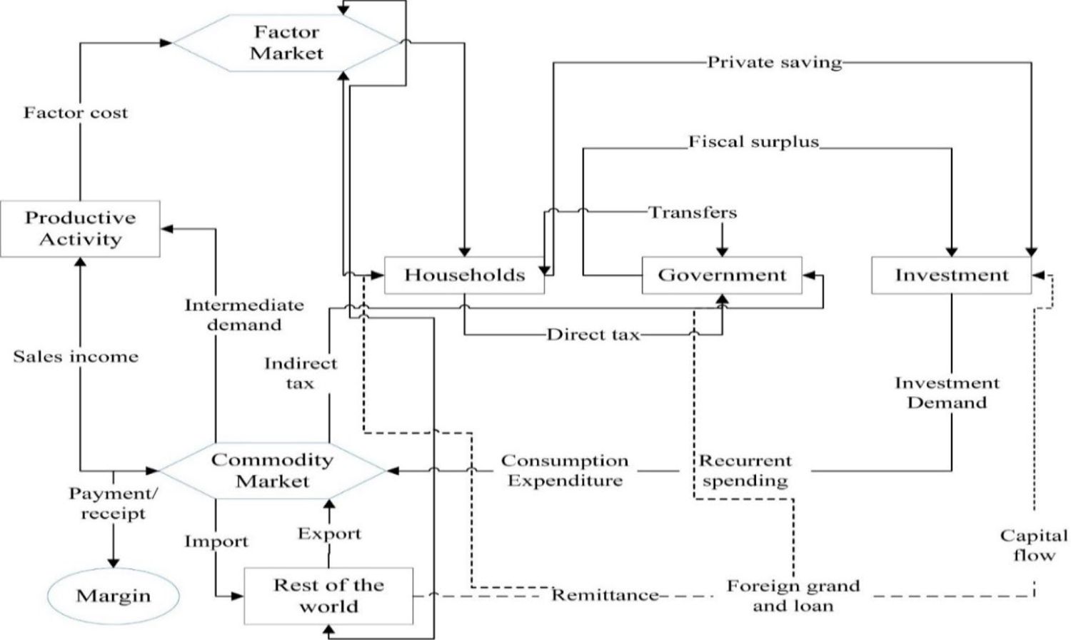
Circular flow diagram. Source: Own elaboration.
4. Income tax in Ethiopia
Income tax holds a considerable stake in the total tax revenue in Ethiopia. Figure 2 presents the share of income tax over total tax revenue and the percentage of tax from employment and business profit over total income tax. This figure shows that direct taxes accounted for 37 percent of total tax receipts in 2015. The significance of this tax has grown over time, reaching 46 percent in 2020. Concerning indirect taxes, a larger share of government tax revenue comes from VAT on domestic and imported goods. Domestic indirect taxes vary, but import taxes fell considerably between 2015 and 2019 (Shahir and Figari, 2022).

Trend of direct tax in Ethiopia. Source: Own computation.
The income tax in Ethiopia includes employment income tax, rental income tax, business profits, withholding income tax on imports, agriculture income tax, interest income tax, capital gains tax, and other income tax. However, employment income tax and business profit tax account for most income tax revenue, and they are indeed the subjects of this research. Figure 2 shows that the share of employment income and business profit taxes over aggregate income tax varies with a slight growing trend between 87 and 90 percent from 2015 to 2020. The tax base includes any payments or gains in cash or in-kind received by an individual from employment, ongoing payment from former employment or otherwise, or advance payments from future jobs. In contrast, business profit tax refers to income tax on profits of both sole proprietorships and corporations. Shahir and Figari (2022) reported that employment income tax contributes around 16 percent, while business profit tax owes around 21 percent of the total tax revenue in the 2020 fiscal year.
Overall, the tax revenue mobilization is at a low level in Ethiopia. Between 2013 and 2019, the maximum tax revenue to GDP ratio was 8.8 (World Bank, 2021). In Ethiopia, low revenue collection is a result of extensive illegal financial outflows, sluggish economic structural reform, and generous tax incentives provided to attract foreign direct investment (Kibret and Mamuye, 2016). A weak tax revenue mobilization performance is also clearly exhibited in the 2015/16 SAM. Figure 3, depicted using the 2015/16 micro-SAM, reports the share of income tax revenue (blue bars), the share of income (grey bars) and the average effective income tax rates (orange dots) by household types. The Figure shows these indicators for the household categories included in the 2015/16 SAM: urban poor, urban non-poor, rural poor, and rural non-poor households. The national absolute poverty line was employed to identify poor and non-poor households. Poor households in rural and urban regions contribute relatively little to income tax revenues and pay extremely low income tax rates. The tax burden significantly falls on non-poor households, especially those living in the urban parts of the country. Urban non-poor households account for 83 percent of income tax revenue with an average income tax rate of around 10%. The rural non-poor households provide 16 percent of income tax revenue, with an average income tax rate of around 2%. However, non-poor households in urban areas earn a smaller percentage of total household income than their rural counterparts.
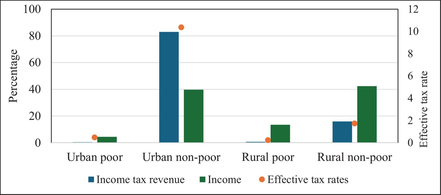
Income tax revenue, income, and effective tax rates by household types. Source: Own computation.
5. Micro–macro link
The application of a CGE model is often confined to examine the economic impacts of changes in macroeconomic policies. The model does not allow the detection of the distributional impact of the shock at the household level. In contrast, micro-simulation models provide individual and household-specific effects of policy changes. These models are commonly used to examine the impact of reforms on inequality and poverty, but they do not capture the general equilibrium effects. However, macro-oriented policy reforms have micro-level implications. For instance, a decline in unemployment due to a macro shock certainly reduces the number of poor households. Micro-level policy adjustments, such as increasing cash transfers, also have a ripple effect across the economy due to changes in saving and labor supply (Cockburn et al., 2014).
The literature identifies five main techniques to link macro and micro models to explore the effects of macro-level policy change on households or quantify a macroeconomic impact of a shock with micro-foundations: representative household approach, fully integrated approach, top-down approach, bottom-up approach, and iterative approach (Bourguignon and Bussolo, 2013).
The representative household approach involves clustering households in the CGE model into groups. The household clusters are commonly formed using education, gender, location, and income. It is a pioneering method applied by research to look at the micro effects of macro shocks. Researchers apply this technique to investigate the impacts of macro policy on poverty and inequality by plugging the change estimated in the CGE model into a survey database with household-level income and consumption variables. Lofgren et al. (2003) demonstrated the application of representative households for distributional analysis. However, the representative household approach assumes that households grouped under the same category have identical behavior. The main objection to the approach relates to its limitation in measuring the deviation within the representative household. Adelman and Robinson (1978) and Derviş et al. (1982) used lognormal distribution to account for heterogeneity within the cluster. While Decaluwe et al. (1999) modeled the within-cluster distribution using beta distribution.
The fully integrated approach can incorporate entire households from the survey into a CGE model. The technique does not require linking a shock from the macro model with a standalone microsimulation model but produces directly poverty and inequality indicators. This approach enables modelling the observed heterogeneity among households. However, it demands technical skills and programming capacity to reconcile the household survey with other databases and run the model without errors. Savard (2003) and Bourguignon and Savard (2008) discussed that the approach does not capture discrete choice features in the labor market. The fully integrated method was initially applied by Decaluwe et al. (1999).
The top-down approach entails feeding the output from a CGE model into a microsimulation model. For example, a change in prices or wage rates from the CGE model fed into the micro model. The top-down method is simpler to implement compared to the fully integrated technique. It also addresses some limitations of the representative household approach by enabling computation of the distributional effects of macro policies for both between and within household groups. This method does not consider the feedback effect from micro to macro models; however, a change in household behavior due to the macro shock might have a second-round impact on macro variables. Ravallion and Lokshin (2008) and Chen and Ravallion (2004) are among the studies that applied a top-down approach.
The bottom-up approach takes information from the micro to macro model. This approach is useful to simulate a macro shock with a micro base like a reform in tax and benefit policies. Changes in elasticities, tax rates, or labor supply are usually used as linkage variables. Analogous to a top-down approach, the bottom-up method disregards the micro effects of the feedback of the CGE model. Boeters et al. (2006) applied a bottom-up approach to analyze the effects of counterfactual reforms on social assistance benefits in Germany, while Filho et al. (2010) used the method to examine the effects of proposed tax reform on fiscal balance, employment, and growth effects.
The iterative approach extends a bidirectional shock from macro to micro models and vice versa. The technique iteratively combines top-down and bottom-up approaches. Price or wage rates supply information in the top-down part, while elasticities, tax rates, or labor supply links feedback in bottom-up components; the linkage variables should be exogenous in the recipient model. The iteration process continues by updating the linkage factor till the point of convergence between the two models. Up on convergence, the iterative approach will be consistent with a fully integrated model (Bourguignon and Bussolo, 2013). The iterative method was employed in literature by Bayar et al. (2021), Mussard and Savard (2010), and Savard (2010). The fundamental drawback of this approach is that convergency may not be maintained after several iteractions (Savard, 2003).
Micro-macro models are rarely applied in tax-benefit analyses; instead, they are better utilized for trade policy analysis (Peichl, 2009). Our study uses a bottom-up approach to feed a shock simulated with a tax-benefit microsimulation model into a CGE model. As shown in Figure 4, the average income tax rate is the linkage variable that supplies the feedback from ETMOD to a CGE model, described in Section 6. ETMOD is a tax-benefit microsimulation model for Ethiopia based on EUROMOD platform with underpinning micro data computed based on the most recent three rounds of the Ethiopian Socioeconomic Survey (Shahir and Figari, 2022).

Bottom-up approach. Source: Adapted from Bourguignon and Bussolo (2013).
Considering a cumulated 55 percent of inflation over the period cover in this study (2014-2018), Shahir and Figari (2024) indicate that fiscal drag in Ethiopia increases the average income tax by 9.1 percent. We used this change in the effective income tax rate to implement an exogenous shock in the CGE model.
We used the change in the effective average income tax rate to supply information from ETMOD to the CGE model. The VAT does not effectively pass a shock into CGE since it is a flat rate in Ethiopia. Hence, inflation does not raise indirect taxes revenue in real terms. In addition, a change in labor supply is commonly used in the literature to take feedback from the micro to macro models. However, tax policies have an insignificant role in triggering a change in labor supply behavior in Sub-Saharan countries (McKay et al., 2019). Therefore, labor cannot be a proper linkage factor for our research. Changes in the average effective tax rates have been already used to link micro and maccro models employing a bottom-up approach (see Feltenstein et al. (2013) and Zhang (2017).
The micro-macro link-up technique applied in this study adheres to the literature regarding conditions for convergency. Peichl (2016) stated that convergence between the two models is achieved when the changes in the linkage variables are (close to) zero. Given the interest of this study, the deviation in factor prices from the CGE model would be an ideal linkage factor for the top-down part if we decided to adopt the iterative approach. But Table A2 in the Appendix indicates a fall in wage rates for semi-skilled and skilled workers due to fiscal drag close to zero. These two labor categories account for 73 percent of income for the urban non-poor household ( Table A4 in the Appendix), which contributes for 83 percent of income tax revenue (Figure 3). In this regard, feeding the difference in wage rate into the microsimulation under the iterative macro-micro link-up framework would not produce a different result relative to the bottom-up approach used in the study. The fall in wages rate (0.07 percent) is trivial to cancel out the initial price shock in ETMOD (55 percent).
6. Computable general equilibrium (CGE) model
A CGE model is a standard tool for empirical policy analysis, particularly in developed countries. A CGE model is mostly applicable for single country analysis but can be employed for studies varying from the global level to households in a small village of a country. A CGE model is a collection of simultaneous equations, most of which are non-linear. The equations represent the behavior of economic agents; some of these equations capture the production and consumption decisions derived from the respective first-order neo-classical profit and utility maximization conditions. In addition, the set of equations hold certain constraints or closure rules that must be satisfied to get an optimal solution. Parts of the variables in the equation are endogenous; the rest is not determined within the model. A CGE model presupposes goods and factors markets are competitive (Bergman, 1982; Lofgren et al., 2002).
A SAM and elasticities are the primary inputs for a CGE model. A SAM, offering the benchmark state of the economy, is a database to calibrate the parameters of a model to reproduce the base estimate. The CGE model embodies blocks of equations that resemble the standard structure of the SAM. The additional data for the CGE model are the elasticities of substitution for the CES production functions, the elasticities of substitution for imports and exports relative to domestic commodities, the income elasticities of demand for the linear expenditure system (Table A6), and the Frisch elasticities (marginal utility of income), in Table A7. The values attributed to elasticities can be determined based on econometric estimations or adopted from previous literature from countries with similar socio-economic characteristics.
We have employed the STAGE model to assess the macroeconomic effect of fiscal drag. STAGE is a GAMS-based single country general equilibrium model that requires a country specific SAM for calibration. GAMS code and model technical documents are composed by McDonald (2015). The STAGE family models belong to the group of CGE models built upon neoclassical theories. It conforms with the price relationships and accounting conventions in the System of National Accounts (SNA) and the System of Environmental-Economic Accounts (SEEA). The model includes the following 11 blocks of equations: trade, commodity price, numéraire, production, factor, household, enterprise, government, capital, foreign institutions, and market clearing block. The profit and utility optimality conditions for the economic agents in the model are constrained by technology and factor supply.
The model is defined by the behavioral relationship, which is either linear or non-linear, that dictates how agents respond to an exogenous shock. The non-linear behavioral relationship governs consumption, production, and trade decisions. Households consume goods and services to satisfy utility represented by the Stone Gary utility function which is preferred because it allows for subsistence consumption expenditures, which is a highly reasonable assumption given Ethiopia’s high poverty rate. Consumers choose bundles from a set of composite products. Composite products are formed by aggregating imported and domestic products using the Constant Elasticity of Substitution (CES). It implies that domestic and imported products are imperfect substitutes. The optimal mix between domestic and imported products is determined by the relative price of the domestic and imported products (Armington, 1969). This hypothesis is known as the 'Armington insight.' Due to the lower share of Ethiopian products in the international commodity market, the model assumes the country as a price taker on imported items.
6.1 Macroeconomic closure
The exchange rate is fixed while the external balance is flexible in the model. This closure condition is ideal for Ethiopia where the exchange rate is not entirely governed by market forces. Further, the world price for exported and imported commodities are fixed in line with a small country assumption. Regarding the capital closure, investment-driven saving closure is selected where investment is fixed but saving rates change to maintain saving-investment in equilibrium. For government account closure, the study maintains fixed tax rates and government consumption expenditure. While government saving is endogenous. The CPI is chosen as a numeraire, indicating that transfers and wages are in real terms. The numeraire is used as a base because the model is defined only with relative prices, and it has a homogenous degree zero in terms of price. Finally, al. primary factors except agricultural labor are fully employed and perfectly mobile. Therefore, the study endogenizes unemployment in agriculture.
6.2 Relevant equations
Two important equations specified in the STAGE version of the CGE model allow monitoring changes in key variables of the analysis: household consumption expenditure and income. Equation 1 represents household consumption expenditure (); household allocates income () net of direct tax, saving, and inter-household transfers () for consumption outlays. While Equation 2 shows the numbers of variables in the saving rate () equation. It comprises a fixed ratio of saving to disposable income in the base solution (), absolute change in the base rates ), a multiplicative savings rate scaling factor for households (), a multiplicative saving rate scaling factor for both households and enterprises (), an additive adjustment factors for households (), an additive adjustment factor for both households and enterprises (), and partial change in savings rates (). and have an initial value of 1 while , , , and hold 0 initial value (McDonald, 2015).
7. Results
This section presents the effect of fiscal drag on the Ethiopian economy. We discuss the effect of the simulated shock on household consumption and income, macroeconomy, and fiscal indicators with a focus on assessing how fiscal drag alters consumption and income by household categories.
7.1 Impact of fiscal drag on household consumption and income
An increase in the income tax rate has a morning-after effect of decreasing disposable income for all households. The effect size varies by household type and is proportional to the direct tax rate on household income. As Figure 3 shows, urban non-poor households contribute the largest share of income tax revenue with a 10.37 tax rate. Hence, this household type encounters the biggest drop in disposable income due to fiscal drag. On the other hand, poor rural households account for a lower share of income tax revenue. Consequently, the rise in income tax rate has minimal effect on its disposable income.
According to Equation 1, household consumption expenditure is defined as household’s after-tax income less savings and transfers to other households. Thus, the fall in disposable income would cause, in principle, a reduction in household consumption expenditures on most commodities. According to the simulation results, consumption expenditure by all household categories increases on commodities with negative income elasticities. However, the study found a mixed effect on the household consumption expenditures on commodities with positive income elasticity. The findings show that a fall in disposable income may not necessarily reduce household consumption expenditure. As indicated in Table 1, the 9.1 percent increase in the income tax rate due to fiscal drag reduces household consumption expenditure only for urban non-poor household while it increases for urban poor, rural poor, and rural non-poor households. This divergent effect ascribed to relative change in direct tax rate and the saving rate.
Percentage change in household consumption and income.
| Household types | Household consumption | Household income |
|---|---|---|
| Urban poor | 1.31 | -0.06 |
| Urban non-poor | -0.75 | -0.08 |
| Rural poor | 0.70 | 0.16 |
| Rural non-poor | 0.33 | 0.07 |
-
Source: Own computation.
Due to data limitation, the 2015/16 SAM doesn’t account for inter-household transfers. Therefore, the change in household consumption expenditure, in Equation 1, is ultimately determined by respective changes in the income tax rate and saving. Keeping everything else constant, the decline in disposable income due the increase in direct tax rate could reduce consumption expenditure by all household categories. Nevertheless, the deviation saving rate could revert the cumulative effect of fiscal drag on consumption expenditure.
The adopted investment-driven saving closure requires adjusting household savings to maintain equilibrium between saving and investment. Therefore, in this study, the only variable allowed to change from Equation 2 is the savings rate scaling factor, which is used to increase the saving rate in the base solution. This condition enables the system to generate sufficient savings to fund the exogenous investment. Aggregate savings consist of household savings, government savings, and foreign savings. As demonstrated in section 7.3, government savings increased significantly due to fiscal drag. Consequently, the household saving rate decreased by 1.74 percent to maintain a balance between saving and investment.
The reduction in saving rate has caused a divergent effect of fiscal drag on consumption expenditure by different groups of households. The 2015/16 SAM indicates that urban non-poor household, which contributes 83 percent of direct tax, has a lower saving rate. Thus, the effect of an increase in the income tax rate on consumption surpasses the impact due to a decrease in the saving rate. On the contrary, the remaining three household groups possess a very lower direct tax rate. Hence, the effect of a fall in saving rate on consumption spending outweighs the impact due to the increase in the income tax rate.
Table 1 also shows how a 9.1 percent increase in the income tax rate affects household income, given the fact that earnings from factors of production account for a more significant part of household income. The shock has caused a drop in income for urban households but resulted in a rise in income for rural households. On the one hand, households in rural areas are exceptionally less exposed to income tax, and the fiscal drag effect is only trivial. On the other hand, the price of a factor of production owned in a greater quantity by these household groups increased because of fiscal drag. Generally, the study found that two variables jointly determine whether the household gains or losses due to fiscal drag: the percentage of urban non-poor consumption of major consumption items and change in the price of factors the household owned in large quantity.
Table 2 illustrates the proportion of consumption by urban non-poor households and the change in household consumption and production among the top ten consumption items. The share of consumption by urban non-poor households is compiled based on the 2015/16 SAM. The result reveals that fiscal drag significantly reduces the consumption expenditure by urban non-poor households on major commodities, while it boosts consumption by the remaining categories of households. The simulation has a mixed effect on the production of selected items.
Share of consumption and changes in household consumption and production.
| Item | Share of consumption by urban non-poor | Household consumption expenditure | Production | |||
|---|---|---|---|---|---|---|
| Urban Poor | Urban non-poor | Rural poor | Rural non-poor | |||
| Grain | 20.65 | 0.16 | - 0.09 | 0.38 | 0.18 | 0.14 |
| Livestock | 28.92 | 1.67 | -0.95 | 0.87 | 0.40 | 0.10 |
| Hotel | 41.58 | 1.86 | -1.01 | 0.63 | 0.30 | -0.13 |
| Forest | 18.53 | 2.06 | -1.13 | 1.26 | 0.59 | 0.37 |
| Agro-processing | 25.39 | 0.16 | -0.09 | 0.38 | 0.18 | 0.14 |
| Other service | 60.88 | 1.87 | -1.00 | 0.64 | 0.31 | -0.14 |
| Real estate | 63.86 | 1.88 | -0.99 | 0.65 | 0.32 | -0.34 |
| Transport | 52.93 | 1.87 | -1.00 | 0.64 | 0.31 | 0.13 |
| Alcohol | 53.91 | 0.17 | -0.09 | 0.39 | 0.19 | 0.06 |
| Textile | 27.11 | 0.92 | -0.50 | 0.88 | 0.42 | 0.31 |
-
Source: Own computation.
The direction of change in production correlates with the proportion of urban non-poor’s consumption on major commodities. When the non-poor urban is the primary customer, its consumption changes alter the production of related goods or services. Hence, the decrease in urban non-poor consumption disincentives the production of the same product, freeing up factors to the production of other items. In this respect, fiscal drag lowers the production of hotels, other services, and real estate products, predominantly consumed by urban non-poor households. Table 2 also indicates an increasing production of grain, livestock, forest, agro-processing, and textile production, where urban non-poor has lower consumption share. Transportation and alcohol commodities are widely consumed by urban non-poor. With an increase in income tax rate, exceptionally their productions also increase. Despite the fall in consumption by urban non-poor household, the surge in transport production is due to it being a valuable export item, while an increase in alcohol consumption by other household groups exceeds the drop in consumption by non-poor urban households.
Table 3 shows the percentage change in factor demand to produce major consumption items. Fiscal drag has resulted in a drop in demand for semi-skilled labor, skilled labor, and other capital in sectors where production has declined, namely hotels, other services, and real estate activities. On the contrary, fiscal drag has fostered the demand for semi-skilled labor, skilled labor, and other capital in sectors where production has increased, specifically grain, livestock, forest, agro-processing, transport, alcohol, and textile activities. Eventually, the drop in demand for the above factors exceeds the increase in demand, resulting in a fall in factor price, as shown in Table A2 in the Appendix. Moreover, fiscal drag increased the demand and prices for factors of production mainly utilized in agricultural sectors. However, the price for agricultural labor remained fixed due to the labor market closure rule adopted in this study. An increase in demand for factors hired in the agricultural sector is due to consumption boost by the urban poor, rural poor, and rural non-poor households and increased intermediate demand by manufacturing activities like grain and agro-processing.
Percentage change in factor demand by selected activities.
| Items | Agricultural labor | Non-irrigated land | Irrigated land | Agricultural capital | Semi-skilled labor | Skilled labor | Other capital |
|---|---|---|---|---|---|---|---|
| Grain | 0.17 | 0.19 | 0.22 | ||||
| Livestock | 0.20 | 0.04 | |||||
| Hotel | -0.11 | -0.10 | -0.07 | ||||
| Forest | 0.40 | 0.23 | |||||
| Agro-processing | 0.16 | 0.18 | 0.21 | ||||
| Other services | -0.15 | -0.13 | -0.11 | ||||
| Real estate | -0.38 | -0.37 | -0.34 | ||||
| Transport | 0.12 | 0.14 | 0.16 | ||||
| Alcohol | 0.03 | 0.04 | 0.07 | ||||
| Textile | 0.28 | 0.30 | 0.33 |
-
Source: Own computation.
The change in household income, illustrated in Table 1, is also dictated by the variation in the price of factors the household owned in large quantities. Households exhibit an increase/ decrease in income if the demand for a factorthey own in larger quantities increases/ decreases. Households whose income is primarily derived from a factor with increased factor price are better off. The results show that rural households gained income while urban households lost due to the shock. Table A4 in the Appendix reports that urban households get the lion’s share of their income from semi-skilled labor, skilled labor, and other capital, whose prices have decreased. Contrary, rural households get a large part of their income from agricultural labor, non-irrigated land, irrigated land, and agricultural capital. The prices for these factors have increased because of fiscal drag (Table A2 in the Appendix), apart from the fixed agricultural labor price due to the closure rule we adopted. According to Table 1, the poor rural household achieved the highest increase in income; because of a production boost in the primary sector and a reduction in unemployment for agricultural labor (Table A5 in the Appendix).
7.2 Macroeconomic impact
Table 4 illustrates the macroeconomic effect of an average income tax rate increase when the tax system is not indexed to cope with inflation. The simulation results indicate that real GDP and domestic production increased by 0.04 percent. Household consumption has also increased by 0.03 percent in real terms; the rise in consumption expenditure by other households offset the fall in urban non-poor households. As a result of the shock, exports increased by 0.03 percent, while imports declined by 0.05 percent. The decline in consumption expenditure by urban non-poor households and the resulting price drop are the main reasons for a minor export increase and a drop in imports. Our findings reveal that fiscal drag has a minimal macroeconomic impact in Ethiopia, which can be explained by the country’s low-income tax rate (see Figure 3).
Macroeconomic effects of an increase in the income tax rate.
| Real GDP | 0.04 |
|---|---|
| Real domestic production | 0.04 |
| Real household consumption | 0.03 |
| Real domestic final demand | 0.02 |
| Real import | -0.05 |
| Real export | 0.03 |
| Real intermediate input | 0.05 |
-
Source: Own computation.
7.3 Fiscal impact
An increase in government revenue from direct tax is the immediate effect of the fiscal drag. As shown in Table 5, the direct tax revenue has increased by 9.05 percent. This refers to the tax burden placed on taxpayers so long as the monetary tax parameters are not adjusted for inflation. The decline in import volume has led to reduced tax revenue from import tariffs. Similarly, the fall in consumer expenditure by urban non-poor households, who often consume items subject to indirect taxes, lowered sales tax, VAT, and excise tax. Ultimately, fiscal drag has a positive net effect on government revenue; government income has increased by 2.89 percent.
Effects of an increase in the income tax rate on government income and expenditure.
| Direct tax | 9.05 |
|---|---|
| Import tax | -0.02 |
| Sales tax | -0.11 |
| VAT | -0.38 |
| Excise tax | -0.04 |
| Government income | 2.89 |
| Government expenditure | -0.08 |
| Government savings | 6.91 |
-
Source: Own computation.
8. Conclusions
This study has evaluated the economy-wide effect of fiscal drag in Ethiopia, focusing on household consumption expenditure and income. The study applied a STAGE variant of the CGE model developed by McDonald (2015). We introduced a 9.1 percentage increase in the average income tax rate for the failure of the tax system to index the monetary tax parameters for inflation, drawn from a tax-benefit microsimulation exercise conducted by Shahir and Figari (2024) on the impact of fiscal drag on income distribution and work incentives. The CGE model is calibrated using the 2015/16 SAM. Further, the study used the factor market closure rule that fixes the supply of all factors apart from the agricultural labor.
Our findings suggest that taxpayers who earn a higher share of their income through formal employment suffer the most from fiscal drag. Inflation-induced increase in income tax rate reduces consumption expenditure of urban non-poor but fosters consumption outlays of urban poor, rural poor, and rural non-poor households. The impact on consumption resulting from a decrease in the saving rate outweighs the initial increase in the income tax rate for all household categories except urban non-poor. However, fiscal drag reduces income for urban poor and urban non-poor households. The increase in the income tax rate reduced factor demand for semi-skilled labor, skilled labor, and other capital, which are primarily used to produce commodities predominantly consumed by urban non-poor. Such factors constitute the largest share of income for urban poor and non-poor households.
According to the study, fiscal drag slightly favors economic growth in Ethiopia. The simulation result indicates a slight increase in domestic production, household consumption, and intermediate inputs. Similarly, it increases export but shrinks imports given a fixed foreign exchange closure rule. The fall in import volume and consumption expenditure by urban non-poor have reduced revenue from indirect taxes. Moreover, fiscal drag boosts the government revenue from tax sources. The upsurge in revenue from direct tax sufficiently dominates the fall in government income from indirect taxes. However, the increase in tax revenue is almost completely faced by urban non-poor households who encounter a fall in disposable income and consumption. Moreover, Shahir and Figari (2024) showed that fiscal drag implies detrimental distributive impacts in Ethiopia by reducing the progressivity of the income tax and the financial work incentive to increase income by either working more hours or finding a job with better pay.
These findings suggest the importance of introducing a statutory adjustment to monetary tax policy parameters. Indexing the nominal tax parameters eliminates the inflation-driven tax burden on urban non-poor households. In addition, an inflationary adjustment fo tax thresholds will incentivize taxpayers to stay in formal employment. Similarly, lowering the tax burden might encourage businesses which do not pay taxes to formalize their activity.
Appendix A
A.1. Overview of the Ethiopian 2015/16 micro-SAM
The activity and commodity accounts follow International Standard Industrial Classification (ISIC Rev 3.1). Hence, these two accounts contain the following classifications: Agriculture, forestry, fishing, manufacturing, electricity, gas, water, construction, wholesale and retail trade, hotels and restaurants, transportation and communication, financial intermediation, real estate, public administration and defense, education, health and social work, other social and personal service activities, and activities of private households. Specifically, agriculture includes crop and livestock sectors. Our Classification Follows ISIC Rev 3.1, except for grouping the mining and quarrying activities under non-metallic categories of the manufacturing sector.
Table A1 presents the detailed elements of major accounts of the SAM. Accordingly, the SAM has 81 activities and 83 commodities; fertilizer and gas are the only items fully imported for domestic use. The 2005/06 SAM is the first comprehensive economic database for Ethiopia (EDRI, 2009). The factor accounts in the 2015/16 SAM include agricultural labor, non-irrigated land, irrigated land, skilled labor, semi-skilled labor, other agricultural capital, and capital. The SAM also has four households: urban poor, urban non-poor, rural poor, and rural non-poor. Similarly, the tax account contains direct tax, sales tax, VAT, excise tax, and import tax.
The 2015/16 SAM for Ethiopia used administrative data and multiple surveys covering different dimensions of economic activities in agricultural and manufacturing sectors. It also used the 2015/16 annual GDP estimate and the 2015/16 Supply and Use Table (SUT), generated by PDC, to fill the data gap in the service activities as well as to align the preliminary SAM estimates with national account statistics.
A.2. Balancing SAM
Before balancing, the micro-SAM values, especially components directly estimated from surveys, have been aligned to official macroeconomic statistics. Micro-SAM characterizes the economy at the detail level of disaggregation, while macro-SAM depicts the aggregate macroeconomic variables. The row and column balance in macro-SAM represents the balance in national account statistics. Further, the micro-SAM is compute enrolling the top-down approach. This technique maintains coherence with official economic statistics and avoids huge discrepancies from the initial stage. The construction of micro-SAM involves three stages. First, the prior macro-SAM is computed using data from the national economic account, balance of payments statistics, and government financial statistics. The prior macro-SAM provides control totals for various economic flows. Second, an imbalanced micro-SAM is created by disaggregating the prior macro-SAM with extensive details, particularly on activities, commodities, factors, taxes, and representative households using survey data, except figures in the service sectors derived from the supply-use table. The imbalance between row and column minimized to the lowest possible point employing a manual procedure. Eventually, the inconsistency between the row and column sum reached below three percent. Third, the miss-match between the sum of the corresponding row and column in the micro-SAM is reconciled using the General Algebraic Modelling System (GAMS) based SAM balancing program, Cross-Entropy methods. The program encompasses ten mandatory steps, but the user can modify only the first, second, eighth, and tenth steps.
A.3. The macro-SAM
The balanced final macro-SAM for Ethiopia for the year 2015/16 (Table A1) is produced by aggregating the balanced micro-SAM. The aggregation overlook heterogeneity across producing unit, commodities, and households. Nevertheless, this doesn’t affect the simulation results that entirely relied on micro-SAM. The balanced final macro-SAM demonstrates the aggregate circular flow numerically and allows the compilation of indicators like GDP and macroeconomic balances. The micro-SAM has undergone the necessary transformations and adaptations to achieve coherence with the corresponding official stats.
The activity and commodity accounts comprise the agriculture, service, and industry categories. This arrangement allows simple exposition of the pattern of category-wise demand for intermediate input and factors by productive activity and the mix of domestic supply and imports in the commodity market. Accordingly, the macro-SAM shows that industrial sectors possessing the highest intermediate input to output ratio (0.68) offer the lowest value-added. The remuneration for labor constitutes the highest share from value-added in all three categories. Moreover, the industrial sector contains the highest ratio of imports from the aggregate supply (0.23) at a basic price. Moreover, 71 percent of indirect tax is collected from the use of industrial commodities.
Macro-SAM also demonstrates the allocation of varieties of factor income among urban and rural households. Urban and rural households receive 44 percent and 56 percent of the factor income, respectively. A large portion of direct tax is disproportionately contributed by urban households, owning 83 percent of the aggregate. Further, industrial goods attract the highest share of consumption expenditure from the two household types. Urban and rural households have 22 percent and 26 percent saving rates, respectively. Export earning is dominated by foreign currency inflow by supplying services to the international market, specifically the transport service, followed by agriculture.
A.4. CGE Model description
Figure A1 shows the production technology for output at the activity level. The model includes three stages of the production process for domestic production. At the first level, CES technologies combine aggregate intermediate consumption and aggregate value addition. The ratio of aggregate intermediate input and factors varies with the relative price of intermediate consumption and value added. At the second level, intermediate inputs are aggregated using Leontief technology, and different primary factors are aggregated using CES. The ratio of intermediate input demand is in fixed proportions to aggregate intermediates, whereas the proportion of demand for components of value-added varies with relative prices. At the third level, it involves aggregating different kinds of factors of production like skilled labor semi-skilled labor, and unskilled labor using CES. Primary factors (land, labor, and capital) are combined and supplied for aggregation at the second level (McDonald, 2015).
The STAGE version of the CGE model allows activity to engag e in the production of multiple products. CES technology is employed in this study to combine different products from the activity. The optimal ratio of the products of an activity is determined by the relative prices. Likewise, domestic production is allocated between domestic demand and export using the Constant Elasticity of Transformation (CET). The optimal allocation of domestic production between domestic and export demand relies on relative price of exported and domestically supplied commodities. It indicates product differentiation and an imperfect transformation between domestic use and export demand.
Balanced Macro SAM for the year 2015/16.
| Activity | Commodity | Margin | Factor | Household | Tax | Govt | Kapital | World | Total | |||||||||||||
|---|---|---|---|---|---|---|---|---|---|---|---|---|---|---|---|---|---|---|---|---|---|---|
| Agri | Indus | Service | Agri | Indus | Service | Labor | Land | Capital | Urban | Rural | direct | Indirect | ||||||||||
| Activity | Agri | 649 | 649 | |||||||||||||||||||
| Indus | 1,124 | 1,124 | ||||||||||||||||||||
| Service | 806 | 806 | ||||||||||||||||||||
| Commodity | Agri | 48 | 320 | 65 | 89 | 199 | 10 | 48 | 779 | |||||||||||||
| Indus | 46 | 365 | 114 | 201 | 342 | 0 | 531 | 13 | 1,613 | |||||||||||||
| service | 4 | 77 | 125 | 172 | 169 | 138 | 166 | 0 | 67 | 917 | ||||||||||||
| Margin | 98 | 70 | 4 | 172 | ||||||||||||||||||
| Factor | Labor | 357 | 221 | 333 | 911 | |||||||||||||||||
| Land | 20 | 20 | ||||||||||||||||||||
| Capital | 174 | 142 | 168 | 483 | ||||||||||||||||||
| Household | Urban | 468 | 0 | 150 | 1 | 66 | 686 | |||||||||||||||
| Rural | 443 | 20 | 333 | 2 | 70 | 868 | ||||||||||||||||
| Tax | Direct | 60 | 12 | 72 | ||||||||||||||||||
| Indirect | 82 | 33 | 115 | |||||||||||||||||||
| Govt | 45 | 72 | 115 | 30 | 262 | |||||||||||||||||
| Kapital | 123 | 176 | 92 | 150 | 541 | |||||||||||||||||
| World | 32 | 338 | 74 | 445 | ||||||||||||||||||
| Total | 649 | 1,124 | 806 | 779 | 1,613 | 917 | 172 | 911 | 20 | 483 | 686 | 868 | 72 | 115 | 262 | 541 | 445 | |||||
-
Source: Own computation.

Production technology. Source: Own elaboration.
Percentage change in Factor prices.
| Non-irrigated land | Irrigated land | Agricultural capital | Semi-skilled labor | Skilled labor | Other capital |
|---|---|---|---|---|---|
| 0.27 | 1.83 | 0.20 | -0.07 | -0.07 | -0.12 |
-
Source: Model simulation results.
Percentage distribution of household income by factor types.
| Factor types | Urban poor | Urban nonpoor | Rural poor | Rural nonpoor |
|---|---|---|---|---|
| Agricultural labor | 2.37 | 0.15 | 94.54 | 28.12 |
| Non-irrigated land | 0.16 | 0.04 | 5.23 | 1.08 |
| Irrigated land | 0.23 | 0.45 | ||
| Agricultural capital | 1.07 | 0.06 | 28.84 | |
| Semi-skilled labor | 41.39 | 47.22 | ||
| Skilled labor | 55.01 | 25.43 | 14.83 | |
| Other capital | 27.10 | 26.68 |
-
Source: Model simulation results.
Percentage change in unemployment.
| Unemployment in agricultural labor |
|---|
| -8.24 |
-
Source: Model simulation results.
List of main Account of the 2015/16 SAM for Ethiopia.
| Activities | Commodities | Factors | Households | Taxes | ||||
|---|---|---|---|---|---|---|---|---|
|
|
|
|
|
|
|
|
|
-
Source: Own compilation.
Income elasticities for Ethiopia.
| Commodities | Urban poor household | Urban non-poor household | Rural poor household | Rural non-poor household |
|---|---|---|---|---|
| Teff | 1.14 | 1.14 | 1.08 | 1.08 |
| Barley | 0.33 | 0.33 | 0.06 | 0.06 |
| Wheat | 0.41 | 0.41 | 0.42 | 0.42 |
| Maize | 0.58 | 0.58 | 0.62 | 0.62 |
| Sorghum | - 0.81 | - 0.81 | 1.00 | 1.00 |
| Finger millet | - 0.81 | -0.81 | 1.00 | 1.00 |
| Oats | 0.33 | 0.33 | 0.64 | 0.64 |
| Rice | 0.13 | 0.13 | 0.64 | 0.64 |
| Horse beans | 0.87 | 0.87 | 1.13 | 1.13 |
| Peas | 0.87 | 0.87 | 1.13 | 1.13 |
| Haricot beans | 0.87 | 0.87 | 1.13 | 1.13 |
| Lentils | 0.87 | 0.87 | 1.13 | 1.13 |
| Vetch | 0.87 | 0.87 | 1.13 | 1.13 |
| Other pulse | 0.87 | 0.87 | 1.13 | 1.13 |
| Neug | 2.10 | 2.10 | 0.96 | 0.96 |
| Linseed | 2.10 | 2.10 | 0.96 | 0.96 |
| Groundnuts | 2.10 | 2.10 | 0.96 | 0.96 |
| Sesame | 2.10 | 2.10 | 0.96 | 0.96 |
| Other cereals | -6.70 | -6.70 | 2.30 | 2.30 |
| Other spices | 0.67 | 0.67 | 0.30 | 0.30 |
| Other oilseeds | 2.10 | 2.10 | 0.96 | 0.96 |
| Peppers | 0.67 | 0.67 | 0.30 | 0.30 |
| Other vegetable | 0.87 | 0.87 | 0.95 | 0.95 |
| Onion | 0.87 | 0.87 | 0.95 | 0.95 |
| Potato and sweat potato | 0.59 | 0.59 | 0.18 | 0.18 |
| Garlic | 0.67 | 0.67 | 0.30 | 0.30 |
| Taro godere | 0.59 | 0.59 | 0.18 | 0.18 |
| Other root crop | 0.59 | 0.59 | 0.18 | 0.18 |
| Bananas | 0.87 | 0.87 | 0.95 | 0.95 |
| Other fruits | 0.87 | 0.87 | 0.95 | 0.95 |
| Chat | 0.85 | 0.85 | 1.39 | 1.39 |
| Coffee | 0.85 | 0.85 | 1.39 | 1.39 |
| Cotton | 0.85 | 0.85 | 1.39 | 1.39 |
| Hops | 0.85 | 0.85 | 1.39 | 1.39 |
| Sugarcane | 0.85 | 0.85 | 1.39 | 1.39 |
| Enset | - 0.39 | -0.39 | 2.12 | 2.12 |
| Flower | 1.50 | 1.50 | 1.72 | 1.72 |
| Livestock | 1.23 | 1.23 | 1.22 | 1.22 |
| Forest | 1.50 | 1.50 | 1.72 | 1.72 |
| Fishing | 0.12 | 0.12 | 0.52 | 0.52 |
| Preserve | 0.12 | 0.12 | 0.52 | 0.52 |
| Vegetable oil | 0.90 | 0.90 | 0.83 | 0.83 |
| Dairy | 0.12 | 0.12 | 0.52 | 0.52 |
| Grain | 0.12 | 0.12 | 0.52 | 0.52 |
| Bakery | 0.12 | 0.12 | 0.52 | 0.52 |
| Sugar | 0.96 | 0.96 | 0.16 | 0.16 |
| Argo-processing | 0.12 | 0.12 | 0.52 | 0.52 |
| Animal feed | 0.12 | 0.12 | 0.52 | 0.52 |
| Alcohol | 0.12 | 0.12 | 0.52 | 0.52 |
| Soft drinks | 0.12 | 0.12 | 0.52 | 0.52 |
| Tobacco | 1.50 | 1.50 | 1.72 | 1.72 |
| Textile | 0.67 | 0.67 | 1.19 | 1.19 |
| Apparel | 0.67 | 0.67 | 1.19 | 1.19 |
| Leather | 0.67 | 0.67 | 1.19 | 1.19 |
| Wood | 1.50 | 1.50 | 1.72 | 1.72 |
| Papier | 1.50 | 1.50 | 1.72 | 1.72 |
| 1.50 | 1.50 | 1.72 | 1.72 | |
| Chemicals | 1.50 | 1.50 | 1.72 | 1.72 |
| Fertilizer | 1.50 | 1.50 | 1.72 | 1.72 |
| Ink | 1.50 | 1.50 | 1.72 | 1.72 |
| Soap detergent | 1.50 | 1.50 | 1.72 | 1.72 |
| Pharmaceutical | 1.50 | 1.50 | 1.72 | 1.72 |
| Rubber | 1.50 | 1.50 | 1.72 | 1.72 |
| Non-metal | 1.50 | 1.50 | 1.72 | 1.72 |
| Metal | 1.50 | 1.50 | 1.72 | 1.72 |
| Electrical | 1.50 | 1.50 | 1.72 | 1.72 |
| Machinery | 1.50 | 1.50 | 1.72 | 1.72 |
| Furniture | 1.50 | 1.50 | 1.72 | 1.72 |
| Gas | 1.50 | 1.50 | 1.72 | 1.72 |
| Construction | 1.50 | 1.50 | 1.72 | 1.72 |
| Water | 1.35 | 1.35 | 0.86 | 0.86 |
| Transport | 1.35 | 1.35 | 0.86 | 0.86 |
| Trade | 1.35 | 1.35 | 0.86 | 0.86 |
| Real | 1.35 | 1.35 | 0.86 | 0.86 |
| Public | 1.35 | 1.35 | 0.86 | 0.86 |
| Private | 1.35 | 1.35 | 0.86 | 0.86 |
| Other service | 1.35 | 1.35 | 0.86 | 0.86 |
| Hotel | 1.35 | 1.35 | 0.86 | 0.86 |
| Health | 1.35 | 1.35 | 0.86 | 0.86 |
| Entertainment | 1.35 | 1.35 | 0.86 | 0.86 |
| Electricity | 1.35 | 1.35 | 0.86 | 0.86 |
| Education | 1.35 | 1.35 | 0.86 | 0.86 |
| Banking | 1.35 | 1.35 | 0.86 | 0.86 |
-
Source: Own compilation based on Hertel (1997) and Tafere et al. (2010).
Frisch elasticity
| Urban poor household | Urban non-poor Household | Rural poor household | Rural non-poor household |
|---|---|---|---|
| -5.85 | -5.85 | -5.85 | -5.85 |
-
Source: Own compilation based on Hertel (1997).
References
- 1
-
2
Fiscal Drag in South Africa: 1972–1994South African Journal of Economics 63:184–191.https://doi.org/10.1111/j.1813-6982.1995.tb01240.x
-
3
Income Distribution Policy in Developing Countries: A Case Study of KoreaStanford, Calif: Stanford University Press.
-
4
The impact of the Indonesian income tax reform: A CGE analysisEconomic Modelling 31:492–501.https://doi.org/10.1016/j.econmod.2012.12.018
-
5
A theory of demand for products distinguished by place of productionIMF Economic Review 16:159–178.https://doi.org/10.2307/3866403
- 6
-
7
Ministry of Economic and Finance WP 2021-14Ministry of Economic and Finance WP 2021-14.
-
8
A system of computable general equilibrium models for a small open economyMathematical Modelling 3:421–435.https://doi.org/10.1016/0270-0255(82)90040-9
-
9
Impacts of Direct and Indirect Tax Reforms in Vietnam: A CGE AnalysisEconomies 7:50.https://doi.org/10.3390/economies7020050
-
10
Reforming Social Welfare in Germany: An Applied General Equilibrium AnalysisGerman Economic Review 7:363–388.https://doi.org/10.1111/j.1468-0475.2006.00124.x
-
11
Taxation and unemployment: an applied general equilibrium approachEconomic Modelling 22:81–108.https://doi.org/10.1016/j.econmod.2004.05.002
-
12
The Impact of Macroeconomic Policies on Poverty and Income Distribution: Macro-Micro Evaluation Techniques and ToolsA CGE integrated multi-household model with segmented labor markets and unemployment, The Impact of Macroeconomic Policies on Poverty and Income Distribution: Macro-Micro Evaluation Techniques and Tools, Houndmills, England: Palgrave-Macmillan.
-
13
Handbook of Computable General Equilibrium Modeling1283–1437, Income distribution in computable general equilibrium modeling, Handbook of Computable General Equilibrium Modeling, Elsevier B.V, p, 10.1016/B978-0-444-59568-3.00021-3.
-
14
Tax reform and the Dutch labor market: an applied general equilibrium approachJournal of Public Economics 78:193–214.https://doi.org/10.1016/S0047-2727(99)00116-4
-
15
Welfare impacts of China’s accession to the World Trade OrganizationThe World Bank Economic Review 18:29–57.https://doi.org/10.1093/wber/lhh031
-
16
The Impact of Namibia’s Income Tax ReformInternational Food Policy Research Institute (IFPRI.
-
17
Handbook of Microsimulation Modelling275–304, Macro-Micro models, Handbook of Microsimulation Modelling, Emerald Publishing Limited, p, 10.1108/S0573-855520140000293008.
-
18
CREFA Working Paper 99-20. Que´bec: Universite´ LavalCREFA Working Paper 99-20. Que´bec: Universite´ Laval.
-
19
Nairobi: African Economic Research ConsortiumNairobi: African Economic Research Consortium.
-
20
The relationship between inflation, money supply and economic growth in Ethiopia: Co integration and Causality AnalysisInternational Journal of Scientific and Research Publications 6:556–565.
-
21
The macroeconomic implications of wage retaliation against higher taxationStaff Papers 21:758–788.https://doi.org/10.2307/3866556
-
22
General Equilibrium Models for Development PolicyCambridge, U.K: Cambridge University Press.
- 23
- 24
- 25
- 26
-
27
Tax Reform, Income Distribution and Poverty in Brazil: an Applied General Equilibrium AnalysisInternational Journal of Microsimulation 3:114–117.https://doi.org/10.34196/ijm.00030
- 28
- 29
-
30
The impact of inflation on income tax and social insurance contributions in EuropeEUROMOD Working paper.
-
31
Falling up the stairs: the effects of “bracket creep” on household incomesReview of Income and Wealth 51:37–62.https://doi.org/10.1111/j.1475-4991.2005.00144.x
-
32
Fiscal Drag: An Automatic StabilizerResearch in Labor Economics 25:141–163.https://doi.org/10.1016/S0147-9121(06)25006-4
- 33
-
34
United Nations Development Programme EthiopiaUnited Nations Development Programme Ethiopia.
-
35
Social Accounting Matrix: Basis for Planning17–51, What Is a SAM, Social Accounting Matrix: Basis for Planning, Washington, D.C, The World Bank, p.
-
36
Simulating the impact of inflation on the progressivity of personal income tax in BrazilRevista Brasileira de Economia 64:405–422.https://doi.org/10.1590/S0034-71402010000400004
-
37
Assessing the Impacts of A Major Tax Reform: A CGE-microsimulation analysis for UruguayInternational Journal of Microsimulation 9:134–166.https://doi.org/10.34196/ijm.00131
-
38
A Standard Computable General Equilibrium (CGE) Model in GAMSA Standard Computable General Equilibrium (CGE) Model in GAMS, Vol, 5, Washington, D.C, International Food Policy Research Institute.
-
39
The Impact of Economic Policies on Poverty and Income Distribution: Evaluation Techniques and Tools325–337, Poverty and inequality analysis in a general equilibrium framework: the representative household approach, The Impact of Economic Policies on Poverty and Income Distribution: Evaluation Techniques and Tools, World Bank Publications, p.
-
40
Social Accounting Matrices: basic aspects and main steps for estimation. JRC Technical ReportsPublications Office of the European Union.
- 41
- 42
-
43
Macro/Micro Modelling and Gini Multi-Decomposition: An Application to the PhilippinesJournal of Income Distribution® 19:51–78.https://doi.org/10.25071/1874-6322.17482
-
44
Economy-wide impact of tax reform in Ethiopia: A recursive dynamic general equilibrium modelJournal of Accounting and Taxation 13:78–88.
-
45
Economic Significance of Fiscal DragFinancial Analysts Journal 21:127–133.https://doi.org/10.2469/faj.v21.n6.127
-
46
Indexing Out of Poverty? Fiscal Drag and Benefit Erosion in Cross‐National PerspectiveReview of Income and Wealth 66:311–333.https://doi.org/10.1111/roiw.12413
-
47
The Benefits and problems of linking micro and macro models — evidence from a flat tax analysisJournal of Applied Economics 12:301–329.https://doi.org/10.1016/S1514-0326(09)60017-9
-
48
Linking microsimulation and CGE modelsInternational Journal of Microsimulation 9:167–174.https://doi.org/10.34196/ijm.00132
-
49
Some effects of taxes on inflationThe Quarterly Journal of Economics 90:523–539.https://doi.org/10.2307/1885319
-
50
A SAM approach to modelingJournal of Policy Modeling 10:327–352.https://doi.org/10.1016/0161-8938(88)90026-9
-
51
The Impact of Macroeconomic Policies on Poverty and Income Distribution: Macro-Micro Evaluation Techniques and ToolsWinners and losers from trade reform in Morocco, The Impact of Macroeconomic Policies on Poverty and Income Distribution: Macro-Micro Evaluation Techniques and Tools, World Bank and Palgrave.
-
52
Applied Methods for Trade Policy Analysis: A Handbook94–121, Social Accounting Matrices, Applied Methods for Trade Policy Analysis: A Handbook, New York: Cambridge University Press, p, 10.1017/CBO9781139174824.006.
- 53
-
54
Scaling Up Infrastructure Spending in the Philippines: A CGE Top- Down Bottom-Up Microsimulation ApproachInternational Journal of Microsimulation 3:43–59.https://doi.org/10.34196/ijm.00024
- 55
-
56
The Effect of Fiscal Drag on Income Distribution and Work Incentives: A Microsimulation Analysis on Selected African Countries214–234, The Effect of Fiscal Drag on Income Distribution and Work Incentives: A Microsimulation Analysis on Selected African Countries, Vol, 92, South African Journal of Economics, p, 10.1111/saje.12375.
-
57
Inflation Dynamics in Selected East African Countries: Ethiopia, Kenya, Tanzania and UgandaAfDB Policy Brief.
-
58
Food Demand Elasticities in Ethiopia: Estimates Using Household Income Consumption Expenditure (HICE) Survey DataAddis Ababa: International Food Policy Research Institute.
-
59
Inflation and Personal Income Tax: An International Perspective Journal Macroeconomics (Vol. 3)Inflation and Personal Income Tax: An International Perspective Journal Macroeconomics (Vol. 3), Vol, 3, New York: Cambridge University Press, 10.1017/CBO9780511895661.
-
60
World Development Indicatorshttps://databank.worldbank.org/source/world-development-indicators, Accessed, 7 September 2021.
-
61
Solving a Partial Equilibrium Model in a CGE Framework: The Case of a Behavioural Microsimulation ModelInternational Journal of Microsimulation 10:27–58.https://doi.org/10.34196/ijm.00165
-
62
Bracket Creep Revisited With and Without R>G: Evidence From GermanyDeutsche Bundesbank.https://doi.org/10.2139/ssrn.2696932
Article and author information
Author details
Adnan Abdulaziz Shahir

Publication history
- Version of Record published: February 14, 2025 (version 1)
Copyright
© 2025, Colabella et al.
This article is distributed under the terms of the Creative Commons Attribution License, which permits unrestricted use and redistribution provided that the original author and source are credited.