Are Energy Bills Squeezing People’s Spending?
- Bank of Italy, DG for Economics, Statistics and Research - Financial Stability Directorate, Italy
- Bank of Italy, Climate Change and Sustainability Hub, Italy
Abstract
This paper presents an assessment of the energy price shocks that affected Italian households starting in mid-2021 and their impact on households’ financial vulnerability. First, we estimate the price elasticity of electricity and heating demand. Then, within the framework presented in Faiella and Lavecchia (2021b), we compute the variation between 2020 and 2022. Second, we study how those variations affected households’ financial vulnerability, based on an extension of the modeling strategy proposed by Faiella et al. (2022). Our results indicate that if energy price elasticity is not duly accounted for, financial vulnerability rises excessively following an energy price upsurge. However, when consumption rebalancing is taken into account, financial vulnerability remains rather low and in line with the supervisory data. While the risks for financial stability associated with energy shocks are therefore limited, this occurs at the expense of household consumption and welfare.
1. Introduction
At the beginning of 2021, energy prices rose on the heels of a combination of supply and demand factors.1 This structural increase was compounded by the Russian invasion of Ukraine on 24 February 2022, which resulted in an abrupt spike in energy prices on the global markets similar to that observed during the oil shocks of the 1970s.
Like other countries, Italy was hit by the increase in global energy prices, against a backdrop of this country’s heavy reliance on energy imports, which makes it especially vulnerable to energy price shocks. In fact, almost half of the electricity in 2021 and 60 per cent of all space heating in Italy were produced by burning natural gas, which, in the final months of 2021, was mostly imported (and mainly from Russia).2 In 2022, gas and electricity prices on the Italian markets skyrocketed, reflecting uncertainties about the continuity and security of the supply stream due to the increasing Russian threats to Ukraine in late 2021 and the ensuing all-out war.3 The energy shocks have had both direct and indirect effects on inflation: in the fourth quarter of 2022, the contribution to headline inflation was in the order of 60 per cent, and the contribution to core inflation between 20 and 50 per cent (Neri et al., 2023).
The abrupt price increases struck households unevenly, with those that spend a greater share of their budget on items that were more heavily impacted by the surging prices or with a higher average propensity to consume suffering the most (Curci et al., 2022; Faiella and Lavecchia, 2022; Guan et al., 2023). By eating away at households’ purchasing power, the price hikes ultimately reduce disposable income, hampering households’ ability to repay their debts. Depending on the amount of strain placed upon them, families could become more financially vulnerable and risks to financial stability could materialize.
This paper aims to analyse to what extent energy price hikes affect the financial vulnerability of Italian households. To this end, understanding how household energy markets work in Italy and which data are available to use is key to laying the ground for the analysis.
Retail gas and electricity markets both have a two-tier structure. In each segment, the price of the energy component is determined according to specific rules, set separately for each market.4 In greater detail, on the regulated market (Mercato di Maggior Tutela), the price of the energy component is set by the Italian Regulatory Authority for Energy, Networks and the Environment (Autorità di Regolazione per Energia Reti e Ambiente - ARERA) and updated quarterly.5 On the free market (Mercato Libero), the energy price is determined by market rules. In this market, contracts can have different price-setting mechanisms and lengths.
Given this complex structure, determining the impact of the inflation shock on households is not straightforward as we lack granular information, including on contractual length and the clauses for the price of the energy component paid by each household. Therefore, we have to rely on alternative data sources to fill in the void and use economy-wide energy price inflation measures. We apply the price increase indistinctly to all households; the exercise, therefore, establishes by construction an upper bound for their financial vulnerability. The results can also be interpreted as stemming from a stress test.
Bearing this in mind, we first determine price elasticities of electricity and heating for Italian households; this is necessary to understand how households cope with rising energy prices and, consequently, with a possible reduction in disposable income. To do so, we apply an updated version of the methodology proposed by Faiella and Lavecchia (2021b) to estimate the energy demand and price elasticities for Italian households. We use a quasi-panel approach as in Deaton (1985) to estimate price elasticities for 32 different household groups or strata using the Italian Household Budget Survey (HBS).
Therefore, when an electricity or heating price shock hits the economy, all the households adjust their consumption bundle accordingly. The adjustment is, however, stratum-specific (although we apply a stochastic adjustment at the household level) and reflects households’ characteristics and consumption preferences on the item shocked, which prevail at each level.
To measure the effects of the energy price shocks on households’ financial vulnerability, we first combine the consumption adjustment calculated above with microdata from the Bank of Italy’s 2020 Survey on Household Income and Wealth (SHIW) using the 32 strata as merging keys. This new dataset allows us to calculate an adjusted measure of households’ disposable income which reflects changes in consumption at the group level, induced by the energy price shocks. We hold that household disposable income diminishes proportionately to the increase in energy expenditure, if any. Households’ ability to repay their debt is affected by the reduced disposable income.
To dig further into the issue of financial vulnerability of households in Italy, we exploit to their full extent the microsimulation models developed at the Bank of Italy (Michelangeli and Pietrunti, 2014; Attinà et al., 2020; Faiella et al., 2022). Within these models, macroeconomic variables evolve reflecting macroeconomic data and projections.
In particular, in addition to the evolution of household income and debt, we extend the existing models by adding consumption dynamics.6
We run the simulations to check for financial vulnerability over the period 2020-22 and introduce the energy-induced shocks (via the adjusted income) to take into account the 2021-22 surge in energy-related inflation.
We compare the evolution of households’ vulnerability both in the absence and in the presence of behavioural responses/consumption adjustments,7 to respond to energy inflation shocks. In addition to a baseline case where there are no energy-induced price shocks, we apply such shocks under three different price scenarios, which refer to different price index evolution. In particular, we apply the energy price increase observed between 2020 and 2022 to all of the households recorded in: a) the regulated market tariffs (Mercato di Maggior Tutela); b) the electricity and natural gas components of the NIC Index (Istat’s consumer price index for the entire national community); and c) the weighted average unit cost of energy from Eurostat.
The change in the final price of electricity (natural gas) between the average in 2020 and the average in 2022 was 172 (92) per cent according to the first source (regulated market tariffs), 142 (109) per cent according to the second source (NIC index), and 46 (47) per cent according to Eurostat. In absolute terms, this equates to an increase between 0.11 (Eurostat) and 0.34 (NIC) €/kWh for electricity and between 10.9 (Eurostat) and 23.4 (NIC) €/Gj for natural gas, with regulated market tariffs being in-between.
If households do not re-adjust their consumption choices after the energy price upsurge (i.e. assuming perfect inelastic demand or quantity invariance), energy expenditure rises proportionately. This leads to a proportionate decrease in disposable income. At the same time, household financial vulnerability has barely changed in 2021, reflecting the contained growth in energy expenses. In 2022, instead, debt at risk increases across the three scenarios considered (to between 8.15 and 8.62 per cent, from 7.9 in the baseline), with the stronger increase occurring when the energy price upsurge is measured by the NIC Index. The contained increase in 2021 reflects the fact that energy price variations are subdued in the years 2020-2021, while they are more marked in 2021-2022. While at first sight, such increases may appear to be low, they are not: in fact, they mark up between 3 and 11 per cent increase from the baseline in 2022. This non-monotonic pattern in vulnerability, however, does not correlate well with actual financial evidence, according to which the new non-performing loan rate has not been spiking in the wake of the energy price shock and, even more important, it has decreased between 2021 and 2022 (Bank of Italy, 2023). To properly assess the evolution of financial vulnerability, it is therefore crucial to take into account households’ reactions and consumption rebalancing. We, therefore, extend our setup to include energy price elasticities.
In this setting, facing price increases, households decide to re-adjust their consumption so that disposable income drops only to a limited extent. Hence, financial vulnerability is barely affected. Throughout all the scenarios under consideration, the share of vulnerable households and the debt at risk appear to be very similar to those prevailing in the baseline scenario. This confirms that vulnerable households adjust their consumption expenditure in such a way as to maintain the level of disposable income as stable as possible so that it is also available for debt repayment.8 Looking at the heterogeneity results, we find very minor differences across scenarios. We can thus conclude that households’ vulnerability continues to be driven by macroeconomic variables other than energy price variations which in contrast have a limited impact. On the other hand, the muted impact could come at the cost of consumption reduction, thus lowering household welfare.
This paper innovates the existing literature along three dimensions. To the best of our knowledge, it is the first to take on board the effects of energy price increases via the correction in disposable income obtained by considering consumption elasticities in the analyses of households’ financial vulnerability. To do so, we extend the existing microsimulation models of financial vulnerability (Michelangeli and Pietrunti, 2014; Attinà et al., 2020; Faiella et al., 2022) to account for consumption dynamics. In other exercises, aimed at evaluating the effects of the recent price upsurge on Italian households along with the multi-pronged measures implemented by the Italian government to combat it, elasticities are set to be equal to zero, and no financial vulnerability analysis is performed (Curci et al., 2022; UPB, 2022; Istat, 2022).
Secondly, the paper evaluates the effects of energy price increases on households’ financial vulnerability, intertwining it with the evolution of macroeconomic variables, including mortgages and consumer credit to households.
While the topic of the analysis of households’ financial vulnerability partly aligns this work with that by Faiella et al. (2022), our setting allows us to have a richer interaction between the variables and relax one of the hypotheses assumed therein.
Thirdly, the paper merges several datasets. Such data stem from an updated series for energy-related products (for the period 1997 – 2022) that makes it possible to calculate energy-demand elasticities based on observations that refer to both pre-pandemic and pandemic conditions; at the same time, by using the 2020 wave of the SHIW, we can include the households’ debt variables available in the Italian survey, which also reflect the impact of the COVID-19 pandemic.
Finally, we would like to point out some caveats on the results obtained. First and foremost, the exercise is based on the assumption of partial equilibrium and does not include spillover effects; second, the time horizon we focus on is short, though this appears to be less of a concern at the current stage since the recent bout of energy-price inflation seems to be already dissipating. At the same time, in light of the magnitude of the price shock, structural breaks in elasticity can not be ruled out.
The structure of the paper is as follows. Section 2 offers an overview of the existing literature on the topics. Section 3 describes our data and methodologies for simulating the energy shock; we also provide a discussion of estimated energy price elasticities. Section 4 shows the set of models and data used to assess how the energy shock affects households’ financial vulnerability. The results of the study are shown in Section 5, which also includes some heterogeneity analyses. Section 6 concludes the paper and sets the future research agenda.
2. Literature review
This paper merges two different strands of literature.
The first is related to energy price elasticity; the second refers to microsimulation models. The latter strand can ideally be divided into three subset of papers: a) those dealing with methods to impute expenditures into an income data set; b) those connected to microsimulation models of households’ financial vulnerability; c) those, more recent, related to the uneven impact of rising energy prices on households’ standards of living.
Studies on the determinants of energy demand, especially electricity, are abundant both in temporal and spatial dimensions. From the first perspective, they date back several decades ago, kicking off with the seminal work of Houthakker (1951). Under the second viewpoint, there are, literally, hundreds of estimates of price elasticity, although most of them are based on US data. Espey and Espey (2004) report a meta-analysis of 36 papers, with more than 123 short-run and 96 long-run price elasticity estimates of residential electricity demand; in the short run, price elasticity ranges between -2.01 and -0.004 (mean: -0.35), while in the long run, elasticity ranges between -2.25 and -0.04 (mean: -0.85). Labandeira et al. (2017) carry out a meta-analysis for a dozen surveys on energy demand, again with mixed results, depending on the fuel considered and the time frame; as for electricity, elasticity is equal, on average, to -0.126 in the short run (-0.365 in the long run), while for natural gas it is equal to -0.180 in the short run (-0.684 in the long run). However, most of these studies are based, to different extents, on data from the United States, whose power sector is significantly different from Italy’s, along several dimensions, including in terms of market structure, prices and energy demand. In particular, the average American household consumes four times as much the amount of electricity as an average Italian household,9 with a significant contribution of electricity for space heating (one-third of all homes in the US appears to be fed by electricity for heating purposes, compared with an almost non-existing share in Italy).10
Estimates for energy demand price elasticity in the Italian case are just a few: Faiella (2011) finds that the effect of prices on the energy shares is negative for heating, while for electricity the effect is negative for the 1997-2004 period and positive for the 2005-2007 subsample. Bigerna (2012) observes that the price elasticity for electricity depends on the time of the day (due to the tariffs system in place up to 2016, which encourages off-peak use) and on the geographical zones, ranging between -0.03 and -0.10. Bardazzi and Pazienza (2019) observe that, concerning the age of the head of the households, electricity demand is hump-shaped, reaching a peak when the head of a household is 50 years old, while natural gas demand keeps increasing with age, as natural gas is the main component for heating in Italy, and the time spent at home increases. They also show that elasticities for electricity and natural gas (at the national level equal to -0.705 and -0.621, respectively) are higher in the Centre and the South. Finally, Favero and Grossi (2023) analyzes a sample of bills from Veneto, finding that the price elasticity for natural gas demand from residential customers is rather rigid (around - 0.5).
This paper also relates to the broad microsimulation literature. In this literature, the widespread methods to impute expenditures into an income data set are distinguished into two main categories: the so-called “explicit method”, based on the estimation of Engel curves, and the so-called “implicit method”, which uses statistical matching techniques. Decoster et al. (2020) cite the extensive literature on the topic and compares five different techniques.
In terms of financial vulnerability, our benchmark models are those developed by Attinà et al. (2020) and Michelangeli and Pietrunti (2014) at the Bank of Italy. Such models simulate the evolution of financial vulnerability of Italian households starting from SHIW data reconciled with macro-variables.
As for the impact of rising prices, including via carbon taxes, on households’ income and the uneven impact on their standards of living, there has been a blossoming of literature in recent years, also in relation to the recent inflation spike. We have no aim to cover it all and we will limit ourselves to papers more strictly related to the topic.
Faiella and Lavecchia (2021b) is, to the best of our knowledge, the only paper in Italy to put forward a methodology to estimate the demand and elasticity of energy-related items and to analyse the effects on consumption of a carbon tax. The authors combine the microdata of the Italian HBS with several external sources. They use a quasi-panel approach and estimate the demand elasticity via an autoregressive distributed lag (ARDL) model. They run several regressions applying many different estimation techniques and estimate the price elasticity for electricity and heating for 36 groups of Italian households in the short run (-0.44 and -0.54 on average for electricity and heating, respectively). In general, their results underscore that households’ price elasticity is greater in the long run and for transport fuels and electricity.
Faiella et al. (2022) apply the methodology developed in Faiella and Lavecchia (2021b) to determine the extent to which different levels of carbon taxes affect the financial vulnerability of households and firms. While taking into account the effects of energy price increases on the consumption bundle of households (and on the energy expenditure of firms), they run a static exercise and find that, within reasonable amounts of a carbon tax, the vulnerability of households and firms is only barely hit by energy-related shocks.
Curci et al. (2022) evaluate the sharp rise in prices registered in 2021-22 on the purchasing power of different types of Italian households. The authors maintain that household consumption (in terms of quantities) remains unchanged (i.e., they assume setting price elasticity equal to zero) in the face of the 2021-22 inflation bout. They use survey microdata on household expenditures, along with the tax and benefit microsimulation model of the Bank of Italy (BIMic), to gauge the impact of the inflationary shock on the distribution of households’ purchasing powers, while allowing government measures to kick in. They find that the government’s measures mitigated the distributional impact of the inflationary shock. Such measures curtailed inflation on average by slightly less than 2 percentage points, with a relatively more significant reduction for low-income households.
Similar results are obtained by UPB (2022). They use a microsimulation model fed by Istat’s HBS data, also taking into account fiscal and social contribution data. Like in Curci et al. (2022) price shocks - referring to the period between June 2021 and September 2022 - hit households’ consumption bundles but do not have an impact on quantities (i.e., price elasticity is again set equal to 0). According to the simulations, the actual increase in households’ expenses owing to inflation was contained thanks to the government measures. Such measures were also put in place to fight the regressive impact of the inflation shock; households belonging to the first income decile in terms of expenditure increase bear a much less burden than the average family. Also, it resulted in a smaller increase in energy poverty (OIPE, 2023).
Causa et al. (2022) provide a quantification of the impact of rising prices on households’ welfare over the past years for ten OECD countries. Drawing on micro-based HBS and CPI data, their paper tries to identify which households are more exposed and vulnerable to the recent rise in inflation, with a focus on energy and, to a lesser extent, food price inflation. By using it as a measure of purchasing power resulting from changes in consumer prices underlying inflation, the authors find that the decline in households’ purchasing power between August 2021 and August 2022 was driven by energy prices and is particularly relevant in Italy, among other countries. The plummeting of purchasing power has led to heterogeneity across countries and partly reflects differences in the rate of inflation, its diffusion across consumption items and the spending structure of the average household. Causa et al. (2022) also explore differences across household income groups and other relevant dimensions and find that the households most exposed to rising energy prices are low-income, senior and, in some countries, rural.
To assess the impact stemming from rising prices and interest rates on household debt affordability the Bank of England (2022) has produced a new cost of living adjusted debt-servicing ratio measure. The new measure adjusts income for taxes and an estimate of essential spending, which includes utility and council tax bills, housing maintenance, food and non-alcoholic beverages, motor fuels, vehicle maintenance, public transport and communication. However, consumption in the above-mentioned areas increases one-to-one with prices. The authors estimate that in 2022 the share of households with the high cost of living adjusted debt service ratios (DSRs) on either their mortgage or consumer credit remained significantly below pre-global financial crisis peaks and they were not projected to increase substantially in 2023. This reflects government support measures relieving some of the pressure on household finances, particularly from the rise in living costs, in the near term.
So far household vulnerability has been evaluated in the face of aggregate shocks to income (i.e. a recession), interest rates (i.e. contractionary monetary policy) or a carbon tax. In what follows we will bring together the different above-mentioned bodies of research to take into account the inflation impact (triggered by energy price shocks) on the households’ consumption bundle and the ensuing consumer expenditure adjustment. This, in turn, has a bearing on household income and hence on financial vulnerability. To carry out this exercise, we modify household disposable income in a heterogeneous way across households exploiting energy price elasticities. To this end, we analyse how energy prices impact Italian households’ consumption choices.
3. Measurement of the energy price shock
This section provides an overview of energy price data, the model used to estimate energy price elasticities and related results. It finally concludes with a discussion of the estimated values.
3.1. Data on energy prices
Over the years, both natural gas and power markets have gone through in-depth changes reflecting legislative innovations.11 Until 1999, energy provision in Italy was supplied by state-owned enterprises, which operated in legal or actual monopoly regimes. Starting from the early-2000s, Italy transposed the so-called “first energy package” into law,12 and initiated a process of liberalisation of the internal markets for electricity and gas, beginning with supply to large corporations. Since then, a slow process of market liberalization started and it is currently ongoing. However, as the production and distribution of electricity and gas were opened up to new entrants, the mechanism of final price determination for households was not left totally up to full competition (Stagnaro et al., 2020). Since 2009, households can choose between the regulated tariff, set up quarterly by the energy regulator (so-called “Maggior tutela”), or a price offered by suppliers in the free market. At the end of 2022, almost 60 per cent of the electricity and gas bought by households was supplied by operators in the free market, with the share in the regulated markets continuously declining. Unfortunately, there is no data on energy prices at the household level, a major drawback hindering all analyses in Italy. To explore the energy price variations, in this work, we will use three different (aggregate) data sources: 1) the regulated tariffs set by the energy regulator (Maggior tutela);13 2) the electricity and natural gas components of the price index (NIC) produced by Istat, which is further disaggregated between regulated and free market;14 3) the semi-yearly, weighted, average unit cost for electricity and natural gas, collected by Eurostat for each member state.15
We focus on price changes observed between 2020 and 2022. In Table 1 we show the price variations for the aforementioned three sources: the regulated market (Columns 1 and 4); the energy components of the price index (the NIC - Columns 2 and 5); the average energy weighted unit cost from Eurostat (Columns 3 and 6). Price changes are computed as cumulated variations both in percentage points and absolute values (in €/kWh for electricity and €/Gj for natural gas),16 for the overall 2020-22 period and each year (i.e., 2020-21 and 2021-22). Since we are interested in isolating the inflation impact related to energy prices only, we focus our attention on the evolution of the related prices. To this end, we divide all the prices by the electricity and natural gas components of the HICP index for 2015. In this way, we can calculate how many times energy prices have risen concerning the base year. Moreover, given the high variability of prices, we compute the variations by taking yearly averages. For easiness of computation, we use the variations in absolute terms (€/kWh or €/Gj) for the case with price elasticities and the cumulated variations in percentage points for the case without price elasticities.
Cumulated price variations (2020-2022)
| Electricity | Natural gas | |||||
|---|---|---|---|---|---|---|
| Data source: | Regulated | NIC | Eurostat | Regulated | NIC | Eurostat |
| market | Index | market | Index | |||
| Period | (1) | (2) | (3) | (4) | (5) | (6) |
| A. Percentage variations | ||||||
| 2020-22 | 172 | 142 | 46 | 92 | 109 | 47 |
| 2020-21 | 31 | 15 | 4 | 22 | 21 | 6 |
| 2021-22 | 108 | 110 | 40 | 57 | 74 | 38 |
| B. Absolute variations | ||||||
| 2020-22 | 0.31 | 0.34 | 0.11 | 15.5 | 23.4 | 10.9 |
| 2020-21 | 0.05 | 0.04 | 0.01 | 3.8 | 4.4 | 1.4 |
| 2021-22 | 0.25 | 0.31 | 0.10 | 11.7 | 19.0 | 9.4 |
-
Notes: results are in percentage points for cumulated variations, €/kWh for electricity and €/Gj for natural gas in the case of absolute variations. The absolute variations for the NIC use Eurostat as base.
There is significant heterogeneity across sources. The price increases in the period 2020-2022 for electricity range between 46 and 172 per cent (0.11 and 0.34 €/kWh), while for natural gas between 47 and 109 per cent (10.9 and 23.4 €/Gj). Price increases are more marked in 2021-22 (as a result of the Russian invasion of Ukraine) than in 2020-21. Overall figures from Eurostat set the lower bound (both as percentage and absolute variations).
In the recent period of inflation spikes, Italian policymakers introduced a comprehensive set of policy interventions and allocated substantial resources to shield households and firms from the energy price surge. Approximately EUR 119 billion was earmarked between 2021 and 2023 to counteract this surge, with EUR 28.8 billion allocated specifically to households only and EUR 31.7 billion to households and firms combined.17 For households, mitigation policies took two forms: 1) general, non-targeted price support measures, such as reduction of excise duties on fuels, VAT reduction on gas, and cuts in general system charges for electricity and gas; and 2) means-tested transfers, i.e., “bonus elettrico,” “bonus gas,” along with one-off conditional cash transfers of EUR 200 and EUR 150 in July and November 2022, respectively. Evidence suggests that the regressive impact of the price surge was partially offset by these mitigation measures, especially the targeted approaches (see UPB, 2023; Bonfatti and Giarda, 2024). While our price data inherently encompasses the general price support measures, we could not incorporate the means-tested transfers due to a lack of household income and wealth data. Consequently, our analysis partially accounts for the government’s support during this period.
3.2. Estimation of energy price elasticities
To estimate the demand price elasticity, considering the absence of microdata on energy quantities, we adopt the approach developed by Faiella and Lavecchia (2021b). They utilized microdata on households’ energy expenditure from the Italian HBS) to construct a microsimulation model of households’ energy demand.18 Unfortunately, a centralized archive of electricity and natural gas consumptions from all Italian households and firms, known as the Sistema informativo integrato (SII) managed by Acquirente Unico, is currently unavailable. Additionally, although a survey on households’ energy consumption, including wood, pellet, and LNG, was conducted in 2021, the microdata are not yet accessible.
Faiella and Lavecchia (2021b) estimate the short- and long-run price elasticities of energy demand for electricity, heating and private transportation fuels for population subgroups of homogeneous households (strata).19 They use the HBS, integrated with other (aggregated) sources of information on energy prices, and calibrate the estimated quantities through official aggregated data.20 As the HBS is not a panel, the authors use a quasi-panel approach (Deaton, 1985),21 and estimate the demand elasticity for each subgroup exploiting the change over time of energy prices and demand fitting the following Auto-Regressive Distributed Lag (ARDL) model (see Greene (2008) for further details):
where is the average amount of fuel , being electricity (in kWh) or natural gas (in ), consumed by each stratum in the month ; is the average price of fuel at time ; is the total expenditure of stratum at time ; and are seasonal dummies; and are time dummies; and is the coefficient of interest, the (short-run) price elasticity (see Table 2 for a description of the main variables used in the paper).
Description of the variables used
| Variable | Description | Source |
|---|---|---|
| (a) Model to estimate price elasticities | ||
| Electricity and heating quantity | HBS based on Faiella and Lavecchia (2021b) | |
| Final retail price for electricity and natural gas | Eurostat, Istat and ARERA (own elaboration; see also Table 1) | |
| Total expenditure of households | Own elaboration based on HBS | |
| Short run price elasticities for electricity and heating demand | Own elaboration based on HBS and (Faiella and Lavecchia, 2021b) | |
| (b) Model of households’ financial vulnerability | ||
| Income | National accounts and Bank of Italy macro model | |
| Mortgage | Bank of Italy’s statistical data warehouse and macroeconomic model | |
| Consumer credit | Bank of Italy’s Statistical data warehouse and macro model | |
| Mortgage interest rate | 10-year IRS (for fixed-rate)Euribor (for variable rate) | |
In our setting, we applied the following changes with respect to Faiella and Lavecchia (2021b): 1) we updated all data up to 2022; 2) we consider eight, instead of nine, groups of households (see Table 3 for a description of each stratum or subgroup); 3) we used Eurostat average unit prices to obtain an estimate of energy quantities.22
Strata of the population used in the analysis
| Stratum ID | Households’ type |
|---|---|
| x02 | Single person under the age of 35 or aged 35-64 |
| x03 | Single person aged 65 and over |
| x05 | Childless couple with contact person under the age of 35 years old or aged 35-64 |
| x06 | Childless couple with contact person aged 65 and over |
| x07 | Couple with 1 child |
| x08 | Couple with 2 or more children |
| x10 | Single parent |
| x11 | Other types |
-
where x=1,2,3 or 4 are the quartiles of the total equivalised expenditure distribution.
Overall, information is available on 32 subgroups observed monthly between 1997 and 2022, for a total of almost 10,000 observations. We build on the least squares estimates of the short-run elasticity, available at the stratum level, which will be fed into a model of households’ financial vulnerability in Section 4.
3.2.1. Results on price elasticities
The estimates of the elasticities are reported, joined with their standard error, in Table 4 (see also Figures 1 and 2). On average, households’ price elasticity is smaller for electricity than for heating; for a 1 per cent increase in price, electricity demand decreases, on average, by 0.2 per cent (0.9 for heating). Moreover, the elasticity of electricity demand decreases as households become richer. This is not surprising, as electricity is a merit good, with a demand that is more rigid compared to space heating which, in turn, is easier to modify/adjust according to budget constraints.
Price elasticities of energy demand at stratum level
| Electricity | Heating | |||
|---|---|---|---|---|
| Strata | ||||
| Single person under the age of 35 or aged 35-64, 1st quarter | -0.44 | 0.15 | -1.04 | 0.18 |
| Single person aged 65 and over, 1st quarter | -0.33 | 0.10 | -0.76 | 0.13 |
| Childless couple, < 35 years old or aged 35-64, 1st quarter | -0.67 | 0.16 | -1.04 | 0.17 |
| Childless couple, aged 65 and over, 1st quarter | -0.37 | 0.09 | -0.90 | 0.13 |
| Couple with 1 child, 1st quarter | -0.31 | 0.11 | -0.69 | 0.12 |
| Couple with 2 or more children, 1st quarter | -0.40 | 0.09 | -0.70 | 0.11 |
| Single parent, 1st quarter | -0.31 | 0.11 | -0.98 | 0.12 |
| Other types, 1st quarter | -0.23 | 0.13 | -1.00 | 0.14 |
| Single person under the age of 35 or aged 35-64, 2nd quarter | -0.24 | 0.12 | -1.05 | 0.17 |
| Single person aged 65 and over, 2nd quarter | -0.18 | 0.09 | -0.87 | 0.13 |
| Childless couple, < 35 years old or aged 35-64, 2nd quarter | -0.34 | 0.12 | -0.84 | 0.15 |
| Childless couple, aged 65 and over, 2nd quarter | -0.14 | 0.09 | -0.83 | 0.14 |
| Couple with 1 child, 2nd quarter | -0.16 | 0.09 | -0.60 | 0.12 |
| Couple with 2 or more children, 2nd quarter | -0.16 | 0.09 | -0.60 | 0.11 |
| Single parent, 2nd quarter | -0.13 | 0.11 | -1.05 | 0.15 |
| Other types, 2nd quarter | -0.29 | 0.16 | -1.18 | 0.17 |
| Single person under the age of 35 or aged 35-64, 3rd quarter | -0.16 | 0.11 | -0.79 | 0.15 |
| Single person aged 65 and over, 3rd quarter | -0.20 | 0.11 | -0.91 | 0.12 |
| Childless couple, < 35 years old or aged 35-64, 3rd quarter | -0.02 | 0.13 | -1.03 | 0.14 |
| Childless couple, aged 65 and over, 3rd quarter | -0.05 | 0.13 | -0.98 | 0.15 |
| Couple with 1 child, 3rd quarter | 0.01 | 0.10 | -0.79 | 0.17 |
| Couple with 2 or more children, 3rd quarter | -0.04 | 0.09 | -0.66 | 0.12 |
| Single parent, 3rd quarter | -0.07 | 0.18 | -0.95 | 0.16 |
| Other types, 3rd quarter | 0.05 | 0.20 | -1.07 | 0.19 |
| Single person under the age of 35 or aged 35-64, 4th quarter | -0.11 | 0.10 | -0.77 | 0.11 |
| Single person aged 65 and over, 4th quarter | -0.07 | 0.12 | -0.92 | 0.14 |
| Childless couple, < 35 years old or aged 35-64, 4th quarter | -0.07 | 0.14 | -0.54 | 0.12 |
| Childless couple, aged 65 and over, 4th quarter | -0.03 | 0.11 | -1.01 | 0.15 |
| Couple with 1 child, 4th quarter | -0.14 | 0.11 | -0.62 | 0.13 |
| Couple with 2 or more children, 4th quarter | -0.15 | 0.13 | -0.84 | 0.16 |
| Single parent, 4th quarter | -0.24 | 0.18 | -1.20 | 0.16 |
| Other types, 4th quarter | -0.11 | 0.21 | -1.29 | 0.22 |

Price elasticities of electricity demand at stratum level.
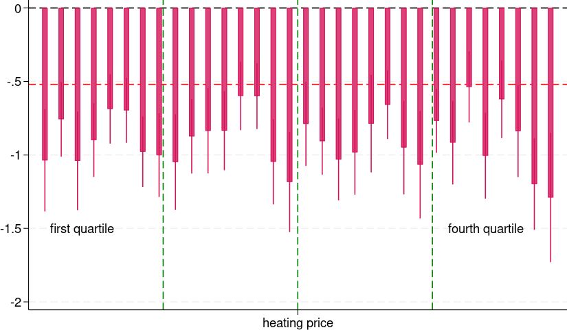
Price elasticities of heating demand at stratum level.
Higher-income households demonstrate greater heating elasticity as they usually have alternative heating systems (e.g., heating pumps) and/or better insulation.23 As a result, they have the means to react more to an increase in heating prices. This includes switching fuels or reducing (already high) thermal comfort. Additionally, poor singles and single parents are very responsive to increases in heating prices.
3.2.2. Discussion on price elasticities
As highlighted in Section 2, there is significant heterogeneity across estimates of price elasticities, depending on the energy vector, type of clients (residential vs. industrial) or time frame (short vs. long run) at stake. Moreover, as already mentioned before, most of the existing literature is based on analyses referred to the US, which, for several reasons, are not very comparable to Italy - where, on the contrary, evidence is scant - from a point of view of retail energy markets. This implies that it is very difficult to gauge whether our elasticity estimates are “too high” or “too low”.
Peersman and Wauters (2023), working on Belgium data, find that the energy price elasticity is significantly higher for price increases rather than price decreases, while it diminishes heavily for greater price hikes like the ones recently experienced by Italian households.
Additionally, the energy price variations recorded in the period, and especially in 2020-22, are so large that they might have induced a structural break, i.e. households’ responses might have become more elastic. Unfortunately, the microdata for 2023 are not yet available but only aggregate demand which reports a reduction of households’ electricity and natural gas demand by, respectively, 3.7 and 13.5 per cent with respect to 2021.
To cope with the lack of information on energy prices at the household level, we used the available sources discussed in Section 3.1 and reported in Table 1. However, as previously pointed out, millions of households in Italy were provided electricity and natural gas at fixed prices when the price surge started (end of Q2-2021). While many of these contracts have expired over time and the supply of new fixed contracts almost disappeared over 2022, it is also true that for months, some households paid less for their electricity and natural gas in 2022 than in 2020 because of the government’s interventions.
All these assumptions do not come for free. Given the price variations and our estimates of (subgroups) price elasticities, we estimate that between 2021 and 2022 overall electricity demand would have fallen between 8 (using Eurostat prices) and 14.7 (NIC) percent (w.r. to an effective 3.7 percent decrease) while the estimated heating demand between 34.8 (Eurostat) and 53.2 (NIC) percent (w.r. to an actual cut of 13.5 percent).
While a fall in demand, following a price increase is prima facie evidence of a behavioural response (and, therefore, works assuming fixed demand should be reconsidered), the differences cited above in decreased demand are striking. Only when the fully-fledged official microdata are available this puzzle will possibly be solved. Nevertheless, as the goal of this paper is to run a stress test exercise, our estimates are very good for capturing the worst-case scenario.
4. Setup of the financial vulnerability simulation
In this section, we build the modelling structure of our exercise. A household is defined as financially vulnerable if loan instalments to income exceeds 30 per cent and its income is below the median of the population.
Comparing vulnerable households with the other indebted ones indicates that the former have slimmer net wealth, much thinner financial assets, much lower income in the face of substantially higher mortgage amount. This translates in higher annual instalment as well as debt-to-income ratio for vulnerable households (Table 5). In contrast, no significant differences emerge in term of either household size or median age of the main income earner. Consumption expenditure, which includes food consumption inside and outside the home, bills, all other consumption, and travel expenses, is lower for vulnerable households with respect to the other ones.
Indicators of indebted households in 2020 (median value)
| Vulnerable HHs | Other indebted HHs | |
|---|---|---|
| Age | 49 | 49 |
| Household Size (number of components) | 3 | 3 |
| Net Wealth (euros) | 100,900 | 131,000 |
| Financial Assets (euros) | 3,000 | 10,000 |
| Debt to income | 3.6 | 0.7 |
| Debt to assets | 0.3 | 0.2 |
| Income (euros) | 15,147 | 34,474 |
| Mortgage (euros) | 52,000 | 16,000 |
| Annual debt instalment (euros) | 7,680 | 4,800 |
| Monthly consumption expenses | 1,158 | 1,416 |
-
Notes: Our calculations are based on SHIW data.
Financially vulnerable households are more likely to be late in their loan repayments by more than 90 days, which is the first stage of non-performing loans (Michelangeli and Rampazzi, 2016). This indicator is also highly correlated with the rate of new non-performing household loans based on Italy’s Central Credit Register data.24, 25 For these reasons, vulnerable households should be closely monitored to gain some insight into the threats potentially posed to the stability of the financial sector.
As for households, vulnerability from a financial stability standpoint does not necessarily mean default but refers to possible difficulties in meeting financial obligations when a negative shock occurs. Many vulnerable households are solvable if economic conditions do not change, but they could move from a state of vulnerability to one of default if their ability to repay their debts is hindered by a negative shock. We thus aim to identify indebted agents who could be problematic for their selves (for instance, they could lose their homes) as well as for the liquidity and solvability of financial intermediaries.
To analyse the problem at stake in a dynamic way, we need to make projections for several variables, namely mortgage and consumer credit instalments and debt, income and consumption, the latter variable being crucial for assessing the impact of a variation in energy prices.
4.1. Financial liabilities and income projections
Mortgages represent the main liability of Italian households and, consequently, household financial vulnerability is closely tied to changes in loan instalments associated with this type of debt. To predict mortgage loan instalments, we build on the work by Michelangeli and Pietrunti (2014) that computes the loan repayments exploiting the standard amortization formula and the household-specific debt characteristics available in the SHIW.24 The scheduled total annual repayment for any mortgage type (for instance, a household can have more than one mortgage), , of household at time is given by:
where is the interest rate on debt and is the residual duration.
Starting in 2014, consumer credit in Italy began skyrocketing and it was warranted to take properly into account any consumer loans in Bank of Italy’s microsimulation model.25 To this end, we rely on the approach proposed by Attinà et al. (2020), according to which the projection of consumer credit is achieved in three steps. In the first step, household participation in the consumer credit market is estimated by exploiting the following regression:
where is a dummy variable equal to one if household has a consumer loan in year and zero otherwise, is a dummy variable equal to one if household has a mortgage loan in year and zero otherwise, is a vector of income quartile dummies, is a vector of household durable consumption dummies.
In the second step, the change in the total amount of consumer credit is forecast running the following regression:
where is the growth rate of consumer loans to households in the Italian economy.
Finally, the instalment paid by each household is computed assuming a standard amortization scheme.
Regarding income projections, we rely again on the approach presented in Michelangeli and Pietrunti (2014). Households are differentiated according to their income class. For each income class, the parameters of the income process (mean and variance) are estimated using historical microeconomic data and households’ income can be diverse reflecting different income realizations. The process for the growth of disposable income for each class is given by:
The debt and income growth generated by the model is then required to be consistent with the growth in household debt and nominal income from macroeconomic projections.
4.2. Consumption projections
Building on Faiella et al. (2022), we aim to assess how the change in energy prices, induced by a combination of supply and demand factors in 2021 and the Russian invasion of Ukraine in 2022, affected households’ financial vulnerability, via higher energy expenses. To this end, we expand the Bank of Italy microsimulation models of household financial vulnerability to project household consumption evolution. We start from each i-th household consumption in period t-1, ; we multiply this by the annual growth recorded for the stratum to which household i belongs, :26
We then aggregate consumption over the entire population and scale it by an adjustment factor, , to make sure that changes in aggregate consumption stemming from the model match those coming from macroeconomic projections resulting from the proprietary model of the Bank of Italy.
At this stage, each household in our model has its debt, income and consumption over the simulation period.
4.3. Households vulnerability in presence of energy price shocks
In this subsection, we put together all the pieces so far elaborated. We take the changes in expenditure induced by the higher energy prices for each stratum, and join this information with the Bank of Italy’s 2020 SHIW microdata, using stratum as the merging key.
We then assume that households’ available income is modified as a consequence of the change in total expenditure triggered by the shock in energy prices. The new household income will be different across households as it will depend on their energy elasticities and consumption levels and how those could change in response to the shock. To account for energy price changes in the scenario (see Table 1), let income (gross of financial charges and net of imputed rents) of household belonging to stratum be modified as follows:
where is household consumption, and is an adjustment factor equal to the ratio of total consumption after and before the change in energy price. In case there is no energy price shock, goes to 1 and equals .
Against these assumptions, the indicator for household financial vulnerability, , which now accounts for the effects on income of higher energy prices, is defined as follows:
where is household total loan instalment (given by the sum of mortgage and consumer credit instalments) in year , and () is the median value of equalized income in the population in period , adjusted to take into account the effect of the energy price change.
4.4. Data used in the model of households’ financial vulnerability
In this section, we present the data used in the microsimulation model of household vulnerability. We acknowledge that the baseline scenario, which does not account for energy price shock, spans until 2023; the other scenarios, which instead incorporate also energy shocks, are available only up to 2022.
The household-level data used as a starting point of the microsimulation model are from the most recent SHIW wave, namely 2020.27
The microsimulation model then simulates dynamics for total income, total debt, consumption and interest rates that are in line with the macroeconomic environment or with its forecasts according to the Bank of Italy projections of April.28
Macro data come from several sources. First, we use disposable income (growth) from the national accounts (Contabilità Nazionale, CN), which includes imputed rents and is aimed at capturing the standard of living of households.29 After plummeting in 2020 as a consequence of the repercussions of the Covid-19 pandemic, income rebounded in 2021 (its growth was 3.5 per cent) and accelerated further in 2022 (at 6.3 per cent); income expansion is projected to soften in 2023, but to remain moderately positive. Second, we make use of the historical evolution and projections of lending to households for house purchases and for consumer credit - which are from the Bank of Italy’s statistical data warehouse. Mortgages growth was high in 2021 and 2022 (at around 5 per cent in both years) but it was expected to slow down sharply in 2023; a similar trend, although somewhat more subdued, is shown for consumer credit (granted by banks).30 We use actual data and projections of the three-month Euribor obtained from futures contracts to recalculate payments of households holding a variable interest rate mortgage and those associated with new originations. At the same time, we exploit the 10-year IRS as a benchmark for fixed-rate new mortgages. While in 2021 the Euribor further declined to -0.547 per cent (annual average), it was slightly positive in 2022 (0.343 per cent) and was expected to increase sharply in 2023. On average in 2021 the IRS stood at little more than zero per cent, but increased sharply in 2022 (to 1.9 per cent); for 2023 the IRS growth could be slightly lower. We finally exploit both HBS data to compute the change in consumption expenditure by stratum and the macroeconomic projections on yearly growth of final consumption from the internal Bank of Italy macroeconomic model to generate aggregate consumption dynamics in the model similar to those observed in the data. The yearly variations in final consumption are around 5 per cent in the year 2021-22 and are projected to be lower in 2023.
5. Results
This section presents the model results. We start by showing the baseline scenario, where there are no energy price shocks. We then take on board such shocks by applying the energy price changes. We repeat this exercise in two cases. In the first one, households do not adjust their consumption bundle to price increases and keep consuming the same quantities of energy goods despite the price shock, i.e. we assume no price elasticity; in the second case, households change their consumption habits to fight back against price hikes, i.e. we use previously estimated price elasticities per stratum. Given the lack of more granular information on prices, we assume that in each scenario all households face the same energy price increases, which is likely not the case in reality. This renders the results of the exercise an upper bound for households’ vulnerability since, in the spirit of a stress test, as we have seen above in Section 3, the majority of consumers have multi-year contracts.
5.1. Baseline
For the baseline scenario, the debt at risk decreases in 2021-22 and records a slight increase in 2023 (Figure 3). Such dynamics reflect the evolution of the macroeconomic drivers as described in Section 3.2: in 2021-22 the sustained recovery in nominal disposable income overcame the evolution of households’ liabilities, driving households’ vulnerability on a downward path.31 In 2023 the increased debt at risk would therefore be mainly attributable to the abrupt rise in loan rates following the change in monetary policy stance implemented to fight the inflation spike.

Baseline.. Notes: The figure shows the share of vulnerable households and the debt at risk in the baseline model. The rate of new non-performing household loans is defined as the ratio of non-performing loans to total household loans at the beginning of the period and it is calculated as an average of the quarters; the ratio is available until 2022.
5.2. Case 1 (no elasticity): households not re-adjusting their consumption after the shock
We consider a model where households’ income and debt evolve over time reflecting macroeconomic developments, but with households not readjusting their quantity of energy consumed following the yearly price increases. Therefore, households’ energy expenditure increases after the shock by an amount equal to the price change multiplied by the consumption level. Panel (a) in Figure 4 and Panels (A) and (B) in Table 6 show expenditure and income variations. The dots in Figure 4 represent the average ratio between the total household consumption expenses after and before the energy shock, , while the bars show the average disposable income adjusted to take into account the eventual re-composition of household expenses occurring as a consequence of the energy price shock. Averages are computed across different simulations.
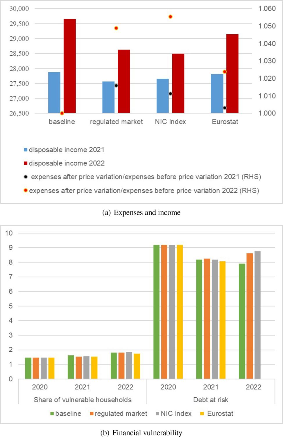
Microsimulation model with no price elasticity (case 1): Aggregate results.. Notes: Panel (a) shows how household consumption and disposable income change, on average, after the energy price shock. Panel (b) reports the share of vulnerable households and their debt (debt at risk). Disposable income is in euros, and results for Panel (b) are in percentage values.
Model with no price elasticity (case 1): Aggregate results.
| 2020 | 2021 | 2022 | |
|---|---|---|---|
| (1) | (2) | (3) | |
| A. Expenses after /Expenses before | |||
| baseline | 1.000 | 1.000 | |
| regulated market | 1.016 | 1.049 | |
| NIC Index | 1.011 | 1.055 | |
| Eurostat | 1.003 | 1.024 | |
| B. Disposable income | |||
| baseline | 26,882 | 27,884 | 29,652 |
| regulated market | 26,882 | 27,564 | 28,630 |
| NIC Index | 26,882 | 27,656 | 28,493 |
| Eurostat | 26,882 | 27,820 | 29,149 |
| C. Share of vulnerable households | |||
| baseline | 1.45 | 1.62 | 1.80 |
| regulated market | 1.45 | 1.54 | 1.82 |
| NIC Index | 1.45 | 1.55 | 1.85 |
| Eurostat | 1.45 | 1.53 | 1.74 |
| D. Debt at risk | |||
| baseline | 9.19 | 8.18 | 7.90 |
| regulated market | 9.19 | 8.25 | 8.62 |
| NIC Index | 9.19 | 8.18 | 8.75 |
| Eurostat | 9.19 | 8.07 | 8.15 |
-
Notes: Panel A shows households’ consumption average change after the energy price shock; Panel B reports disposable income in euros; Panels C and D include the share of vulnerable households and their debt at risk in percentage values.
In the baseline scenario, by construction, nothing changes. In 2021 and 2022 expenses are the same before and after the shock and the ratio equals 1. In 2021, across the different scenarios that account for the energy price shocks, reductions in disposable income concerning baseline are contained (between 60 and 320 euros). This reflects the limited increase in energy prices and the consequent limited additional expenses to maintain constant the quantity consumed. On the opposite, the increase in energy expenses is rather pronounced in 2022, ranging from 2.4 to 5.5 per cent across scenarios. Households’ disposable income dropped markedly, up to 1,150 euros.
Panel (b) in Figure 4 and Panels (C) and (D) in Table 6 show the impact of energy price changes on households’ financial vulnerability in the baseline scenario and under the three alternative scenarios. The decrease in disposable income, by limiting the available financial resources that can be used to service the debt, hurts financial vulnerability. In 2021, in the three scenarios, financial vulnerability is about the same as the one recorded in the baseline scenarios, reflecting the contained growth in energy expenses. In 2022, instead, debt at risk increases with respect to 2021 across the three scenarios considered. The increase turns out to be stronger when the energy price upsurge is measured by the NIC Index - which recorded the highest increase - but, under any scenarios, we observe the same dynamics. This non-monotonic evolution of the debt at risk is inconsistent with the one for the new rate of non-performing loans, which continued to decrease in 2021 and 2022, highlighting that some important readjustment has taken place in actual data.
5.3. Case 2 (with price elasticity): households re-adjusting their consumption after the shock
We now consider a far more realistic, yet less studied, case where, in the face of an energy price shock, households re-adjust their yearly consumption depending on their price elasticity.
5.3.1. Aggregate results
As shown in Table 1, energy price variations are overall contained between 2020 and 2021 and are practically unchanged when they are computed using the Eurostat price measure. As a consequence, when the latter is employed, almost all households choose to accommodate the price raise with slightly higher expenses, bearing a negligible impact on disposable income (decreasing on average by less than 20 euros; Panel (a) of Figure 5 and Table 7). In the cases of the NIC Index or regulated market, larger price variations are associated with more marked expenses and a deeper, but still moderate, decline in average income (around 100 euros) with respect to the baseline.
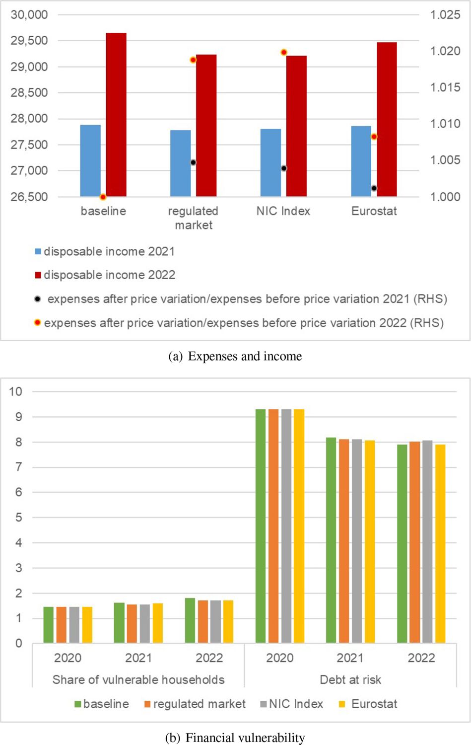
Microsimulation model with price elasticity, (case 2): Aggregate results.. Notes: Panel (a) shows how household consumption and disposable income change, on average, after the energyprice shock. Panel (b) reports the share of vulnerable households and their debt (debt at risk). Disposable incomeis in euros, and results for Panel (b) are in percentage values.
Model with price elasticity (case 2): Aggregate results.
| 2020 | 2021 | 2022 | |
|---|---|---|---|
| (1) | (2) | (3) | |
| A. Expenses after /Expenses before | |||
| baseline | 1.000 | 1.000 | |
| regulated market | 1.005 | 1.019 | |
| NIC Index | 1.004 | 1.020 | |
| Eurostat | 1.001 | 1.008 | |
| B. Disposable income | |||
| baseline | 26,882 | 27,884 | 29,652 |
| regulated market | 26,882 | 27,785 | 29,238 |
| NIC Index | 26,882 | 27,801 | 29,207 |
| Eurostat | 26,882 | 27,860 | 29,470 |
| C. Share of vulnerable households | |||
| baseline | 1.45 | 1.62 | 1.80 |
| regulated market | 1.45 | 1.54 | 1.71 |
| NIC Index | 1.45 | 1.54 | 1.72 |
| Eurostat | 1.45 | 1.59 | 1.72 |
| D. Debt at risk | |||
| baseline | 9.30 | 8.18 | 7.90 |
| regulated market | 9.30 | 8.10 | 8.02 |
| NIC Index | 9.30 | 8.10 | 8.06 |
| Eurostat | 9.30 | 8.06 | 7.91 |
-
Notes: Panel A shows households’ consumption average change after the energy price shock; Panel B reports disposable income in euros; Panels C and D include the share of vulnerable households and their debt at risk in percentage values.
Energy price variations are instead more pronounced over the period 2021-2022. Under any scenarios considered, households increase their average consumption expenditure in the range of 0.8-2.0 per cent.32 Notwithstanding differences in the extent of price hikes across scenarios, price spikes seem to have a linear impact on total expenditure. Hence, it appears that the price-triggered expenditure increase in the NIC and regulated market scenarios - which are more than twice as big as Eurostat’s (see Table 1) - drives a more pronounced consumption correction. The ensuing decrease in disposable income is in the range of 180 to 450 euros.
Household vulnerability does not go up following the rise in energy prices. Throughout any scenarios, the share of vulnerable households and the debt at risk appear to be about the same as that prevailing in the baseline (Panel (b) of Figure 5), suggesting that indebted households, in particular, adjust their consumption patterns in such a way as to keep a level of disposable income as unchanged as possible to be used also for debt repayments. Again, while the energy price increase does not lead to higher financial vulnerability, household welfare could have suffered a blow as a consequence of the cut in energy consumption.
The result on financial vulnerability measured by the debt at risk is very much in line with the evidence from the rate of new non-performing loan ratio based on supervisory reports (Figure 3). The debt at risk is confirmed to be an indicator with similar dynamics to the new non-performing loan ratio and, thus, it can be used to forecast the evolution of vulnerability.
5.3.2. Heterogeneity results
Tables 8 and 9show the results for the models by considering the heterogeneity across the three dimensions, namely geographical areas, number of household components and age classes. Against a backdrop of energy price shocks having a more marked impact in 2022, the higher the inflation shock, the more likely households to re-adjust their consumption habit. As a consequence of the consumption correction, disposable income is hit less. In general, taking on board consumption re-adjustment - which reflects the coming into play of the energy price elasticities - brings about limited effects in financial vulnerability. Concerning any of the heterogeneity dimensions considered, the energy price changes overall have a homogeneous impact.33
Model with price elasticity (case 2): heterogeneity in expenses and disposable income.
| Expenses after/Expenses before | Disposable income | |||||
|---|---|---|---|---|---|---|
| (1) | (2) | (3) | (4) | (5) | (6) | |
| Geographical area | ||||||
| North | Center | South | North | Center | South | |
| 2020 | ||||||
| baseline | 31,161 | 28,138 | 20,094 | |||
| 2021 | ||||||
| baseline | 1.000 | 1.000 | 1.000 | 32,341 | 29,201 | 20,813 |
| regulated market | 1.003 | 1.004 | 1.006 | 32,239 | 29,107 | 20,717 |
| NIC Index | 1.004 | 1.004 | 1.005 | 32,255 | 29,123 | 20,734 |
| Eurostat | 1.001 | 1.001 | 1.001 | 32,316 | 29,178 | 20,790 |
| 2022 | ||||||
| baseline | 1.000 | 1.000 | 1.000 | 34,414 | 31,063 | 22,097 |
| regulated market | 1.017 | 1.017 | 1.022 | 33,991 | 30,661 | 21,688 |
| NIC Index | 1.017 | 1.018 | 1.024 | 33,966 | 30,633 | 21,646 |
| Eurostat | 1.007 | 1.008 | 1.010 | 34,226 | 30,889 | 21,917 |
| Number of household components | ||||||
| 1-2 | 3 | 4+ | 1-2 | 3 | 4+ | |
| 2020 | ||||||
| baseline | 21,280 | 33,598 | 37,186 | |||
| 2021 | ||||||
| baseline | 1.000 | 1.000 | 1.000 | 22,080 | 34,858 | 38,543 |
| regulated market | 1.005 | 1.005 | 1.005 | 22,000 | 34,738 | 38,412 |
| NIC Index | 1.004 | 1.004 | 1.004 | 22,016 | 34,754 | 38,429 |
| Eurostat | 1.001 | 1.001 | 1.001 | 22,062 | 34,828 | 38,510 |
| 2022 | ||||||
| baseline | 1.000 | 1.000 | 1.000 | 23,488 | 37,066 | 40,969 |
| regulated market | 1.018 | 1.020 | 1.019 | 23,146 | 36,560 | 40,429 |
| NIC Index | 1.018 | 1.023 | 1.022 | 23,140 | 36,492 | 40,355 |
| Eurostat | 1.008 | 1.010 | 1.009 | 23,348 | 36,831 | 40,711 |
| Age classes | ||||||
| 15-39 | 40-65 | 66+ | 15-39 | 40-65 | 66+ | |
| 2020 | ||||||
| baseline | 27,611 | 30,218 | 21,803 | |||
| 2021 | ||||||
| baseline | 1.000 | 1.000 | 1.000 | 27,970 | 31,569 | 22,959 |
| regulated market | 1.005 | 1.005 | 1.005 | 27,870 | 31,461 | 22,874 |
| NIC Index | 1.004 | 1.004 | 1.004 | 27,885 | 31,477 | 22,891 |
| Eurostat | 1.001 | 1.001 | 1.001 | 27,945 | 31,542 | 22,939 |
| 2022 | ||||||
| baseline | 1.000 | 1.000 | 1.000 | 29,111 | 33,572 | 24,749 |
| regulated market | 1.018 | 1.018 | 1.019 | 28,703 | 33,120 | 24,382 |
| NIC Index | 1.020 | 1.020 | 1.020 | 28,666 | 33,068 | 24,378 |
| Eurostat | 1.008 | 1.008 | 1.008 | 28,925 | 33,364 | 24,599 |
-
Notes: Columns 1-3 show household consumption average change after the energy price shock. Columns 4-6 report disposable income in euros.
Model with price elasticity (case 2): heterogeneity in financial vulnerability.
| Share of vulnerable households | Debt at risk | |||||
|---|---|---|---|---|---|---|
| (1) | (2) | (3) | (4) | (5) | (6) | |
| Geographical area | ||||||
| North | Center | South | North | Center | South | |
| 2020 | ||||||
| baseline | 1.41 | 1.45 | 1.52 | 8.86 | 6.51 | 16.51 |
| 2021 | ||||||
| baseline | 1.50 | 1.08 | 2.12 | 7.36 | 4.85 | 16.30 |
| regulated market | 1.30 | 1.11 | 2.14 | 7.36 | 4.41 | 16.43 |
| NIC Index | 1.30 | 1.11 | 2.14 | 7.36 | 4.31 | 16.42 |
| Eurostat | 1.43 | 1.08 | 2.12 | 7.34 | 4.36 | 16.32 |
| 2022 | ||||||
| baseline | 1.50 | 1.38 | 2.49 | 6.52 | 5.25 | 16.03 |
| regulated market | 1.31 | 1.39 | 2.48 | 6.58 | 5.18 | 16.60 |
| NIC Index | 1.31 | 1.39 | 2.48 | 6.62 | 5.20 | 16.66 |
| Eurostat | 1.29 | 1.39 | 2.53 | 6.51 | 5.09 | 16.32 |
| Number of household components | ||||||
| 1-2 | 3 | 4+ | 1-2 | 3 | 4+ | |
| 2020 | ||||||
| baseline | 0.80 | 2.13 | 2.77 | 8.69 | 9.87 | 9.45 |
| 2021 | ||||||
| baseline | 1.28 | 1.62 | 2.63 | 9.35 | 7.57 | 7.36 |
| regulated market | 1.11 | 1.64 | 2.73 | 8.99 | 7.61 | 7.48 |
| NIC Index | 1.11 | 1.64 | 2.73 | 8.99 | 7.61 | 7.48 |
| Eurostat | 1.21 | 1.63 | 2.67 | 9.01 | 7.58 | 7.38 |
| 2022 | ||||||
| baseline | 1.40 | 2.16 | 2.68 | 9.68 | 7.37 | 6.47 |
| regulated market | 1.20 | 2.19 | 2.80 | 9.57 | 7.52 | 6.77 |
| NIC Index | 1.19 | 2.19 | 2.83 | 9.56 | 7.58 | 6.84 |
| Eurostat | 1.24 | 2.17 | 2.73 | 9.50 | 7.45 | 6.60 |
| Age classes | ||||||
| 15-39 | 40-65 | 66+ | 15-39 | 40-65 | 66+ | |
| 2020 | ||||||
| baseline | 2.66 | 1.95 | 0.26 | 12.36 | 7.70 | 13.38 |
| 2021 | ||||||
| baseline | 2.17 | 2.29 | 0.56 | 10.81 | 7.34 | 6.36 |
| regulated market | 2.17 | 2.32 | 0.30 | 10.82 | 7.28 | 5.63 |
| NIC Index | 2.17 | 2.32 | 0.30 | 10.82 | 7.28 | 5.63 |
| Eurostat | 2.17 | 2.29 | 0.46 | 10.81 | 7.19 | 6.11 |
| 2022 | ||||||
| baseline | 2.20 | 2.56 | 0.73 | 11.27 | 7.05 | 5.62 |
| regulated market | 2.51 | 2.50 | 0.49 | 12.42 | 6.96 | 5.02 |
| NIC Index | 2.51 | 2.51 | 0.49 | 12.46 | 7.00 | 5.02 |
| Eurostat | 2.30 | 2.57 | 0.48 | 11.64 | 7.01 | 5.01 |
-
Notes: The share of vulnerable households and the debt at risk are in percentage values.
6. Conclusions
During 2021 retail prices of electricity and natural gas increased significantly owing to a mismatch of supply and demand; such dynamics were exacerbated by the Russian invasion of Ukraine in February 2022. The price surge could possibly jeopardize households’ welfare and financial soundness, especially in countries like Italy, where prices more than doubled in a short time.
Against this backdrop, we have developed a microsimulation model to evaluate the impact of the upsurge in energy prices on households’ financial vulnerability. This paper builds on previous works of Michelangeli and Pietrunti (2014); Attinà et al. (2020); Faiella and Lavecchia (2021b) and Faiella et al. (2022). For the period 2020-2022, we show that by turning a blind eye to consumers’ behavioural responses (i.e. assuming price inelasticity, a common assumption in the literature), households’ financial vulnerability may be significantly overestimated and its dynamics are not aligned with banks’ supervisory report data on the new rate of non-performing household loans. Conversely, by taking energy demand price elasticities into due account along with the evolution of the relevant macro variables, we find that the increase in the number of vulnerable households (and their associated indebtedness) is comparable to the rise recorded in a scenario where energy prices do not change and more in line to what has broadly occurred in reality. This is because households readjust their energy consumption levels (i.e., they trim their use of electricity and heating) to maintain a constant level of disposable income so that it can be used to service their debt.
Some caveats to the exercise results apply, though. First, and foremost, we performed a partial equilibrium analysis focused on energy markets only and the impact of energy price increases on household financial vulnerability; as a consequence, this exercise has to be interpreted as a stress test. Second, we are aware that there are differences in elasticity values in the presence of price rises or falls and that the 2021-22 episode marked an inflation spike not recorded in many years; at the same time, the nearness of the price surge to the current date prevents the availability of newer data; in addition, its short duration suggests that it would be safe to assume an unchanged energy price elasticity before and after the price spike. At the same time, in light of the magnitude of the price shock, structural breaks in elasticity can not be ruled out. Be as it may, in case of higher elasticity, we would converge towards a case with limited effect on households’ financial vulnerability, but heftier repercussions on welfare. Results would be still driven by the evolution of macro variables. Finally, we are focusing on energy expenditure, but other consumption items, such as food items, incurred large price increases. However, assessing a rebalancing in households’ consumption basket would require information on cross-price and income elasticities for any goods. This information is not available at the current stage and we leave it for future research.
We can then conclude that, if the energy price change did not lead to higher financial vulnerability, this is not a free lunch. Households forgo thermal comfort, potentially experiencing an increase in energy poverty (Faiella and Lavecchia, 2021a; OIPE, 2023), to keep within their budget constraints.
Footnotes
1.
IEA, “What is behind soaring energy prices and what happens next?”, commentary, 12 October 2021.
2.
At the end of 2021, Italy’s natural gas imports from Russia accounted for about 40 per cent of the total, standing at just slightly less than 29 billion cubic meters.
3.
The surge in final energy prices, driven by spikes in import prices of natural gas, affected also the trade balance, with an energy trade deficit peaking at 5.4 per cent of GDP in 2022, the second-highest on record since 1981; the trade balance deterioration (3 percentage points of GDP) was slightly larger than those observed after the oil shocks of the 1970s (Romanini and Tosti, 2023).
4.
At the end of 2023, the energy component accounted for 60 per cent of the final price of electricity paid by households, the other 40 per cent was made up of taxes, levies and distribution fees (for gas, the energy component accounts for an even smaller share, circa 50 per cent). Taxes, levies and distribution fees are set by ARERA, while only the energy component is determined by the market.
5.
Since October 2022, gas prices are updated monthly.
6.
The historical evolution of income includes all the government measures implemented in 2021-22 to mitigate inflation effects on household budgets.
7.
Excluding behavioural responses is a rather common, albeit counter-intuitive, assumption across microsimulation models (UPB, 2022; Istat, 2022; Curci et al. 2022). Moreover, as a consequence of the price surge in 2022 households' demand for electricity decreased by 3.6 (4.6) per cent with respect to 2021 (2020), while that for natural gas fell by 9.5 (1.7) per cent compared to 2021 (2020).
8.
In the paper we focus on financially vulnerable families. In 2020-22, Italian households accumulated a substantial amount of additional financial assets – in the order of more than 130 euro billion – as a consequence of the repercussions of the COVID-19 pandemic on the economy. At the same time, the distribution of financial wealth in Italy like in other countries is skewed towards the better-off, as so it was the distribution of additional savings. Additionally, the debt-to-income ratio in the same period remained almost unchanged. Hence, it appears that savings drawing down played, if any, a marginal role (Colabella et al., 2023).
9.
10.
11.
Natural gas covers, on average, 60 per cent of the space heating uses. Moreover, data on retail prices for the other energy vectors used for space heating (wood, pellet, district heating, LNG, gas cylinders, etc.) are unavailable, not even at the aggregate level. Therefore, in the absence of better data, we will assume that the retail prices of natural gas work as a proxy for all the heating fuels (the remaining 40 per cent).
12.
Directive 96/92/EC (``first electricity Directive"), adopted in 1996, and Directive 98/30/EC (``first gas directive"), adopted in 1998.
13.
Data for the electricity can be recovered from ARERA website. Also, we employed the following conversion factor from standard cubic meter (smc in Italian) to GJ: 1 smc = 0.0394 Gj.
14.
The price indexes for the regulated market reflect the quarterly updates by ARERA to its tariffs, whilst the price indexes for the free market refer to new contracts only and, hence, apply to a fraction of customers, who have signed a new deal with an energy provider. More than 70 per cent of households on the free market (i.e. almost 50 per cent of all households) have multi-year, fixed-price contracts; therefore, such households are unaffected as long as their contracts do not expire. At the current juncture, information on contract length for households is unavailable.
15.
Data can be recovered from here.
16.
As the NIC serves as a price index, we calculate the absolute variations by applying the cumulative percentage changes to the corresponding base year from Eurostat. For example, to estimate the average electricity price in 2020, we apply the electricity price variation from the NIC between 2019 and 2020 to the 2019 average price from Eurostat.
17.
See UPB (2023), chapter 5.3, for greater detail.
18.
Indagine sui consumi delle famiglie for the years between 1997 and 2013 and the Indagine sulla spesa delle famiglie from 2014 to 2022. In this paper we use data from 1997 to 2022.
19.
As mentioned above, we use natural gas price as the reference price for overall heating expenditure.
20.
Our model estimates energy quantities at the household level, calibrating the yearly final estimate with overall electricity and heating consumption. This calibration is based on national energy balances from 1997 to 2008, Eurostat’s Physical Energy Flow Accounts (PEFA) from 2008 to 2021, and official variations from ARERA for 2022.
21.
The quasi-panel approach compares the values of population subgroups classified in different stratum formed according to their demographic characteristics (i.e. age, marital status, number of family components). The authors use the household classification provided by Istat, accruing to eight subgroups of households, observed across fourths of the equivalent expenditure distribution (e.g. households belonging to the fourth quartile of the equivalent expenditure distribution, are recorded as 4xx.).
22.
Namely, we merge households with 3 or more children within households with 2 children because of the relatively scarce number of observations.
23.
We assume total equivalent expenditure as a proxy for wealth.
24.
In addition to imposing some structure for the evolution of debt for existing mortgages, Michelangeli and Pietrunti (2014) present a way of introducing mortgage originations, which result from a pseudo-panel that builds on historical data and are adjusted to match the total growth in household debt available from macroeconomic forecasts. The number of new loans attributed to each income class is thus endogenously determined in line with the macroeconomic assumptions. The model assumes that 50 per cent of the originations have a variable mortgage rate while the rest have a fixed mortgage rate.
25.
Attinà et al. (2020) show that about half of vulnerable households have some kind of consumer credit and these loans represent a larger threat to financial stability when associated with mortgages.
26.
For 2021-22, we use the average growth of total consumption per stratum from the HBS. For 2023, we use the average growth per stratum between 2016 and 2019.
27.
This survey has been carried out since the 1960s. The dataset contains detailed information on households’ characteristics (e.g. number of household members, age, residence), income, debt (distinguishing between mortgage and consumer credit) and consumption. For a description of the survey, see Survey on Household Income and Wealth.
28.
For details on the projections of Bank of Italy see Bollettino economico 1/2023.
29.
By definition disposable income in 2021 and 2022 includes all the fiscal measures in favour of households aimed at staving off inflation effects on their financial balances, such as targeted transfers.
30.
Consumer credit growth was 1.0 and 2.9 per cent, respectively in 2021 and 2022, while a moderate slowdown is expected in 2023.
31.
Starting from 2021, households' income has also been propped up by government’s measures aimed at helping most-in-need households ease pressure on their balances stemming from the energy price surge. See 3 for greater detail.
32.
This bracket is smaller than the one prevailing in the case of no elasticity indicating that households decide to accommodate price increases up to a certain extent.
33.
There is no material difference in the evolution of disposable income, consumption and vulnerability between households that in 2020 were vulnerable and those who were not. Details are available on request.
References
-
1
Modelling households’ financial vulnerability with consumer credit and mortgage renegotiationsInternational Journal of Microsimulation 13:67–91.https://doi.org/10.34196/ijm.00213
-
2
Number 1 in Financial stability report. Bank of EnglandNumber 1 in Financial stability report. Bank of England.
- 3
-
4
Working papers, Universita degli Studi di FirenzeWorking papers, Universita degli Studi di Firenze.
-
5
Electricity Demand Elasticity in ItalyAtlantic Economic Journal 40:439–440.https://doi.org/10.1007/s11293-012-9331-5
- 6
- 7
- 8
-
9
Questioni di Economia e Finanza (Occasional Papers) 738, Banca d’ItaliaQuestioni di Economia e Finanza (Occasional Papers) 738, Banca d’Italia.
-
10
Panel data from time series of cross-sectionsJournal of Econometrics 30:109–126.https://doi.org/10.1016/0304-4076(85)90134-4
-
11
Comparative analysis of different techniques to impute expenditures into an income data setInternational Journal of Microsimulation 13:70–94.https://doi.org/10.34196/IJM.00226
-
12
Turning on the Lights: A Meta-Analysis of Residential Electricity Demand ElasticitiesJournal of Agricultural and Applied Economics 36:1–17.https://doi.org/10.1017/S1074070800021866
- 13
-
14
Energy poverty. How can you fight it, if you can’t measure it?Energy and Buildings 233:110692.https://doi.org/10.1016/j.enbuild.2020.110692
-
15
Questioni di Economia e Finanza (Occasional Papers) 614, Bank of ItalyQuestioni di Economia e Finanza (Occasional Papers) 614, Bank of Italy.
- 16
-
17
A climate stress test on the financial vulnerability of Italian households and firmsJournal of Policy Modeling 44:396–417.https://doi.org/10.1016/j.jpolmod.2021.11.001
-
18
Analysis of individual natural gas consumption and price elasticity: Evidence from billing data in ItalyEnergy Economics 118:106484.https://doi.org/10.1016/j.eneco.2022.106484
- 19
-
20
Burden of the global energy price crisis on householdsNature Energy 8:304–316.https://doi.org/10.1038/s41560-023-01209-8
-
21
Some Calculations on Electricity Consumption in Great BritainJournal of the Royal Statistical Society. Series A (General) 114:359–371.https://doi.org/10.2307/2980781
- 22
-
23
A meta-analysis on the price elasticity of energy demandEnergy Policy 102:549–568.https://doi.org/10.1016/j.enpol.2017.01.002
-
24
A Microsimulation Model to evaluate Italian Households’ Financial VulnerabilityInternational Journal of Microsimulation 7:53–79.https://doi.org/10.34196/ijm.00107
-
25
Questioni di Economia e Finanza (Occasional Papers) 369, Banca d’ItaliaQuestioni di Economia e Finanza (Occasional Papers) 369, Banca d’Italia.
- 26
-
27
Annual report, Osservatorio italianosulla poverta energeticaAnnual report, Osservatorio italianosulla poverta energetica.
- 28
- 29
-
30
Managing the liberalization of Italy’s retail electricity market: A policy proposal☆Energy Policy 137:1–6.https://doi.org/10.1016/j.enpol.2019.111150
-
31
Technical report, Ufficio parlamentare di bilancioTechnical report, Ufficio parlamentare di bilancio.
-
32
Technical report, Ufficio parlamentare di bilancioTechnical report, Ufficio parlamentare di bilancio.
Article and author information
Author details
Acknowledgements
We would like to thank, Alessio Anzuini, Andrea Bonfatti, Stefano Clò, Nicola Curci, Alessio De Vincenzo, Ivan Faiella, Giovanni Guazzarotti, Sara Meservey, Patrizio Pagano, Sabrina Pastorelli, Corrado Pollastri, Luigi Federico Signorini and three anonymous referees. Also, participants to the Bank of Italy's 2nd Workshop on Microsimulation Modelling (16 June 2023), Energy and Climate Change workshop (15 December 2023), the Network for Greening the Financial System (NGFS) EN Research lunch webinar (27 September 2023), the 7th Green Finance Research Advances (GFRA - 12 December 2023), and to the seminar of the G7 Climate Change Mitigation Working Group (CCMWG; 27 October 2023) for their insightful suggestions. The views expressed herein are those of the authors and do not necessarily reflect those of the Bank of Italy.
Publication history
- Version of Record published: February 14, 2025 (version 1)
Copyright
© 2025, Colabella et al.
This article is distributed under the terms of the Creative Commons Attribution License, which permits unrestricted use and redistribution provided that the original author and source are credited.