SimPaths: An open-source microsimulation model for life course analysis
- Centre for Microsimulation and Policy Analysis, United Kingdom
- MRC/CSO Social & Public Health Sciences Unit, United Kingdom
Abstract
The paper introduces SimPaths, an open-source framework for individual and household life course events. The framework is designed to project life histories through time, building up a detailed picture of career paths, family (inter)relations, health, and financial circumstances. The modular nature of the SimPaths framework is designed to facilitate analysis of alternative assumptions concerning the tax and benefit system, sensitivity to parameter estimates and alternative approaches for projecting labour/leisure and consumption/savings decisions. SimPaths builds upon standardised assumptions and data sources, which facilitates adaptation to alternative countries – models based on the framework currently exist for the UK, Greece, Hungary, Italy, and Poland, and are under development for Germany, Spain and Sweden. Projections for a workhorse model parameterised to the UK context are reported, which closely reflect observed data throughout a validation window between the Financial crisis (2011) and the Covid-19 pandemic (2019).
1. Introduction
The demographic transition currently unfolding across the world has profound implications for diverse aspects of societies, including the functioning and financing of the welfare state. As baby boomers (those born in the two decades after WWII) move out of work and into retirement and are replaced by smaller cohorts of working-age individuals, the shares of national populations in employment are projected to decline, which will reduce public tax receipts at the same time as needs in terms of health care and social assistance are projected to rise.
The old-age dependency ratio (the population aged 65 and over, relative to the population aged 20 to 64) of OECD countries doubled from 14% in 1950 to 30% in 2020 and is projected to double again to 59% by 2075.1 Although increases in age dependency ratios are anticipated in all OECD countries, there is substantial cross-country variation. Korea is an outlier in this series, projected to rise from the lowest dependency ratio in 1950 (6%) to the highest in 2075 (79%). EU countries also feature prominently in the transition, accounting for eight of the ten countries with the highest projected age dependency ratios in the OECD by 2075.
The current rises in age dependency ratios are driven by unprecedented declines in fertility and rises in life expectancy, as well as the ageing of the baby boom generation. The OECD average total fertility rate fell by more than half from 3.3 children per woman in 1960 to 1.6 children in 2020.2 During this same period, the total fertility rate in EU countries fell from 2.6 to 1.5, and from 6.0 to 0.8 in South Korea. Furthermore, average life expectancy at birth in OECD countries increased from 68.1 years in 1960 to 80.5 years in 2020, from 69.7 to 79.9 years in EU countries, and in Korea from 58.7 years in 1970 to 80.5 years in 2020.3
These remarkable shifts in fertility and life expectancy have a pervasive bearing on social and private organisation. From partner relations to education decisions, labour market participation to housing demand, changing gender roles, caring needs, and healthcare provisions; few aspects of modern life are left unaffected. With longer lives, inequalities in income, wealth and health also have more time to compound. In short, OECD countries are passing through a period of social revolution.4
Many current trends are now well established, displaying predictable patterns over time. The influence that these trends have on margins of concern are also often predictable. For example, an older population implies a greater prevalence of old-age pensions in payment and more demand for health care, both of which impose a burden on the public purse. Yet, to move beyond basic postulations, numerical analyses are required. This is particularly true when attempting to take into consideration multiple inter-related temporal trends.
Most numerical approaches used to anticipate the scale and scope of population ageing provide limited detail for exploring distributional effects at a given point in time, longitudinal effects over individual life courses, and implications for financing of the welfare state. The European Commission and OECD, for example, both adopt a cohort methodology to project the scale and effects of population ageing.5 These methods are based on assumptions concerning cohort-average effects for employment, fertility, health, and mortality. Such cohort averages, however, are ill-suited for exploring fiscal flows associated with the welfare state, which crucially depend upon distributional differences within (as well as between) cohorts.
Interest in within-cohort variation and heterogeneity in life course trajectories has motivated the development of dynamic microsimulation models, especially during the last three decades. In dynamic microsimulation models, the characteristics of each micro unit (individual people in our case) are projected through time from a starting point usually derived from cross-sectional survey (micro-)data. Temporal projections are based on biological, institutional, or behavioural rules. Examples of biological rules are ageing and death. Examples of institutional rules are tax and benefits systems. Examples of behavioural rules are any choices that the units can make, for instance related to education, household composition, fertility, labour supply, lifestyle and health behaviour, savings, and investments.
The output from a dynamic microsimulation can usefully be conceptualised as a database that reports evolving information for the population of interest.6 In a dynamic microsimulation, individuals can be linked, so that partner and household characteristics complement individual state variables. New individuals can enter the simulation at later periods, for instance as the result of immigration or fertility. The rules for updating the simulated population include parameters with values that are either exogenously assumed (e.g. tax-benefit parameters) or estimated from available survey data.
Use of dynamic microsimulation methods has grown substantially during the last four decades, benefitting from the increasing availability of high-quality microdata, analytical advances, and increases in computing power.7 Despite the emergence of generic software packages (GENESIS, JAS-mine, LIAM2, MODGEN, openM++),8 bespoke analytical frameworks continue to be (re-)implemented in the literature. Each independent research group has typically developed its own model code, which is often maintained as a proprietary asset. This imposes considerable developmental overhead on prospective entrants to the literature and limits external validation of reported results.
One way to mitigate developmental costs and facilitate external validation is to publish all research materials as open source. This approach is being actively promoted by the European Commission in its “open access” requirements for funded research, which extend to peer-reviewed publications and research metadata.
This paper describes a novel open-source framework for dynamic microsimulation modelling, which we refer to as SimPaths. All source code is freely available for download under a European Free/Open Source Software (F/OSS) EUPL-1.2 license, alongside evolving, increasingly detailed documentation.9 The framework incorporates many state-of-the-art features which are rarely combined in dynamic models.
First, SimPaths generates data for a diverse range of life course domains – education, work, family life and health – explicitly modelling the dynamic feedback effects between them.
Second, SimPaths is linked to an underlying tax-benefit model, which provides a realistic description of the impact of taxes and benefits at both the individual and population level. The detailed tax-benefit description that reflects prevailing public policy is important for any evaluation of the funding and distributional implications of population ageing for the welfare state.
Third, SimPaths features rich behavioural models over the principal economic margins of decision making (time-use and savings), where projected choices depend not only on individual characteristics, but also on the influence of fiscal incentives on future expectations.
Fourth, from an architectural perspective, SimPaths is built following a highly modular approach. This facilitates switching between alternative methods for projecting behaviour to allow for sensitivity and robustness analysis. The model is written in Java, using the JAS-mine suite of simulation libraries (Richiardi and Richardson, 2017).
Fifth, SimPaths is built with an eye to facilitate adaptation to different countries. This is achieved by decoupling the dynamic structure from the tax-benefit model, so that alternative tax-benefit systems can be easily interchanged within the model. Furthermore, care has been taken to describe model dynamics that can be estimated on a single standardised data source for European Union countries (Statistics on Income and Living Conditions, EU-SILC).
The remainder of the paper is structured as follows. Section 2 places SimPaths in the context of contemporary microsimulation models. Section 3 presents the architecture behind SimPaths. Section 4 discusses model estimation and validation. Section 5 describes existing applications of the framework, and planned extensions. Section 6 discusses the funding strategy and governance structure. Section 7 concludes.
2. Background
Dynamic microsimulation models require significant resources to develop and maintain, and are consequently most commonly developed within policy institutions (e.g. government departments), or form part of the modelling infrastructure of research institutions (e.g. Statistics Canada, Urban Institute, CeMPA, GenIMPACT, NATSEM).10 This is a marked departure from the common academic practice framed upon ‘one model – one paper’.11 It also presents challenges to assessment of prevailing best-practices in research, as models are often proprietary, and developers typically have few incentives to publish accompanying documentation.
This section reviews a selection of microsimulation models that satisfy three conditions: there is evidence that the model is in current active use; the model is publicly documented; and the model focuses on life-course dynamics of people. These filters identify seven examples for discussion. The condition on “active use” is a particularly important, as it excludes the majority of examples discussed in previous surveys (O’Donoghue and Dekkers, 2014; O’Donoghue and Dekkers, 2018; Li et al., 2014; Li and O’Donoghue, 2013; Harding, 2023; O’Donoghue, 2001; Klevmarken, 1997).12
DYNASIM (Favreault et al., 2015) projects a representative sample of the US population forward in time, simulating demographic events such as births, deaths, marriages, divorces, and health status, and economic events such as labour force participation, earnings, hours of work, and retirement. The model is developed at the Urban Institute and has evolved from the original work of Orcutt et al. (1976). The model simulates home and financial assets, living arrangements, and includes a detailed calculation of tax and benefit entitlements. In recent years the scope of the model has expanded considerably to cover health-related outcomes, including disability, chronic conditions, and projections of health insurance coverage, premium costs, and out-of-pocket medical spending.
MOSART (Andreassen et al., 2020) is a life course model based on administrative data for the entire Norwegian population, which projects birth, death, migration, marriage, divorce, educational activities, labour force participation, retirement, income and wealth based on estimated transition probabilities. The model first emerged in 1990 and is used by Statistics Norway and the Norwegian government for projections and policy analyses related to the pension system.
IrpetDin (Maitino et al., 2020) and T-DYMM (Conti et al., 2024) are two models calibrated to Italian data. IrpetDin is estimated on two different samples: the whole of Italy, and the Tuscany region. It simulates death, ageing, marriage, fertility, divorce, leaving parental home, migration, secondary school enrolment and graduation, university enrolment and graduation, labour force participation, employment status, income, health status, pensions, social assistance for old people and retirees, disability and long-term care. Education is a particular focus of IrpetDin, and (endogenous) projections of labour supply are matched with (exogenous) projections of labour demand derived from an auxiliary macroeconomic model.
T-DYMM, developed at the Italian treasury, is comprised of a demographic module (fertility, mortality, immigration and emigration, education, exit from parental home, marriages, divorces), a labour market module (employment), a pension module (public and private pensions), a wealth module (home ownership and income from other assets), and a tax-benefit module. Employment distinguishes between self-employment and dependent employment, contract type (open-ended vs. fixed term), part-time vs. full time, and public vs. private sector. All transitions are modelled as reduced-form probabilities.
A more limited focus on the labour market characterises SLAMM, a microsimulation model for Slovakia (Štefánik and Miklošovič, 2020). The microsimulation model projects labour supply, and is coupled with an external input-output model that projects sectoral employment levels, with wages endogenously adjusting to ensure market closure.
The LifeSim model by Skarda et al. (2021) projects developmental, economic, social and health outcomes from birth to death for each child in the Millennium Birth Cohort (MCS) in England. The model controls for a large number of individual characteristics and behaviour, including human capital development in childhood (social skills, cognitive skills, teenage smoking), and has a focus on mental and physical health, and well-being. All transitions are governed by reduced form probabilities, while life course income profiles are adjusted for individual shifters, such as disability. Taxes and benefits are modelled using stylised functions.
microWELT (Spielauer et al., 2020) reproduces demographic projections for Austria, Spain, Finland, and the UK, by simulating fertility, mortality, education, partnership formation and dissolution, and migration. These projections are then used to re-weight cross-sectional microdata generated by the EUROMOD tax-benefit model (Sutherland and Figari, 2013).
DYNASIM, MOSART, IrpetDin, and T-DYMM are all proprietary models. SLAMM code is available upon request, while LifeSim and microWELT are open-source, although with contributors limited to the original developers.
Many characteristics are common to the models discussed above. Most start with a representative population cross-section, which is evolved forward in time (LifeSim is cohort-based). Most simulate events at discrete (annual) intervals (microWelt is cast in continuous time). Most include demographic events related to family composition, health events, and economic events (SLAMM is limited to education and economic activity). Most give at least some consideration to tax and benefit policies (SLAMM is again an exception).
Differences between models mostly relate to the respective analytical focus, technical implementation, and econometric specification. In this regard, DYNASIM stands out for its comprehensiveness in both economic and health-related outcomes, while IrpetDin and SLAMM are noticeable for their interaction with macroeconomic projections.
Relative to the models discussed above, the main innovations of SimPaths are: (i) focus on facilitating new research in the field by maintaining open-source coding and associated documentation (in common with LifeSim and microWELT); (ii) externalisation of the tax-benefit component to a third-party dedicated tax-benefit model (see Section 3.9 below); and (ii) use of a structural model of individual decision-making, rather than simple transition probabilities.
The workhorse version of SimPaths employs a structural model of labour supply where households choose hours worked by each adult of each benefit unit in each period as though associated decisions are made to optimise the trade-off between leisure and disposable income. An advanced version extends this behavioural model to take into account intertemporal considerations along the income-leisure and consumption-savings margins (Section 3.8.2). The advantage of using structural approach to project behaviour, relative to the more commonly applied reduced-form statistical approach, is that the structural approach is theoretically designed to be invariant to the policy context. Use of utility theory in the case of SimPaths, allows simulated behaviour to respond in a coherent fashion to changes in incentives, including those described by tax and benefits policy (see, e.g. Blundell et al., 2016; Blundell et al., 2021).
In contrast to some of the models discussed above, SimPaths does not benefit from dedicated institutional funding. Rather, development is driven by modelling needs of specific research projects (and associated funding). Between 2014 and 2018, SimPaths (originally LABSim) was developed at the Institute for New Economic Thinking (INET), University of Oxford. The model now benefits from a growing community of researchers based at diverse institutions, with core development conducted at the Centre for Microsimulation and Policy Analysis (CeMPA), University of Essex, and the Social & Public Health Sciences Unit, University of Glasgow. See Section 7 for more details.
3. Model description
SimPaths models are currently estimated for the United Kingdom, Greece, Hungary, Italy and Poland, and are under development for Germany, Spain and Sweden. Two master versions are currently maintained: one for the UK, and one for EU countries. The UK version is the most comprehensive variant where developments are usually introduced and tested. For this reason, in this paper we focus on validation of the UK model parameterisation (Section 4).
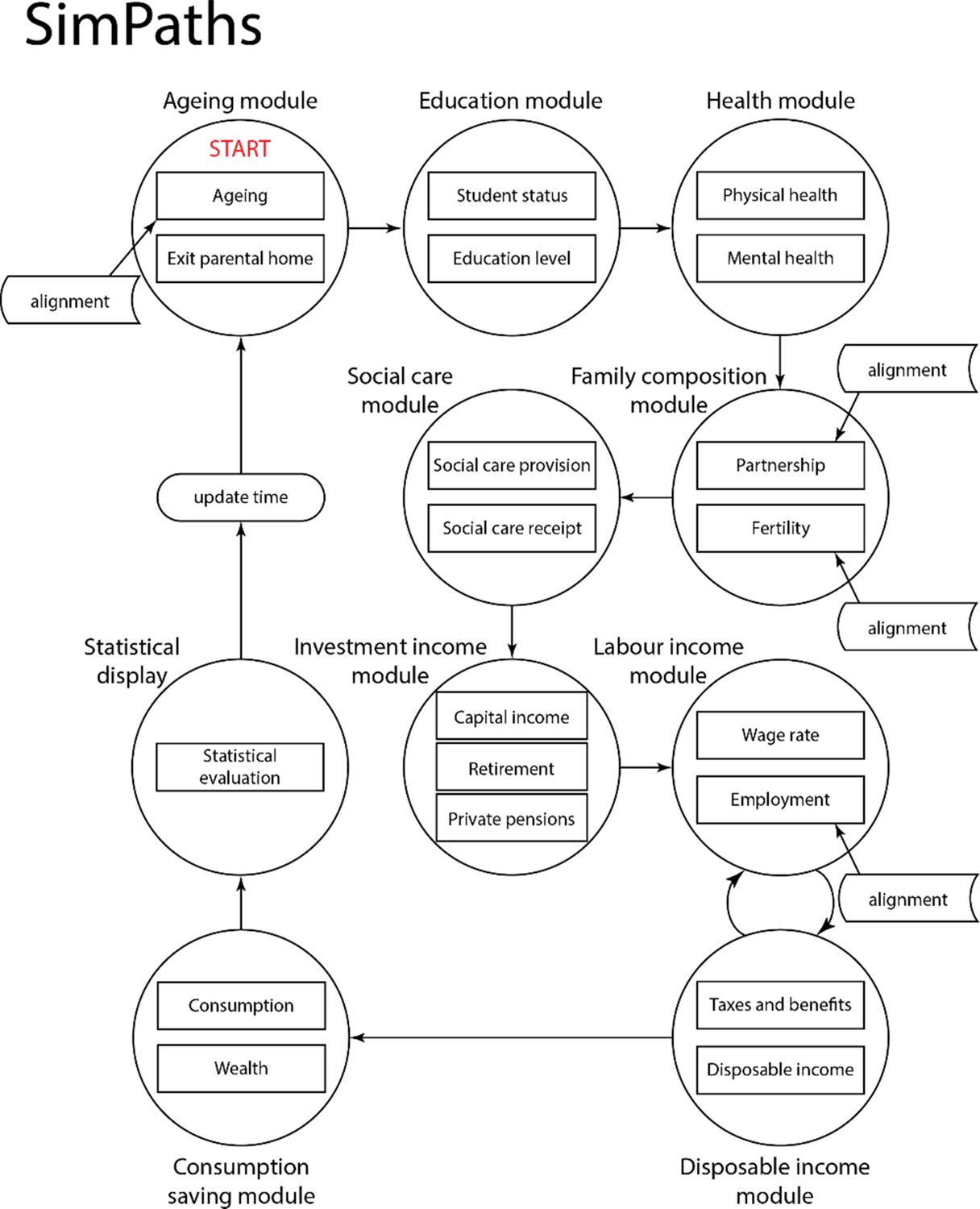
SimPaths implements an hierarchical architecture where individuals are organised in benefit units (for fiscal purposes), and benefit units are organised in households.13 The model projects data at yearly intervals, reflecting the yearly frequency of the survey data used to estimate model parameters.14 The model is composed of eleven modules: (i) Ageing, (ii) Education, (iii) Health, (iv) Family composition, (v) Social care, (vi) Investment income, (vii) Labour income, (viii) Disposable income, (ix) Consumption, (x) Health (2), and (xi) Statistical display. Variables from different modules characterise (multi-dimensional) well-being. Each module is composed of one or more processes; for example, the ageing module contains ageing, mortality, child maturation, and population alignment processes. Empirical specification of dynamic processes makes extensive use of cross-module characteristics (state variables).15
The model described in this paper is the public release 2023.12.18 of SimPaths. Simulated modules and processes are organised as displayed in Figure 1 and Table 1.
Structure and order of processes modelled in SimPaths.
List of modules and estimated processes.
| Module | Process |
|---|---|
| Ageing | Age increases. |
| Probability of leaving the parental home for those who have left education. (Students stay in the parental home). | |
| Education | Probability of remaining in education for those who have always been in education without interruptions. |
| Probability of returning to education for those who had left school. | |
| Level of education for those leaving education. | |
| Health | Self-rated health status for those in continuous education. |
| Self-rated health status for those not in continuous education (out of education or returned having left education in the past). | |
| Probability of becoming long-term sick or disabled for those not in continuous education. | |
| (Mental Health (1)) Level of psychological distress on GHQ-12 Likert scale and binary case-based indicator of psychological distress. | |
| (Mental Health (2)) Effect of exposure to employment-state transitions, household income change, and poverty for individuals aged 25 – 64 on psychological distress (GHQ-12). | |
| Family composition | Probability of entering a partnership for those in continuous education. |
| Probability of entering a partnership for those not in continuous education. | |
| Probability of partnership break-up. | |
| Probability of giving birth to a child. | |
| Social care | Probability of needing care for individuals over an age threshold. |
| Probability of receiving care for individuals under an age threshold with a disability or long-standing illness or over the age threshold, distinguished by formal, partner, son, daughter, and other providers. | |
| Hours of care for those in receipt of care, and financial cost for those receiving formal care. | |
| Probability of providing informal social care. | |
| Hours of informal social care, among those providing care. | |
| Investment income | Probability of retiring for single individuals. |
| Probability of retiring for partnered individuals. | |
| Probability of receiving capital income for those in continuous education. | |
| Probability of receiving capital income for those not in continuous education. | |
| Amount of capital income for those in continuous education. | |
| Amount of capital income for those not in continuous education. | |
| Amount of pension income for those who are retired and were not retired in the previous year. | |
| Labour income | Heckman corrected wage equation; females not employed last period. |
| Heckman corrected wage equation; males not employed last period. | |
| Heckman corrected wage equation; females employed last period. | |
| Heckman corrected wage equation; males employed last period. | |
| Hours worked, single males. | |
| Hours worked, single females. | |
| Hours worked, single male adult children. | |
| Hours worked, single female adult children. | |
| Hours worked, males with dependent partner. | |
| Hours worked, females with dependent partner. | |
| Hours worked, couples. | |
| Disposable income | Benefit recipiency indicator. |
| Amount of disposable income. | |
| Consumption & saving | Consumption. |
| Home ownership. | |
| Savings and assets. | |
| Statistical display | Evaluate summary statistics for simulated population. |
In each simulated year, agents are first subject to the ageing process, followed by population alignment. The alignment process adjusts the simulated population to match official population projections distinguished by gender, age (single-year brackets),16 and geographic region at NUTS1 level,17 which ensures that simulated output remains representative of the country’s population.
The education module determines transitions into and out of student status. Students are assumed not to work and therefore do not enter the labour supply module. Individuals who leave education have their level of education re-evaluated and can become employed.18
The health module projects an individual’s health status, comprising both self-rated general health and mental health metrics (based on a clinically validated measure of psychological distress using a Likert scale and a caseness indicator), and determines whether an individual is long-term sick or disabled (in which case, he/she is not at risk of work and may require social care).
The family composition module is the principal source of interactions between simulated agents in the model. The module projects the formation and dissolution of cohabiting relationships and fertility. Where a relationship forms, then spouses are selected via a matching process that is designed to reflect correlations between partners’ characteristics observed in survey data. The proportion of the population in a cohabiting relationship is, by default, aligned to the population aggregate in the years for which observational data is available, to account for changes in household structure introduced by the population alignment.
Females in couples can give birth to a (single) child in each simulated year, as determined by a process that depends on a range of characteristics including age and presence of children of different ages in the household. In case of divergence from the officially projected number of newborns, fertility rates are adapted by an alignment process to match population projections for new-born children distinguished by gender, region, and year.
The social care module projects provision and receipt of social care activities for people in need of help due to poor health or advanced age. The module is designed to distinguish between formal and informal social care, and the social relationships associated with informal care. The social care module accounts for the time cost incurred by care providers with respect to informal care, and the financial cost incurred by care receivers with respect to formal care.
The investment income module projects income from investment returns and (private) pensions. The approach taken to project these measures of income depends upon the model variant considered for analysis. Where consumption/savings decisions are simulated using a structural behavioural framework, then asset income is projected based on accrued asset values and exogenously projected rates of return. Alternatively, computational burden of model projections can be economised by proxying non-labour income without explicitly projecting asset holdings.
The labour income module projects potential (hourly) wage rates for each simulated adult in each year and their associated labour activity. Given potential wage rates, hours of paid employment by all adult members of a benefit unit are generated. Labour (gross) income is then determined by multiplying hours worked by the wage rate.
The disposable income module uses information concerning disability, relationship status and fertility, social care, investment income and labour income to evaluate taxes and benefits and disposable income for each projected benefit unit in each year. The model includes alternative methods for projecting employment status, some of which involve interactions between the labour income and disposable income modules to identify preferred combinations of labour supply and disposable income. An alignment routine is used to match projected rates of employment against population aggregates, to correct for biases in the labour supply model.19
Given disposable income and household demographics, the consumption module projects measures of benefit unit expenditure. Where the model projects wealth, then a simple accounting identity is used to track the evolution of benefit unit assets through time. A regression-based homeownership process predicts if the primary residence is owned by either of the responsible adults in a benefit unit, in which case the benefit unit is considered to own its home.
A secondary mental health process adjusts estimates obtained by the primary process to account for the effect of exposure to labour market transitions, such as moving in and out of employment and/or poverty.
At the end of each simulated year, SimPaths generates a series of year specific summary statistics. All of these statistics are saved for post-simulation analysis, with a subset of results also reported graphically as the simulation proceeds.
3.1. Demographics
3.1.1. Ageing
The first simulated process in each period increments the age of each simulated person by one year. Any dependent child that reaches an exogenously assumed “age of independence” (18 years-of-age in the parameterisation for the UK) is extracted from their parental benefit unit and allocated to a new benefit unit. Individuals are then subject to a risk of death, based on age, gender and year specific probabilities that are commonly reported as components of official population projections. Death is simulated at the individual level but omitting single parent benefit units (to avoid the creation of orphans).
3.1.1.1. Alignment
Population alignment is performed to adjust the number of simulated individuals to national population projections by age, gender, region, and year. Alignment proceeds from the youngest to the oldest age described by national population projections. Each age is considered in two discrete steps. First, within each age-gender-region-year subgroup, the simulated number of individuals is compared against the associated population projection. Regions with too few simulated individuals (relative to the respective target) are partitioned from those with too many. Net “domestic migration” is then projected by moving individuals from regions with too many simulated people to those with too few, until all options for (net) domestic migration are exhausted. All migratory flows are simulated at the benefit unit level, with reference to the youngest benefit unit member.
Following domestic migration, remaining disparities between simulated and target population sizes are adjusted to reflect international immigration (if the simulated population is too small), or emigration and death (if the simulated population is too large). Like domestic migration, international migration is simulated net of opposing flows and at the benefit unit level with reference to the youngest benefit unit member.20 Death is simulated in preference to international emigration for population alignment for all ages above an exogenously imposed threshold (65 for the UK).
Except for the distinction between age, gender, region, and year, all transitions simulated for population alignment are randomly distributed. This means that the model does not reflect, for example, the higher incidence of international emigration among prior international immigrants. Furthermore, the model projects international immigration by cloning existing benefit units (e.g. Duleep and Dowhan, 2008) without taking into consideration any systematic disparities between the domestic and migrant populations, including with regard to their respective financial circumstances.
3.1.2. Leaving parental home
Individuals who have recently attained the assumed age of independence and were moved to separate benefit units (see 3.1.1) are evaluated to determine if they leave their parental home. Any individual still in education is assumed to remain a member of their parental household.21 For mature children not in education, the probability of leaving their parental home is based on a probit model conditional on gender, age, level of education, lagged employment status, lagged household income quintile, region, and year (to reflect observed time trends). Mature children who are projected to remain in their parental homes may leave in any subsequent year.
3.2. Education
3.2.1. Student status
Individuals leave continuous full-time education during an exogenously assumed age band (16 to 29 for the UK). The probability of leaving continuous full-time education within this age band is described by a probit model conditional on gender, age, mother’s education level, father’s education level, region, and year.22
Individuals who are not in education may re-enter education within another exogenously assumed age band (16 to 45 for the UK). In this case, the probability of re-entering education is described by a probit model conditional on gender, age, lagged level of education, lagged employment status, lagged number of children in the household, lagged number of children aged 0-2 in the household, mother’s and father’s education levels, region, and year.
Students are considered not to work. Those who return to education can leave again in any subsequent year.
3.2.2. Educational level
Individuals who cease to be students are assigned a level of education based on an ordered probit model that conditions on gender, age, mother’s and father’s education level, region, and year. The education level of individuals who exit student status after re-entering education may remain unchanged or increase but cannot decrease.
3.3. Health
3.3.1. Physical health
Physical health status is projected on a discrete 5-point scale, designed to reflect self-reported survey responses (between “poor” and “excellent” health). Physical health dynamics are based on an ordered probit, distinguishing those still in continuous education. For continuing full-time students, the ordered probit conditions on gender, age, lagged benefit unit income quintile, lagged physical health status, region, and year. The same variables are considered for individuals who have left continuous education, with the addition of education level, lagged employment status, and lagged benefit unit composition.
3.3.2. Long-term sick and disabled
Any individual aged 16 and above who is not in continuous education can become long-term sick or disabled. The probability of being long-term sick or disabled is described by a probit equation defined with respect to lagged disability status, prevailing and lagged physical health status, gender, age, education, income quintile, and lagged family demographics.
3.3.3. Psychological distress 1 (baseline level and caseness)
In each simulation cycle, a baseline level of psychological distress for individuals aged 16 and over is determined using the 12-item General Health Questionnaire (GHQ-12). Two indicators of psychological distress are computed: a Likert score, between 0 and 36, estimated using a linear regression model; and a dichotomous indicator of the presence of potentially clinically significant common mental disorders is obtained using a logistic regression model.23 Both specifications are conditional on the lagged number of dependent children, lagged health status, lagged mental health, gender, age, level of education, household composition, region, and year.
3.3.4. Psychological distress 2 (impact of economic transitions and exposure to the Covid-19 pandemic)
The baseline measures of the level and caseness of psychological distress described above are modified by the effects of economic transitions and non-economic exposure to the Covid-19 pandemic. Fixed effects regressions are used to estimate the direct impact of transitions from employment to non-employment, non-employment to employment, non-employment to long-term non-employment, non-poverty to poverty, poverty to non-poverty, and poverty to long-term poverty, as well as changes in growth rate of household income, a decrease in household income, and non-economic effect of the exposure to Covid-19 pandemic in years 2020 and 2021. The effects of economic transitions are estimated on pre-pandemic data to ensure validity in other periods. The non-economic effects of the pandemic are estimated using a multilevel mixed-effects generalized linear model. Further details of the estimation procedure are provided in Kopasker et al. (2024).
3.4. Family composition
3.4.1. Partnerships and cohabitation
Individuals aged 18 and over who do not have a partner may decide to enter a partnership based on the outcome of a probit model. For students, the probit conditions on gender, age, lagged household income quintile, lagged number of (all) dependent children, lagged number of children aged 0-2, lagged self-rated health status, region, and year. For non-students, the probit conditions on the same set of variables as for students, expanded to include level of education and lagged employment status.
Individuals who enter a partnership are matched using either a parametric or non-parametric process, focussing exclusively on opposite-sex relationships. In the (default) parametric matching process, the model searches through the pools of males and females identified as cohabiting in each simulated period to minimise the distance between individual expectations, in terms of partner’s ideal earnings potential and age, and individual characteristics of each individual in the matching pool. The matching procedure prioritises matching individuals within regions, but if the sufficient quantity and / or quality of matches cannot be achieved, matching is performed nationally. In contrast, the non-parametric process uses an iterative proportional fitting procedure to replicate the distribution of matches observed in survey data between different types of individuals, where a type is defined as a combination of gender, region, education level, and age.
Partnership dissolution is modelled at the benefit unit level with the probability described by a probit model conditional on female partner’s age, level of education, lagged personal gross non-benefit income, lagged number of (all) children, lagged number of children aged 0-2, lagged self-rated health status, lagged level of education of the spouse, lagged self-rated health status of the spouse, lagged difference between own and spouse’s gross, non-benefit income, lagged duration of partnership in years, lagged difference between own and spouse’s age, lagged household composition, lagged own and spouse’s employment status, region, and year.
3.4.1.1. Alignment
The matching processes for new relationships outlined above fails to identify matches for all individuals flagged as entering a partnership by the related probit equations. This tends to bias the simulated population, resulting in an under-representation of partner couples. An alignment process is consequently used to match the rate of incidence of partner couples to survey targets (shares of adults in cohabiting benefit units described by annual population cross-sections reported by the Family Resources Survey, observed between 1994 and 2021). The alignment process works by adjusting the intercept of the probit relationships governing relationship formation, increasing the intercepts where the incidence of couples is too low.
3.4.2. Fertility
Females aged 18 to 44 can give birth to a child whenever they are identified in a partnership. The probability of giving birth is described by a probit model conditional on a woman’s age, benefit unit income quintile, lagged number of children, lagged number of children aged 0-2, lagged health status of the woman, lagged partnership status for those in continuous education. For those not in continuous education, the probability of giving birth is described by a probit model conditional on a woman’s age, the fertility rate of the UK population, benefit unit income quintile, lagged number of children, lagged number of children aged 0-2, lagged health status of the woman, lagged partnership status, lagged labour market activity status, level of education, and region. The inclusion of the overall fertility rate allows the model to capture fertility projections for future years, whereas the overall change in projected fertility is distributed across individuals according to their observable characteristics.
3.4.2.1. Alignment
The number of projected births is aligned to the number of newborns supplied by the official projections used for population alignment. The alignment procedure randomly samples fertile women and adjusts the outcome of the fertility process until the target number of newborns has been met.
3.5. Social care
3.5.1. Receipt of social care
The model distinguishes between individuals aged above and below an age threshold when projecting receipt of social care. This reflects the relatively high prevalence of social care received by older people, for whom more detailed information is often reported by publicly available data sources.
3.5.1.1. Receipt of social care among older people
For individuals aged above an exogenously defined threshold (65 years in the UK), the model begins by considering whether an individual is in need of care. This is simulated as a probit equation that varies by gender, education, relationship status, whether care was needed in the preceding year, self-reported health, and age. The probability of receiving care is projected using a similar set of explanatory variables. Where an individual is identified as receiving care, a multinomial logit equation is used to determine if the individual receives: i) only informal care; ii) formal and informal care; or iii) only formal care. This multinomial logit varies by education, relationship status, and age band in addition to a lag dependent variable.
For individuals projected to receive informal care, a multi-level model is used to distinguish between alternative care providers. The first level considers whether a partner provides informal care, for individuals with partners. For individuals who receive social care from their partner, the second level uses a multinomial logit to consider whether they also receive care from a daughter, a son, or someone else (other). For individuals in receipt of informal care who do not have a partner caring for them, another multinomial logit is used to select from six potential alternatives that allow for up to two carers from “daughter”, “son”, and “other”. Log-linear equations are then used to project the number of hours of care received from each identified carer. Finally, hours of formal care are converted into a cost, based on the year-specific mean hourly wages for all social care workers.
3.5.1.2. Receipt of social care among younger people
Receipt of social care among individuals under the exogenously assumed age threshold is simulated using a more stylised approach to that described for older people, reflecting the less detailed data available for parameterisation. In this case, the model focusses exclusively on informal social care for individuals simulated to be long-term sick or disabled. At the time an individual is projected to enter a disabled state, a probit equation is used to identify whether the individual receives informal social care. This identification is assumed to persist for as long as the person remains disabled.
If an individual under age 65 is identified as receiving social care, then the time of care received is described by a log-linear equation .
3.5.2. Provision of social care
The model is adapted to project provision of social care by informal sector providers; the characteristics of formal sector providers of social care are beyond the current scope of the model. The approach adopted for simulating receipt of social care described above identifies the incidence and hours of informal social care that individuals are projected to receive. In the case of people over the assumed age threshold, it also identifies the relationship between those in receipt of informal social care and their informal care providers, and the persistence of those care relationships. These details consequently provide much of the information necessary to simulate provision of informal social care, in addition to the receipt of care.
Nevertheless, the data sources for starting populations considered for SimPaths – with the notable exception of partners – generally omit social links that are implied to exist between informal social care providers and those receiving care. Specifically, links between adult children and their parents, and the wider social networks that often supply informal social care services are generally not recorded. The method that is used to project informal provision of social care is designed to accommodate limitations of the simulated data in a way that broadly reflects projection of social care receipt discussed above.
Specifically, the model distinguishes between four population subgroups with respect to provision of informal social care: (i) no provision; (ii) provision only to a partner; (iii) provision to a partner and someone else; and (iv) provision but only to non-partners. For people who are identified as supplying informal care to their partner via the process described in Section 3.5.1, a probit equation is used to distinguish between alternatives (ii: provision only to partner) and (iii: provision to a partner and someone else). Similarly, for the remainder of the population, another probit equation is used to distinguish between alternatives (i) and (iv). A log linear equation is then used to project number of hours of care provided, given the classification of who care is provided to.
3.6. Retirement
Simulation of retirement varies slightly depending on the accommodation of forward-looking expectations (see Section 3.8.2). In both cases, retirement is possible for any adult above an assumed age threshold (50 in the parametrisation for the UK). When forward-looking expectations are implicit, entry to retirement is based on a probit model that controls for gender, age, education, lagged employment status, lagged (benefit unit) income quintile, lagged disability status, indicator to distinguish individuals in excess of state pension age (accounting for changes in the state pension age), region, and year. For couples, characteristics of the spouse (employment status, reaching retirement age) also affect the probability of retirement. When forward-looking expectations are explicit, then entry to retirement is considered to be a control variable. Retired individuals may receive pension income, as described in Section 3.7.
3.7. Investment income
Investment income in SimPaths is comprised of capital income and private (non-public, personal, or occupational) pensions. The methods used to project these sources of income vary depending on whether wealth is included in the set of characteristics projected by the model. Wealth is omitted from the simulation by default but is tracked when discretionary consumption and employment decisions are simulated to reflect forward-looking behavioural incentives (described in Section 3.8.2).
3.7.1. Capital income
3.7.1.1. Wealth implicit
When wealth is not projected by the model, then the incidence of capital income among the simulated population aged 16 and over is based on probabilities described by a logit regression equation that varies by age, lagged health, lagged gross employment and capital income, region and year. For individuals not in continuous education, the list of explanatory variables for the logit equation also includes education status, lagged employment status, and lagged household composition.
For individuals simulated to be in receipt of capital income, the amount of capital income is described by linear regression models that condition on gender, age, lagged health status, lagged gross employment income, lagged capital income, region, and year for individual in continuous education. Individuals not in continuous education are also distinguished by their level of education, lagged employment status, and lagged household composition.
3.7.1.2. Wealth explicit
When wealth is explicitly projected by the model, then capital income is the product of net asset holdings and an assumed rate of return. The rate of return varies by year, and by the value of benefit unit net wealth, wi,t, as described by:
where i denotes the benefit unit and t time. denotes the (bounded) ratio of benefit unit debt to full-time potential earnings. Assuming reflects a ‘soft constraint’ where interest rates increase with indebtedness.
3.7.2. Private pensions
Private pensions are projected for adults identified as having retired in the model. The projection of retirement is described in Section 3.6.
3.7.2.1. Wealth implicit
When wealth is implicit in the model, then private pension income is projected using a linear regression model that conditions on age, level of education, lagged household composition, lagged health status, lagged private pension income, region, and year for individuals who continue in retirement. For individuals entering retirement, the probability of receiving private pension income is first determined using a logit model that conditions on having reached the state pension age, level of education, lagged employment status, lagged household composition, lagged health status, lagged hourly wage potential, region, and year. The amount of pension income is projected using a linear regression model conditional on the same observed characteristics.
3.7.2.1. Wealth explicit
When the simulation projects wealth explicitly, then an assumed fraction of benefit unit wealth at the time of retirement is converted into a life annuity, or joint-life annuity for adult couples. Annuity rates in the model are actuarily fair, given (cohort specific) mortality rates and an assumed internal rate of return.
3.8. Labour income
3.8.1. Wage rates
Hourly wage rates are simulated for each adult in the model based on Heckman-corrected regressions stratified by gender and lagged employment status (distinguishing between employed and not-employed individuals) that include as explanatory variables, part-time employment identifiers, age, education, student status, parental education, relationship status, presence of children, self-rated health, and region. For individuals observed in employment in the previous year, lagged (log) hourly wage rates are also included as an explanatory variable.
3.8.2. Employment decisions
Two alternative methods for projecting employment decisions can be considered by the model. These alternatives are both designed to reflect the influence of financial incentives on behaviour and are distinguished by whether they reflect forward-looking expectations.
3.8.2.1. Expectations implicit
The default specification of SimPaths projects labour supply using a non-forward-looking random utility model. This approach is common in the associated literature (see review by Li and O’Donoghue, 2013), and has the advantage that it limits computational burden.
The method projects labour supply as though employment decisions are made to maximise within-period benefit unit utility over a discrete set of labour/income alternatives (by default, 5 alternatives for individuals, and 25 for couples). Given any labour alternative, labour income is computed by combining hours of work with the respective hourly wage rate, projected as discussed in Section 3.8.1. The utility of the benefit unit is calculated using a quadratic utility function and takes as arguments benefit unit disposable income (see Section 3.9) and the number of hours worked by adult members.
3.8.2.2. Alignment
The estimated utility of single men, single women, and couples is adjusted to align the aggregate employment rate to the employment rate observed in the data in the validation period. The final adjustment value is used in the subsequent periods, for which no data is available. This procedure accounts for the existence of unemployment in the real economy and the fact that labour supply decisions simulated using the random utility model assume no constraints on labour demand in the economy.
3.8.2.3. Expectations explicit
The model can be directed to project labour and discretionary consumption to reflect forward-looking expectations for behavioural incentives. As for the implicit expectations case, the unit of analysis is the benefit unit. Incentives are translated into behaviour via an assumed intertemporal utility function. By default, the model adopts a nested constant elasticity of substitution (CES) utility function as described by Equation 2, although the model is designed to facilitate experimentation with alternative specifications.
where subscripts i denotes benefit unit and t time. represents within period utility derived from equivalised discretionary consumption () and time spent in leisure (). represents the warm-glow model of bequests, derived from non-negative net wealth at death (). is the expectations operator and the probability of survival of the benefit unit reference person, which varies by gender, age and year. is the coefficient of relative risk aversion, the elasticity of substitution between equivalised consumption and leisure, the utility price of leisure, and the constant exponential discount factor.
Each adult is considered to have three alternative labour supply options, corresponding to full-time, part-time and non-employment. Labour supply and discretionary consumption are projected as though they maximise the assumed utility function, subject to a hard constraint on net wealth and assumed agent expectations. Expectations are “substantively rational” in the sense that uncertainty is characterised by the random draws that underly dynamic projection of modelled characteristics. As no analytical solution to this problem exists, numerical solution methods are employed as is now standard in the dynamic programming literature (see e.g. van de Ven, 2017).
The model proceeds in two discrete steps. The first step involves solution of the lifetime decision problem for any potential combination of agent specific characteristics, with solutions stored in a look-up table. The second step uses the look-up table as the basis for projecting labour supply and discretionary consumption. Technical details of the numerical solution method are provided in the working paper version of the article (Bronka et al., 2023).
3.9. Disposable income
Disposable income is simulated by matching each simulated benefit unit in each projected period with a donor benefit unit reported by a tax-benefit reference database, following the procedure described by van de Ven et al. (2022). The database stores details of taxes and benefits alongside associated demographic and private income characteristics for a sample of benefit units. This database could be populated from a wide range of sources. The approach was originally formulated to draw upon output data derived from the UK version of EUROMOD (UKMOD), a static tax-benefit microsimulation model (see Richiardi et al., 2021), and then extended to accommodate projections from any EUROMOD country.
The matching procedure for benefit units applies coarsened exact matching over a number of discrete-valued characteristics, followed by nearest-neighbour matching on a set of continuous variables. The nearest neighbour matching is performed with respect to Mahalanobis distance measures evaluated over multiple continuous valued characteristics.
The default set of discrete value characteristics considered for matching includes age of the benefit unit reference person, relationship status, numbers of children by age, hours of work by each adult member, disability status, and informal social care provision. Similarly, the default set of continuous value matching characteristics includes original (pre-tax and benefit) income, second income (to allow for income splitting withing couples), and formal childcare costs.
Having matched a simulated benefit unit to a donor, disposable income is imputed via one of two methods. For benefit units with original income above a “poverty threshold”, disposable income is imputed by multiplying original income of the simulated benefit unit by the ratio of disposable to original income of the donor unit. For benefit units below the considered poverty threshold, disposable income is set equal to the (growth adjusted) disposable income of the donor.
Finally, adjustments to account for public subsidies for the costs of (formal) social care are evaluated separately from the database approach described above, based on internally programmed functions. This is done because public subsidies for social care are not always included in database sources (e.g. tax-benefit models) considered for analysis.
3.10. Consumption and savings
3.10.1. Non-discretionary expenditure
The model can project two forms of non-discretionary benefit unit expenditure: formal social care costs and formal childcare costs. As described in Section 3.5, social care costs are projected based on projections of hours of formal social care received and assumed hourly wage rates for social care workers.
Childcare costs are projected using a double-hurdle model, characterised by a probit function describing the incidence of formal childcare costs and a linear least-squares regression equation describing the value of childcare costs when these are incurred. Both equations include the same set of explanatory variables describing the number and age of dependent children in a benefit unit, the relationship status and employment status of adults in the benefit unit, whether any adult in the benefit unit is higher educated, region, and year.
3.10.2. Discretionary consumption
As discussed in Section 3.8.2, the model can be directed to project employment and discretionary consumption jointly to reflect forward-looking expectations for behavioural incentives. The projection of discretionary consumption varies depending on whether forward-looking expectations are chosen to be explicit or implicit within a simulation.
3.10.2.1. Expectations implicit
Yearly equivalised disposable income is calculated by adjusting disposable income (see Section 3.9) to account for benefit unit demographic composition via the modified OECD scale. Equivalised consumption is set equal to equivalised disposable income for retired individuals, and to disposable income adjusted by a fixed discount factor to account for an implicit savings rate otherwise. The assumed savings rate, in turn, influences simulated capital income (see Section 3.7.1).
3.10.2.2. Expectations explicit
As discussed in Section 3.8.2, the model evaluates solutions to the lifetime decision problem in the form of a look-up table when directed to reflect forward-looking expectations for behavioural incentives. In the case of discretionary consumption, the look-up table stores the ratio of consumption to “cash on hand”, where cash on hand is the sum of net wealth, disposable income, and available lines of credit. This ratio has the advantage that it is bounded between zero and one, which facilitates the computational routines and consideration of selected policy counterfactuals.
3.10.3. Assets accumulation
Net wealth is the key transition mechanism that balances intertemporal behavioural incentives when forward-looking expectations are treated explicitly by the model. In this case, dynamic evolution of wealth in most periods is described by the accounting identity:
where denotes the net wealth of benefit unit in period , disposable income, discretionary consumption, and non-discretionary expenditure. The only departures from Equation 5 are at the time of retirement if , when a fixed fraction of net wealth is converted into a fixed life annuity (see Section 3.7.2), or if there is a change in relationship status. In context of relationship formation, the wealth of each new partner is aggregated to obtain the wealth of the new benefit unit. In context of relationship dissolution due to separation, each spouse is assumed to take half the wealth of their preceding benefit unit. Relationship dissolution due to spouse death has no effect on benefit unit, reflecting the implicit assumption that all wealth of the deceased passes to their surviving spouse.
3.10.3.1. Home ownership
Although net wealth is not disaggregated in the model, the incidence of home ownership is reflected, as this is used as an input to for projection of psychological distress (Section 3.3.3 – 3.3.4). Home ownership is evaluated at the benefit unit level, by considering if at least one of the adult occupants is classified as a homeowner. At the individual level, home ownership is determined using a probit regression model conditional on gender, age, lagged employment status, education level, lagged self-rated health, lagged benefit unit income quintile, lagged gross personal non-employment non-benefit income, region, lagged household composition, lagged spouse’s employment status, and a time trend.
3.11. Assessing simulated uncertainty
Uncertainty regarding a model’s projections arise for a variety of reasons (Bilcke et al., 2011; Creedy et al., 2007):
Input data; due to sampling or measurement errors in initial survey populations.
Model structure;24 referring to the validity of the modelling approach adopted.
Model specification; concerning the choice of the covariates and the functional forms used, and in particular the crucial assumption that any regularity observed in the data will persist into the future.
Model parameters; concerning the statistics imprecision of parameter estimates and/or exogenously derived parameters.
Montecarlo variation; concerning sensitivity of simulated aggregates of interest to the set of random draws used to project diversity among simulated agents.
Studies based on microsimulation methods frequently ignore these sources of uncertainty, which is a recognised source of critique (e.g. Goedemé et al., 2013). This omission can generally be attributed to the observation that “the calculation of confidence intervals around model results that account for all sources of error remains a major challenge” (Mitton et al., 2000).
The first source of uncertainty listed above (i) should decline with the increasing availability of high-quality survey data, and in any case is generally beyond the scope of expertise of data analysts. Sources (ii) and (iii) that focus on model specification can be explored using established statistical techniques based on in-sample and out-of-sample measures of fit.
SimPaths accounts for parameter uncertainty (iv) by including routines that facilitate bootstrapping parameter estimates, based on estimated point values and covariance matrices. This involves repeated simulations, each based on a different random draw for model parameters. Similarly, Montecarlo variation (v) can be explored by conducting repeated simulations each based on fresh set of random draws or by arbitrarily scaling-up the simulated population size. These methods can be used to generate a distribution of model outcomes, around central projections.
4. Data, estimation and validation
4.1. Data and estimates
SimPaths uses three types of data as input:
The initial population to be evolved over time.
Donor populations used to impute the effects of tax and benefit policy.
Estimated parameters governing transition probabilities assumed by the model.
The model has been designed to draw the initial population from data reported by the UK Household Longitudinal Study (UKHLS). The UKHLS, (sometimes referred to as Understanding Society), is the successor to the British Household Panel Survey, and is the principal general-purpose panel survey administered in the UK. Multiple initial populations are derived from the UKHLS, corresponding to different years of data reported by the survey (from 2011 to 2017), and used for model validation (see below).
The donor populations for tax and benefit imputations are derived from UKMOD and are based on data reported by the Family Resources Survey (FRS). These data include a wide range of benefit unit characteristics in addition to tax and benefit payments. SimPaths imputes tax and benefit payments from these data by matching simulated individuals to individuals described by donor populations.
Parameters for the UK have been estimated on UKHLS data, Waves 1 to 8, and FRS (labour supply and social care, various years). Estimates are reported in the working paper version of the article (Bronka et al., 2023). The estimates are currently being updated to include waves 9 and 10 (up to 2019). This also involves minor changes in the specification of some of the processes.
Table 2 offers a high-level description of the specifications used in each process.
Relationship between state variables in SimPaths.
| Dependent variable | |||||||||||||||||||||
|---|---|---|---|---|---|---|---|---|---|---|---|---|---|---|---|---|---|---|---|---|---|
| Control variable | student status | education level | health status | mental health | disability status | partnership status | fertility | childcare cost | home owner | retirement status | pension income (£) | capital income (£) | low wage offer | potential wage (£) | hours worked | need social care | receive social care | type of care received | amount of care received | provide social care | amount of care provided |
| gender | c | c | c | c | c | c | c | c | c | c | c | c | c | c | c | c | c | c | c | c | |
| age | c | c | c | c | c | c | c | c | c | c | c | c | c | c | c | c | c | c | c | ||
| education | l | l | c | c | c | c,l | c | c | c | c | c | c | c | c | c | c | c | c | c | c | c |
| maternal education | c | c | l | c | |||||||||||||||||
| paternal education | c | c | c | ||||||||||||||||||
| partnership status | l | c,l | l | l | c,l | c | l | c | l | l | c | c | c | c | c | c | c | ||||
| number of children | l | l | l | l | l | l | c | l | l | l | c | ||||||||||
| age of children | l | l | l | c | |||||||||||||||||
| health status | l | l | c,l | c,l | c | l | l | l | c | c | c | c | c | c | c | ||||||
| mental health | l | ||||||||||||||||||||
| disability status | l | l | l | l | c | c | |||||||||||||||
| need social care | l | ||||||||||||||||||||
| receive social care | l | ||||||||||||||||||||
| type of care received | l | c | |||||||||||||||||||
| amount of care received | |||||||||||||||||||||
| provide social care | l | c | |||||||||||||||||||
| amount of care provided | |||||||||||||||||||||
| activity status | l | l | c,l | l | l | c | l | l | l | l | l | c | |||||||||
| hours worked | c | c,l | |||||||||||||||||||
| disposable income (£) | l | c,l | l | l | l | l | c | ||||||||||||||
| employment income (£) | l | ||||||||||||||||||||
| benefit income (£) | c | ||||||||||||||||||||
| capital income (£) | l | l | l,l2 | ||||||||||||||||||
| pension income (£) | l | l | l, l2 | l,l2 | |||||||||||||||||
| potential wage (£) | l | l | l | l | |||||||||||||||||
| home owner | c | l | |||||||||||||||||||
| region | c | c | c | c | c | c | c | c | c | c | c | c | c | c | c | c | c | c | c | c | |
| year | c | c | c | c | c | c | c | c | c | c | c | c | |||||||||
-
Note: Each column reports the controls used to update a specific individual characteristics.
The EU version of SimPaths, on the other hand, is estimated on longitudinal EU-SILC data, which is also used to build the initial population.
4.2. Validation
In this paper we report validation statistics for the workhorse version of SimPaths, parameterised to the UK. As described in Section 4 above, this version of the model uses static labour supply optimisation and includes alignment to population projections, cohabitation rates, and aggregate employment rates. The validation was undertaken by comparing simulated and observed data, starting with observations reported for 2011, and then at annual intervals to 2019. This sample window avoids complications associated with the 2008 Financial crisis on the one hand, and the Covid-19 pandemic on the other. This validation window overlaps the sample frame used to estimate model parameters (2009-2017).
Validation is always motivated by the need to increase confidence in the model (National Research Council, 2012). This, in turns, depends on the research questions that the model is designed to address, which should ultimately determine what validation tests the model has to pass. SimPaths is currently being used for a number of different research projects (see Section 5), with more applications being evaluated: a discussion of all the different research questions involved is therefore outside the scope of the present paper. Consequently, we opt here for a generic evaluation of how “realistic” the full set of model outcomes are, under a baseline parameterisation. Given the large number of state variables in the model, such a broad validation strategy spans multiple dimensions, covering both cross-sectional (evolution of summary statistics of variables over time) and longitudinal measures (transitions between states), referring both to individual variables and to their joint distribution (e.g. correlations).25 For the sake of brevity, we discuss here only a selection of cross-sectional measures, presented in graphical form for ease of visualisation, leaving validation of longitudinal measures to a future exercise. For each simulated series, 95% confidence bands are displayed, computed based on the uncertainty assessment strategy outlined in Section 3.11. The simulated confidence bands are shown against the weighted means of the corresponding variables computed on the UKHLS data.
4.2.1. Education
SimPaths reproduces the distribution of students by age accurately (Figure 2).
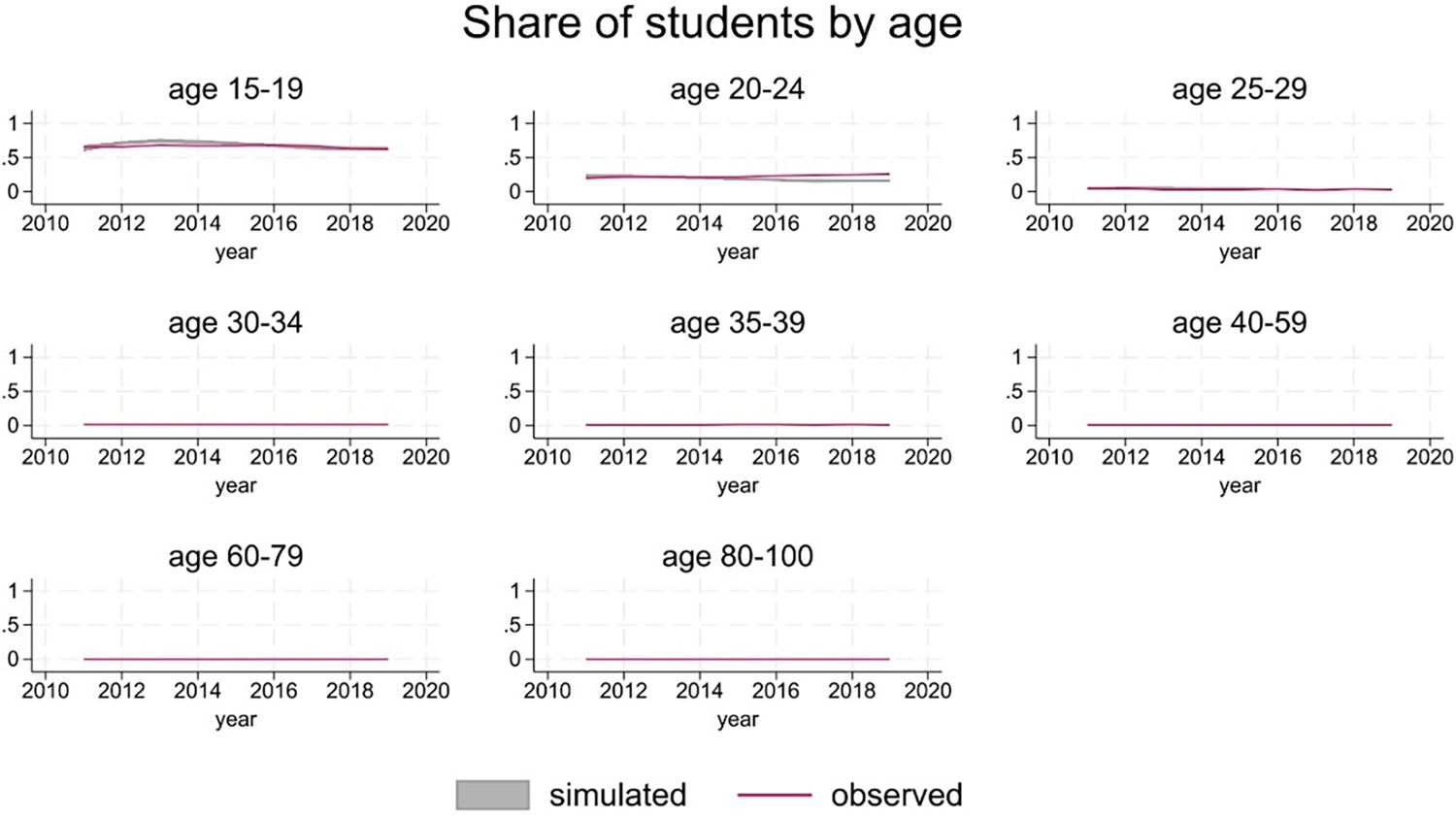
Student status.
Simulated educational attainments show convergence between the simulated and observed share of the population with high education, starting from a higher simulated level (Figure 3). This implies a slower increase than observed in the data. This is partly attributable to a conservative choice about continuation of estimated trends in the projections. More in details, specifications assume a linear time trend. This is motivated by the relatively short length of the estimation panel, which would not support a more flexible modelling of the time trend. However, extrapolating a linear trend is problematic, as it will eventually lead to implausible levels of the variable of interest. In projections, SimPaths stops the estimated linear trends after a given calendar year. The default option – adopted in this and other processes - is to stop any estimated time trend at the end of the estimation sample (2017). Data shows that the trend towards increasing educational levels is continuing beyond 2017.
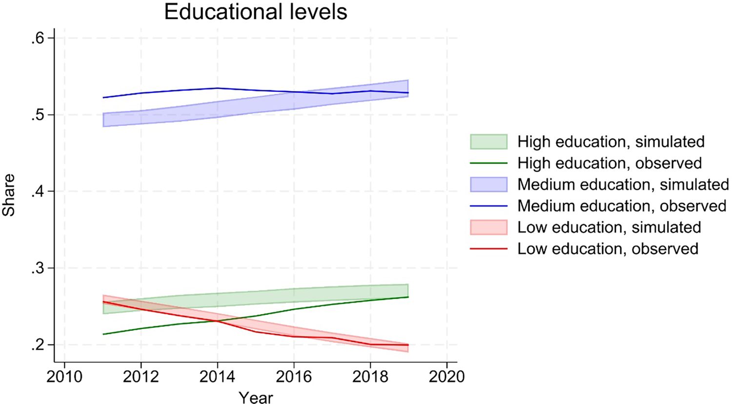
Educational attainment
4.2.2. Health
The version of SimPaths described here distinguishes between a general health score (Likert scale 1-5), and a psychological distress score (Likert scale 0-36). Projected distribution of general health by age and gender is in line with observations (Figure 4 and 5).
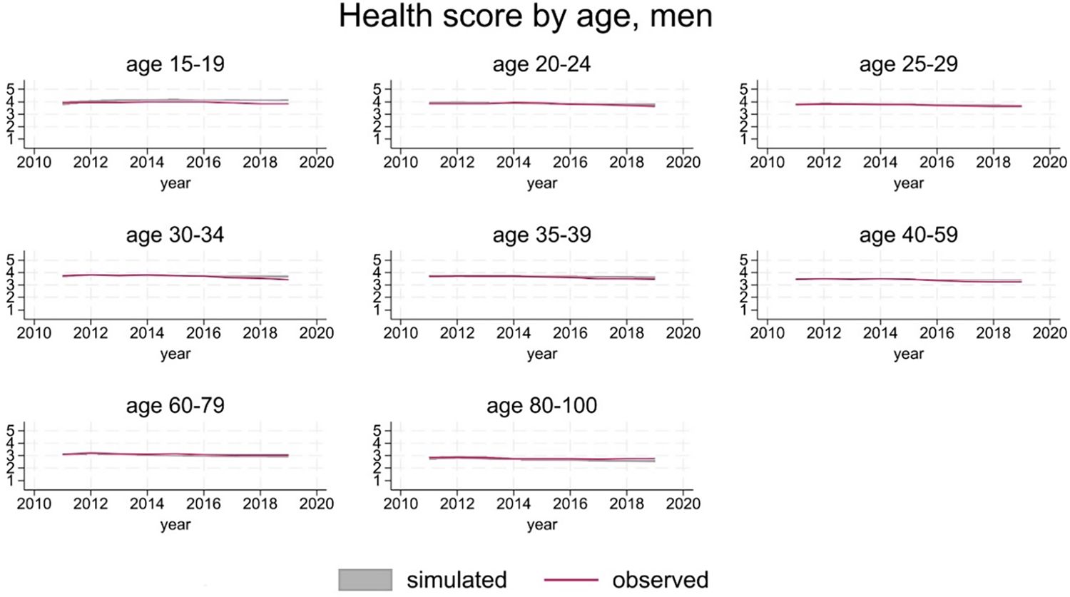
General health score, men.
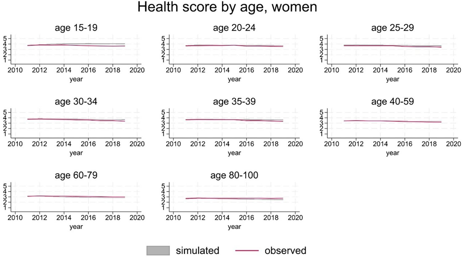
General health score, women.
For ease of interpretation, we report caseness of psychological distress (see Section 3.3.3), in addition to the score. Distributions by age and gender are substantially in line with the observations, considering the volatility implied by the level of prevalence of psychological distress in the population (Figure 6 and 7).
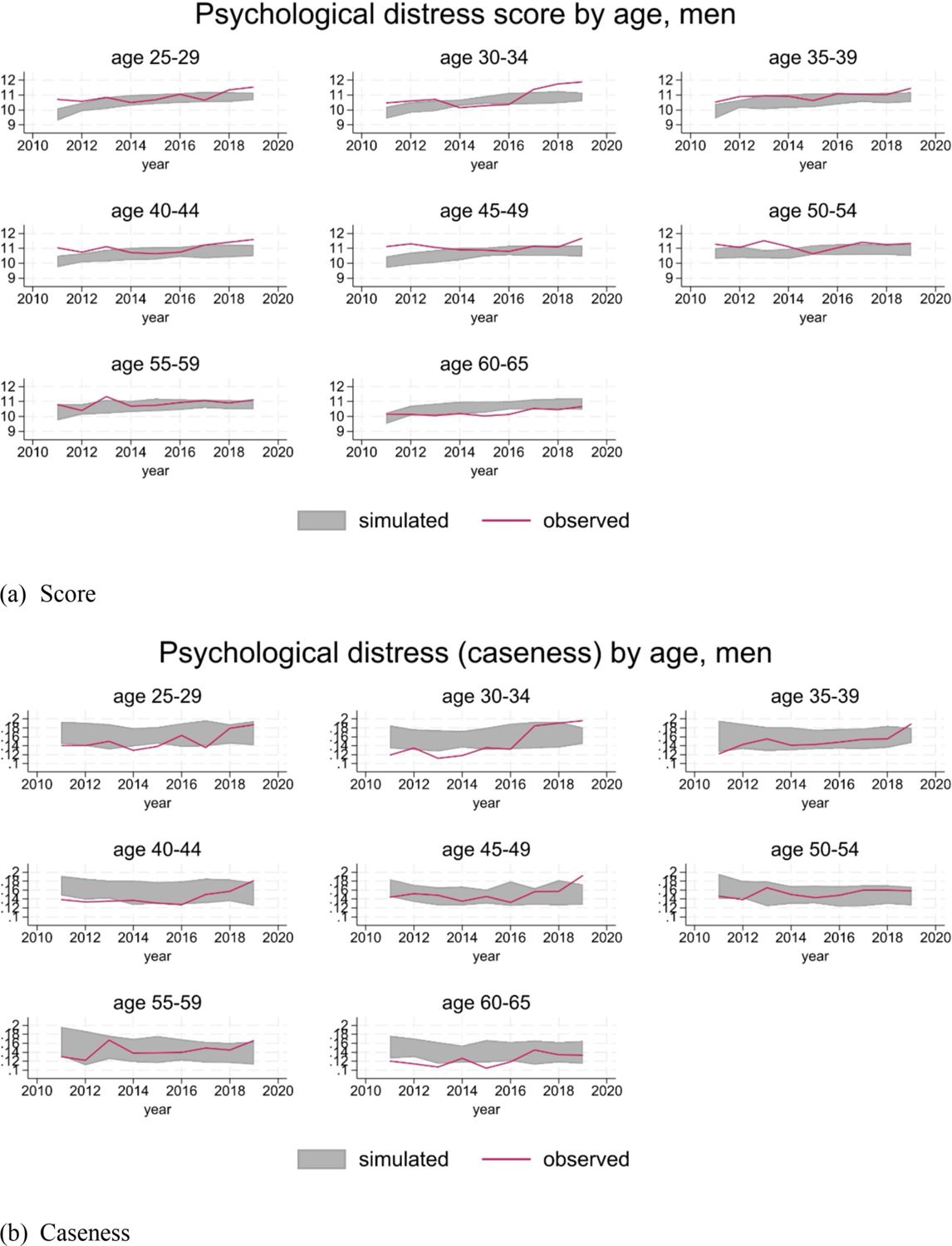
Psychological distress, men.
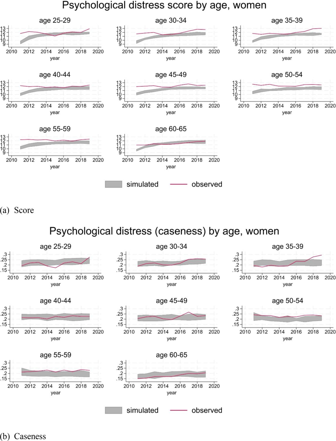
Psychological distress, women.
4.2.3. Household structure
Projections correctly reproduce a declining share of partnered households (Figure 8), although the simulated series is slightly below the observed one.
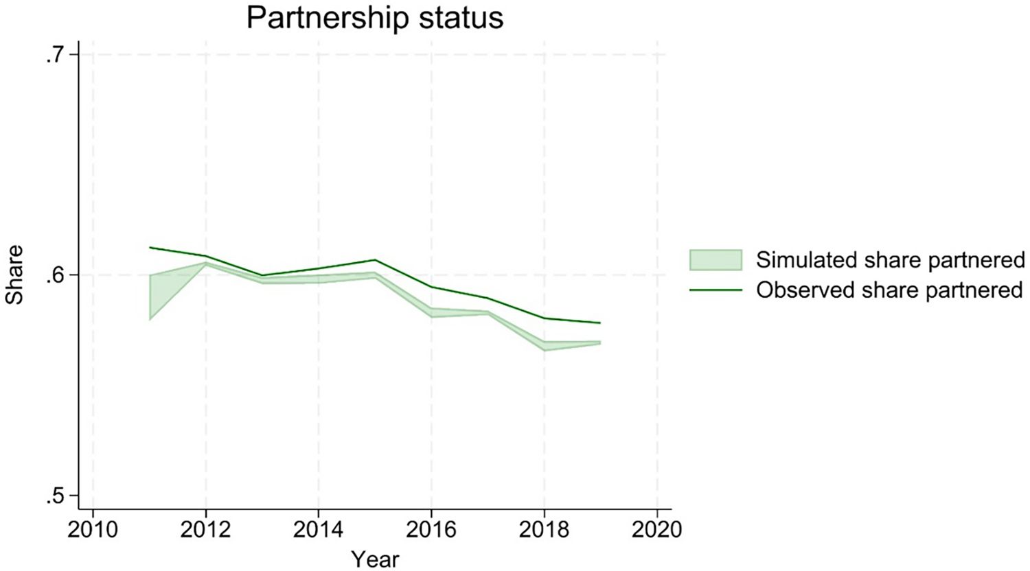
Partnership status.
The simulations also reproduce, with some approximation, the distribution of benefit units by number of children (Figure 9).
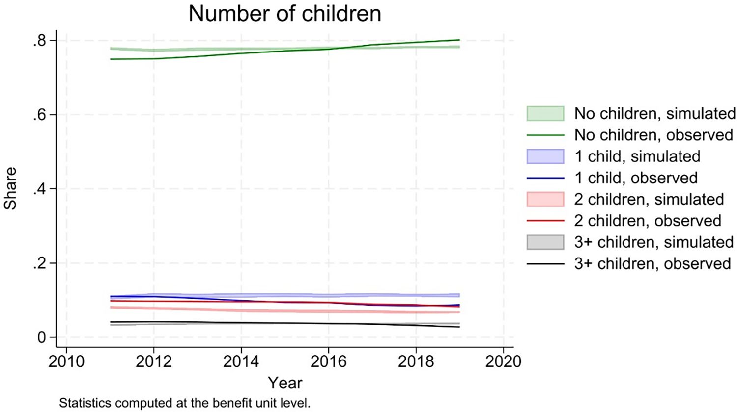
Number of children.
4.2.4. Activity status, employment and wages
As discussed above, we calibrate the labour supply model to align to observed employment rates, in the validation period. This is done by modifying the estimated parameters, rather than the simulated outcomes, resulting in a non-perfect hitting of the target. The other possible activity statuses on the other hand (in education, inactivity, retirement) are not aligned. Figure shows that the simulated activity statuses broadly follow observed data, with a slight under-projection of pensioners (see Figure 10).
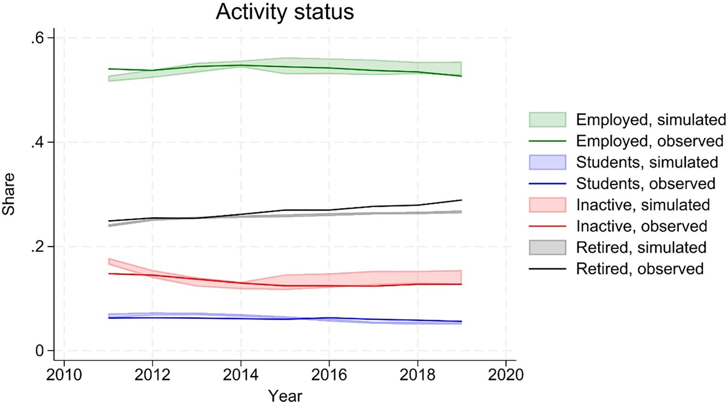
Activity status.
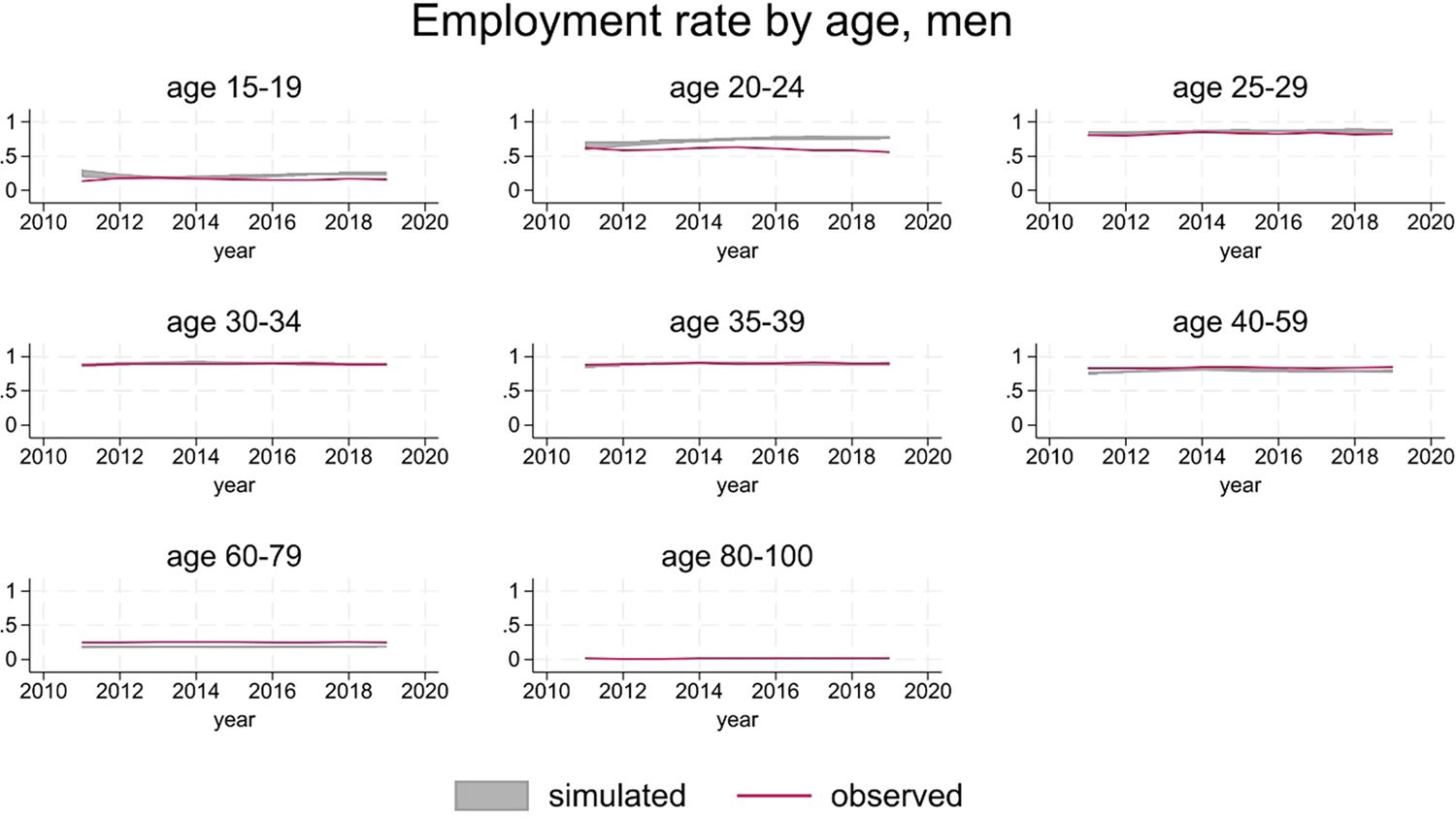
While projections are broadly aligned to aggregate employment figures, the distribution of employment by individual characteristics is freely determined by the model.
Figure 11 and 12 show that group-specific employment rates are substantially in line with the data, replicating the gender and age gradient and showing little trend over time. The main discrepancies are limited to younger men (20-24 age group), where simulations over-predict employment rates, and older women (50-59 age group), where simulations under-predict employment rates.
Employment rates, men.
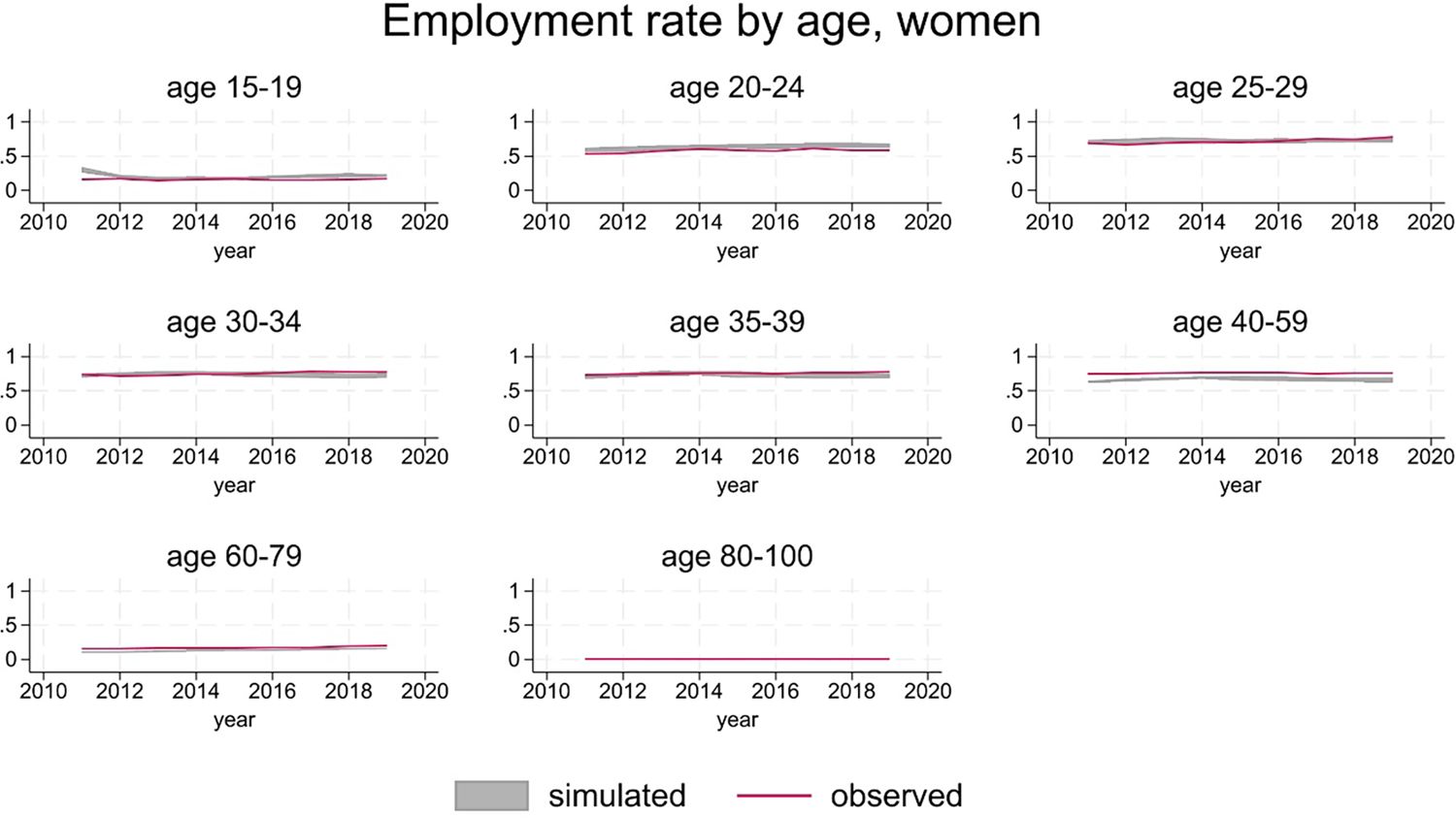
Employment rates, women.
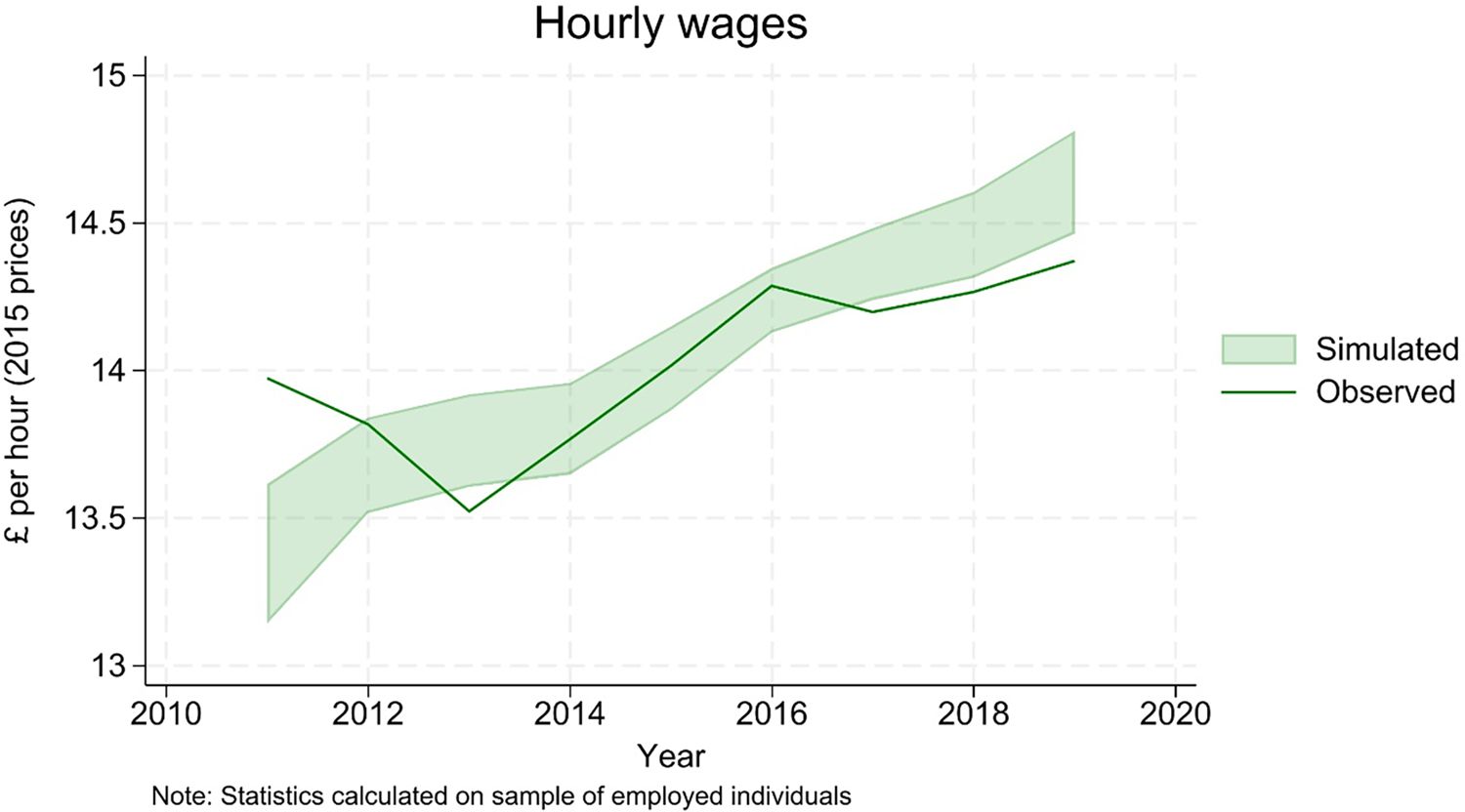
Real wages, trend.

Real wages, distribution.
Finally, the model struggles a bit in replicating the observed downward trend in hours worked (Figure 15). This is potentially due to the fact that the underlying random utility model of labour supply is estimated on one cross section of data only (2017). Sensitivity analysis shows that estimating the model on previous years results in broadly constant coefficients, which is consistent with the assumed structural nature of the model. However, the data seems to suggest that preferences might have indeed changed slightly over time.
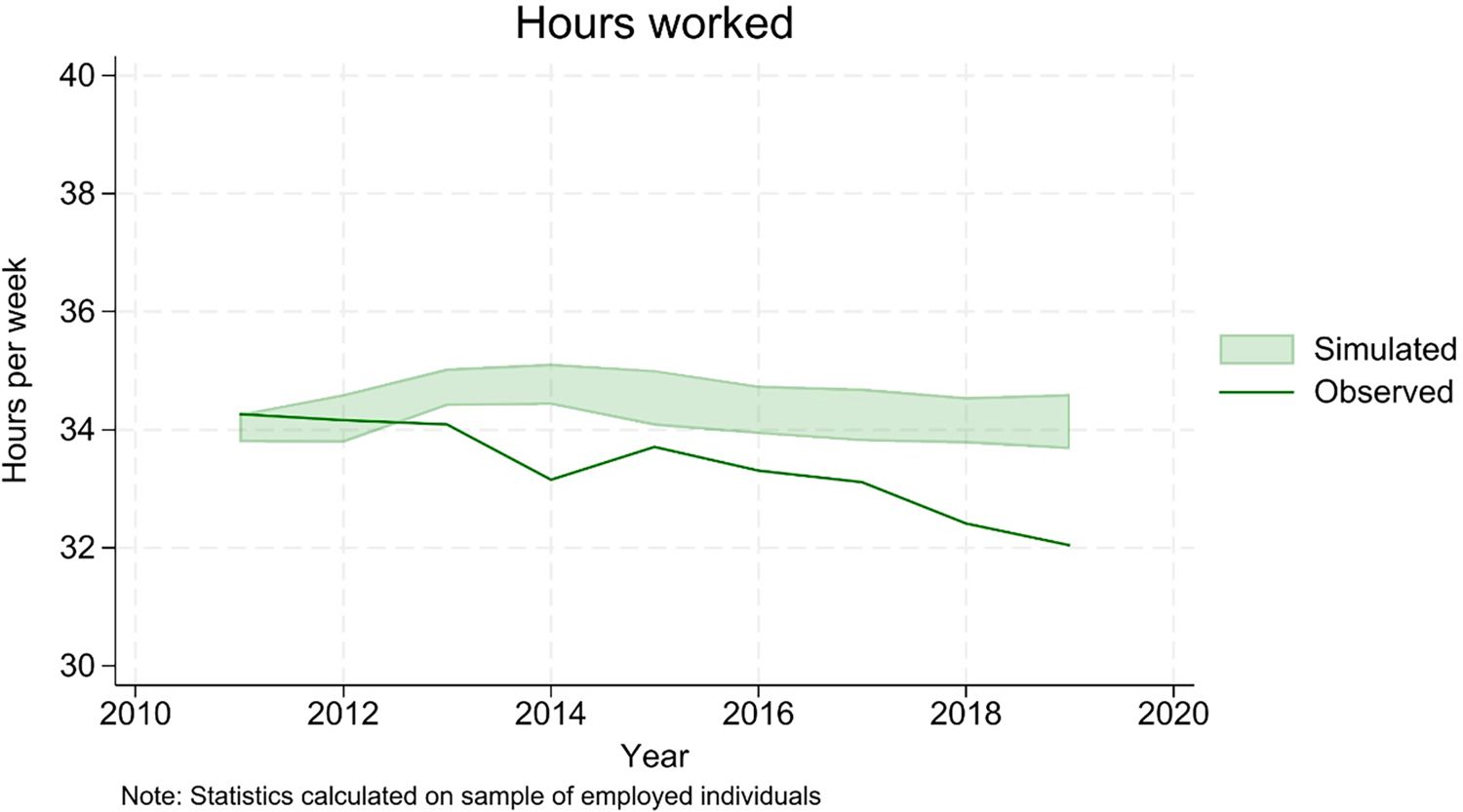
Hours worked.
4.2.5. Gross income
The model is able to replicate well both the trend and the distribution of individual gross income (Figure 16 and 17).
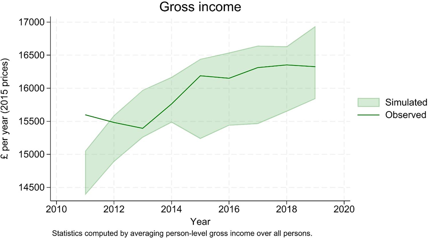
Gross income, trend.
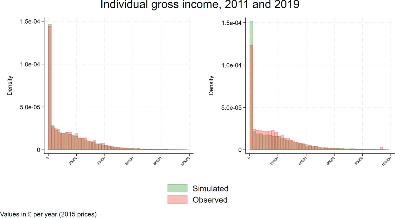
Gross income, distribution.
Projected contributions of different income sources (labour, pension, capital and miscellaneous) by age groups along the income distribution also mimic the observed ones, both in levels (Figure 18) and in shares (Figure 19).
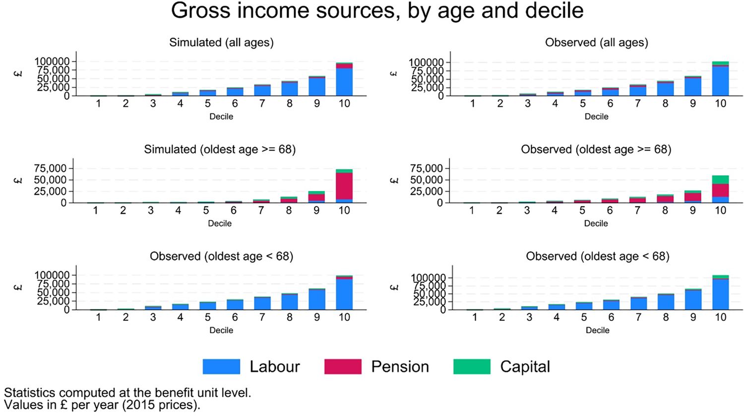
Income sources, value.
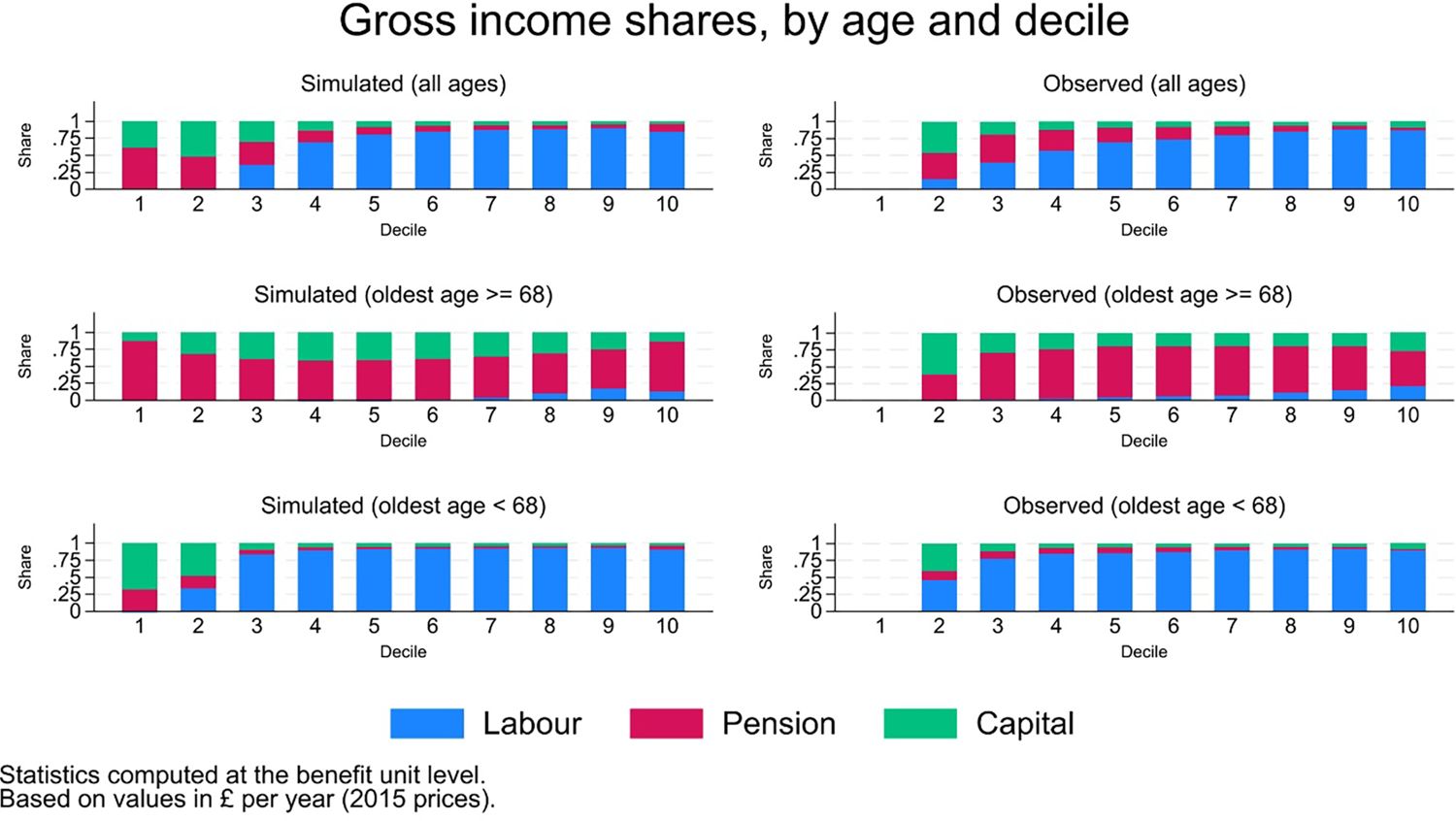
Income sources, share.
Labour income, computed by multiplying simulated hours worked by simulated wages, is obviously the main source of income for individuals below retirement age, while pension income is the main source for individuals above, on average. Both are projected with a fair level of accuracy (results not shown, but available on request). Capital income, on the other hand, is under-estimated in the simulations (average simulated values of around £1,200 - in 2015 prices - against observed values of around £1,700). However, the limited relevance of this source of income for the vast majority of the population – reflected in its small average value – limits the consequences of inadequate model specification.
4.2.6. Net income
Gross income is transformed into net income by means of the procedure described in Section 3.9. Results displayed in Figure 20 point to a slight over-estimation of disposable income (around 10%), possibly due to the fact that not all the characteristics relevant to the tax-benefit system can be simulated and controlled for in the matching procedure.26
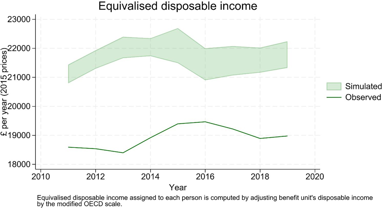
Equivalised disposable income.
The distribution of simulated disposable income however looks remarkably similar the observed one, both for the working age population, and for the population above retirement age (Figure 21).
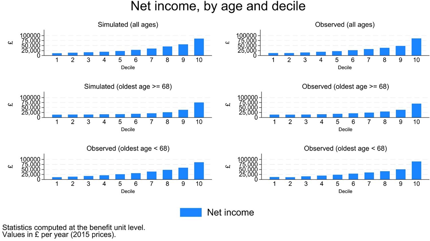
Disposable income, distribution.
4.2.7. Poverty and inequality
Biases in the simulation of disposable income translate into an under-estimation of poverty rates (Figure 22), although the error is small (around 2.5 percentage points), and the trends broadly comparable.

Poverty.
Income inequality however, as measured by percentile ratios, is very much aligned with observed measures (Figure 23).
Inequality.
4.2.8. Correlations
Maintaining the cross-sectional perspective of the previous sections, we conclude with an assessment of pairwise correlations between the main outcome variables.
Figure 24 compares simulated and observed correlation coefficients. The main features of the data are reproduced by the model, from the most trivial (positive correlation between various income measures) to less straightforward ones (positive correlation between being partnered and labour income). Health is more positively correlated with income in the simulations than in the data, possibly because we force disabled people to drop off the labour market. The negative correlation between general health and psychological distress is faithfully reproduced, as well as the very tenuous negative correlation between psychological distress and income on the one hand, and psychological distress and being partnered on the other.
Correlations.
5. Applications and extensions
Early applications of the SimPaths framework focussed on the short-to-medium term impact of social policies on mental health outcomes. Kopasker et al. (2024) consider the UK policy response to COVID-19, comparing baseline simulations with the policies that the UK government enacted in 2020-2021 to sustain incomes during the pandemic with counterfactual simulations where pre-crisis policies remained in place. Their period of analysis is 2017 to 2025. Results show that the policy response prevented a further 3.4 percentage points (pp) increase in the prevalence of common mental disorders (CMDs) with respect to pre-covid levels, on top of the more than 10pp increase observed in 2020-2021 with covid-19 legislation in place. This amounts to approximately 1.2 million additional cases of CMDs prevented by the covid-19 policy response. Beyond 2021, as employment levels rapidly recovered, psychological distress returned to the pre-pandemic trend.
Thomson et al. (2024) consider the effects of hypothetical basic income schemes over the period 2022-2026. They show that the policy has potential to improve short-term population mental health by reducing poverty, particularly among women, but impacts are highly dependent on whether individuals choose to remain in employment following its introduction. Sensitivity analysis concerning employment alternatives is conducted by replacing the labour supply module of SimPaths with alternative assumptions on the behavioural responses to the policy change.
Ongoing work investigates the employment effects and associated impact on psychological distress of the job search requirements of Universal Credit (UC), a major social protection scheme in the UK. The analysis distinguishes two channels by which conditionality affects employment outcomes. On the one hand, being on UC forces individuals to search more. On the other, the same search requirements impact mental health, reducing search effectiveness. Two more effects are identified. Individuals who are successful in their job search get a boost to their mental health associated with both entering employment and exiting UC. However, some individuals might be deterred by the search requirements from taking-up UC, resulting in reduced coverage and effectiveness of the policy. All of these effects are reinforced over time, hence requiring a dynamic analysis.
A separate analysis explores the impact of maintenance payments on mothers, fathers, and children. Both the provision and the receipt of maintenance payments impact labour supply decisions and income dynamics. These in turn affect the life course trajectories of children.
Other applications focus less on the impact of policies, and more on life course dynamics. van de Ven et al. (2024) study the individual and societal implications of increased care needs associated with population ageing over the next five decades in the UK. The analysis projects a sharp rise in the incidence of need for social care, from just under 4.0 million in 2020 to 7.6 million by 2070, with 70% of this increase driven by people aged 80 and over. The coincident costs of social care are projected to rise from £35 billion in 2020 (1.6% of GDP) to 152 billion by 2070 (2.8% of GDP), with a large fraction of this cost being sustained by depleted savings.
Informal social care provided by partners is projected to account for over half of all social care throughout the simulated time period, with the formal sector being the next largest provider accounting for approximately 15% of provisions. van de Ven et al. (2024) also compare simulations where individuals make decisions based on future expectations (the ‘expectations explicit’ approach described in Section 3) with simulations without forward looking behaviour. They show that the anticipation of the need to provide informal care leads to reduced employment and earnings. Yet the model projections suggest that precautionary savings set aside against the risk of requiring formal social care more than off-set the above factors, so that the net impact of care on savings to age 55 is positive when averaged over the population cohorts born between 1990 and 1999.
Richiardi et al. (2024) use SimPaths to explore the feedback loops between health, family and labour market outcomes, and the associated implications for income and health inequalities over alternative time horizons. They devise a computational procedure to isolate direct and indirect (mediated) effects in a microsimulation framework, consisting in artificially shocking one domain (e.g. by forcing a partnership dissolution on the simulated individuals) and comparing simulations where the impact of the shock is allowed to affect other domains (e.g. because labour market outcomes depend on, amongst other things, partnership status) with simulations where the evolution of the other domains remains unaffected and follow baseline simulations – the shock is only allowed to influence the future evolution of the shocked variable itself. Results indicate that partnership status has significant effects on other life domains, and highlight attenuation mechanisms that facilitate bouncing back to a partnered status following a union dissolution. On the other hand, health is found to have fewer connections to other life domains, with limited feedback that attenuate or exacerbate the effects of an adverse shock.
A number of ongoing funded projects provide further applications, together with the need for extending and updating the model. Major areas of development are the inclusion of measures of well-being, interaction with macro models, adoption of a spatially disaggregated synthetic population as a starting point of the simulations, and improved modelling of wealth dynamics (and associated impacts on health). The latter will distinguish between housing, pensions, other assets and unsecured debt. Private transfers between households (e.g. parents helping with the home purchase of their children) will also be included, with implications for intergenerational fairness and the intergenerational transmission of inequality. Self-rated health and psychological distress are being replaced by the physical score component (PSC) and mental score component (MCS) respectively of the SF-12 health assessment. More health outcomes are also being added, including loneliness, nutrition, and tobacco consumption. Measures of neighbourhood safety and housing quality are being introduced as pathways between socio-economic position and health outcomes. A separate workstream looks at improving modelling of external migration, which is currently treated as a residual (see Section 3.1.1). Estimates are being updated to include more recent waves of the input data, account for migrant status and ethnicity, and improve the modelling of health outcomes (including mortality). Finally, as mentioned, some of these models have already been estimated (e.g., Germany, Greece, Hungary, Italy, Poland, Spain and Sweden).
6. Funding and governance
While the open source nature of SimPaths imposes no limitation on potential users, the framework is primarily used by academic researchers. It has no institutional backing nor benefits from institutional funding. Rather, it is developed mostly through research grants. A first version of the model, then called LABSim, was developed with funding from the National Institute for the Analysis of Public Policies (INAPP), an Italian government institution (2016-2017; 2019-2022),27 building on a simpler model developed for Eurofound, the EU Agency for the improvement of living and working conditions (2015).28 The modelling framework received further funding from the UK Health Foundation (2021-2022),29 the UK National Institute for Health Research (NIHR, 2021-2028),30 the Joint Programming Initiative More Years, Better Lives (JPI MYBL, 2021-2025),31 the European Research Council (ERC, 2021-2025),32 the European Commission Horizon Europe programme (HE, 2023-2027),33 the European Spatial Planning Observation Network (ESPON, 2023-2025),34 and the Collaboration of Humanities and Social Sciences in Europe – NORFACE network (CHANSE, 2025-2028).35 The two main institutions involved in the modelling work around the SimPaths framework for the above projects are the Centre for Microsimulation and Policy Analysis (CeMPA) at the University of Essex, and the MRC/CSO Social and Public Health Sciences Unit at the University of Glasgow.
As with all open-source projects, governance presents challenges and opportunities. In terms of the six open-source governance models identified by Neary et al. (2020),36 SimPaths initially followed a Founder-leader configuration, and is now migrating towards a Self-appointing council or board structure.37 Active developers meet with a weekly frequency to coordinate project developments, and maintain single versions of the master code for the UK and the EU models respectively. “SimPaths community meetings” are held with a monthly frequency, to support adopters and users around the globe (these are mainly PhD students and policy analysts). Procedural rules are being drafted to guide contributions and ensure, as far as possible, a shared and unitary management of the project. Ultimately, the project rests on trust between developers, and on the incentives provided by the benefits of an enlarged team of developers in the context of a highly competitive funding environment.
7. Conclusion
In this paper we have introduced SimPaths, a novel dynamic microsimulation model of individual life course trajectories covering demographic, family, health and work-related events, and discussed parameterisation to the United Kingdom. The innovative features of the model lie in the flexible integration with an external tax-benefit model, and in the structural behavioural modelling at the core of individual decision making over important margins of interest. Extensive validation over the period 2011-2019 shows that the model is able to replicate well the joint evolution of individual characteristics.
SimPaths is fully open source with increasingly detailed documentation, which sets it apart from most comparable models in the existing literature. The objective of the developmental team in this regard is to facilitate, and thereby encourage researcher entry into a field that we believe presents extensive opportunities to further understanding of a wide range of practically important phenomena. From theoretical descriptions of individual decision making, sustainability of personal and public finances, and the nature of burdens and opportunities to which people are and will be subject during the prospective half century, there is much of interest to explore.
The open-source nature and governance structure of SimPaths is a radical departure from the major past and current dynamic microsimulation endeavours, which typically developed as proprietary, institutional models. While some of them passed the test of time, few have produced a consistent stream of academic outputs over the years.38 History will tell whether SimPaths will remain an ephemeral convergence of interests by a relatively small group of researchers, or will evolve into a broader research infrastructure freely available to the scientific and policy communities.
Footnotes
1.
Old-age dependency ratio (indicator).
2.
(OECD (2023), Fertility rates (indicator). Total fertility describes the number of children that would be born to each woman if she were to live to the end of her child-bearing years and give birth to children in alignment with the prevailing age-specific fertility rates.
3.
OECD (2023), Life expectancy at birth (indicator).
4.
To a different degree, this is true also for most non-OECD countries.
5.
6.
As Guy Orcutt, the father of dynamic microsimulation, put it, “I thought, ‘If you could represent a real population with a real sample, why couldn’t we represent a theoretical population with a synthetic sample? Why couldn’t we have a real sample representation of the real population at the start, and then move forward in time according to behavioral relationships applied to micro entities?’” (interview with Duo Qin, 1988, reported in Cheng, 2020).
7.
See O’Donoghue and Dekkers (2018) for a review, and O’Donoghue (2021) for an applied companion study.
8.
GENESIS: Gillman (2017). JAS-mine: Richiardi and Richardson (2017). LIAM2: de Menten et al. (2014). MODGEN: https://www.statcan.gc.ca/en/microsimulation/modgen/modgen. openM++: https://openmpp.org.
9.
10.
Statistics Canada: https://www.statcan.gc.ca/en/microsimulation/index;; Urban Institute: https://www.urban.org/research/data-methods/data-analysis/quantitative-data-analysis/microsimulation; CeMPA: www.microsimulation.ac.uk; GenIMPACT: https://www.mq.edu.au/research/research-centres-groups-and-facilities/centres/genimpact-centre-for-economic-impacts-of-genomic-medicine. For NATSEM (now defunct), see Schofield (2023). All websites accessed Dec 19, 2024.
11.
With exceptions: models are sometimes used for different applications, and small tweaks to a model often lead to related publications.
12.
The interest in life-course events is interpreted as excluding the numerous models that focus exclusively on health - for a review, see Schofield et al. (2018).
13.
A benefit unit is comprised of a single adult or adult couple and their dependent children. There can be households comprised of a single benefit unit, and benefit units comprised of a single individual. A household can be comprised of multiple benefit units only in case of adult children continuing to live at their parental home.
14.
The JAS-mine architecture also allows to introduce simulated processes cast in continuous time, where events are scheduled at precise moments in time. However, the nature of the available data sources for estimating and calibrating model parameters has thus far favoured a discrete time modelling approach, where state variables are updated at a yearly frequency. Both discrete time and continuous time processes can co-exist in JAS-mine.
15.
For example, lagged employment-related characteristics are not defined for students, but a valuable source of information for other simulated individuals.
16.
Up to age 99, and bundled together for centenarians.
17.
Ongoing work is aimed at disaggregating outcomes at NUTS3 level.
18.
Students are assumed to have a “Low” level of education until they leave school for the first time, when it is re-evaluated. Individuals who return to full time education can only improve their level of education.
19.
These might be related, for instance, by the lack of consideration of demand-side constraints in the estimation/simulation process. Employment is ultimately an equilibrium concept based on interaction between labour supply (by households) and labour demand (by firms). SimPaths however does not have a productive sector, and following a common approach in the economic literature equates labour supply with employment.
20.
That is, only immigration or emigration is projected for each population subgroup, not both.
21.
In the simulation, this is represented by a household comprised of the parental benefit unit, and one, or more, benefit units representing adult children.
22.
Conditioning on parental education introduces a correlation between socio-economic position across generations and facilitates investigation of intergenerational inequality.
23.
Individuals scoring four points or more on a 0-12 scale are classified as positive cases.
24.
Sometimes referred to as “methodological uncertainty”.
25.
Details of the process undertaken to arrive at the validation reported here are too numerous to recount succinctly, and so the current section focusses on the outcome of the process rather than the process itself, and the lessons learnt. A quick aside may, however, provide the reader with some appreciation for the issues involved. Empirical estimations of the equations that govern evolution of relationship status in the model were evaluated using pooled data from the UKHLS. From this basis, it was found that SimPaths tended to understate proportions of population projected to be in a relationship during the validation window. After further analysis, it was found that the discrepancy between the model and survey data was attributable to the interaction between the matching method used to identify partners from within the pool of simulated individuals identified as entering a relationship, and the probit relationships governing the incidence of relationship transitions. This type of mismatch reflects an issue that underlies any effort to identify parameters outside of a given model’s structure. Ideally, all model parameters should be evaluated together and endogenous to the model of interest. This is the case, for example, in related two-stage econometric methods including Simulated Minimum Distance (Lee and Ingram, 1991), Method of Simulated Moments (Stern, 1997), Indirect Estimation (Gourieroux et al., 1993), and Efficient Method of Moments (Gallant and Tauchen, 1996). In practice that is often not possible, which generates a source of model mis-identification. In the current context, an alignment method was implemented to account for the model mismatch. The alignment method adjusts the intercept of the estimated probit equations governing the incidence of entering a relationship until the model reflects summary statistics for the proportions of the population observed in survey data to be in a relationship. For years beyond the validation period, the intercept is kept constant at the last calibrated level.
26.
Figures for disposable income, where disposable income is not adjusted for the benefit unit composition, follow a similar pattern.
27.
Project “Investigating Economic Insecurity: A Microsimulation approach”.
28.
Project “Anticipating the future trend of female labour market participation and its impact on economic growth”.
29.
Project “Understanding the impacts of income and welfare policy responses to COVID-19 on inequalities in mental health: A microsimulation model”.
30.
Projects “Evaluation of the health impacts of Universal Credit: A mixed methods study”, and “The HealthMod Cluster: Enhancing Policy Modelling Capabilities to Tackle the Economic Determinants of Health and Health Inequality”.
31.
Project “Caring Over the Lifecycle: the Roles of Families and Welfare States Today and Into the Future (WELLCARE)”.
32.
Project “Health Equity of Economic Determinants (HEED): A Pan-European Microsimulation model for Health impacts of Income and Social Security Policies”.
33.
Project “Sustainable Welfare: Rethinking the roles of Family, Market and State (SUSTAINWELL)”.
34.
Project “Overlapping crises: (Re)shaping the future of regional labour markets (OVERLAP)”.
35.
Project “WELLSIM – A life course microsimulation perspective on multi-dimensional well-being in five European countries”.
36.
"Do-ocracy", Founder-leader, Self-appointing council or board, Electoral, Corporate-backed, and Foundation-backed.
37.
For a discussion of the issues involved in the governance of open-source software projects, see the special issue of the Journal of Management and Governance on “Roundtable on the Governance of Open Source Software” (Volume 11, Issue 2, May 2007), and Feller et al. (2005).
38.
An exception, albeit in the static microsimulation camp, is EUROMOD – see Sutherland (2018).
References
-
1
The dynamic cross-sectional microsimulation model MOSARTInternational Journal of Microsimulation 13:92–113.https://doi.org/10.34196/ijm.00214
-
2
Accounting for methodological, structural, and parameter uncertainty in decision-analytic models: a practical guideMedical Decision Making 31:675–692.https://doi.org/10.1177/0272989X11409240
-
3
Female Labor Supply, Human Capital, and Welfare ReformEconometrica 84:1705–1753.https://doi.org/10.3982/ECTA11576
-
4
Wages, Experience, and Training of Women over the Life CycleJournal of Labor Economics 39:S275–S315.https://doi.org/10.1086/711400
-
5
SimPaths: an open-source microsimulation model for life course analysisCeMPA WP 6/23, University of Essex.
-
6
Coping with ageing: a dynamic approach to quantify the impact of alternative policy options on future labour supply in OECD countriesCoping with ageing: a dynamic approach to quantify the impact of alternative policy options on future labour supply in OECD countries, OECD Economic Department WP 371.
-
7
Long-Term Labour Force Projections for the 25 EU Member States: A Set of Data for Assessing the Economic Impact of AgeingSSRN Electronic Journal 235.https://doi.org/10.2139/ssrn.871086
-
8
Guy H. Orcutt’s Engineering Microsimulation to Reengineer SocietyHistory of Political Economy 52:191–217.https://doi.org/10.1215/00182702-8718000
-
9
The Italian Treasury Dynamic Microsimulation Model (T-DYMM): Data, Structure and Baseline ResultsSSRN Electronic Journal 17:23–68.https://doi.org/10.2139/ssrn.4546893
-
10
Confidence intervals for policy reforms in behavioural tax microsimulation modellingBulletin of Economic Research 59:37–65.https://doi.org/10.1111/j.0307-3378.2007.00250.x
-
11
LIAM2: a New Open Source Development Tool for Discrete-Time Dynamic Microsimulation ModelsJournal of Artificial Societies and Social Simulation 17:2574.https://doi.org/10.18564/jasss.2574
- 12
-
13
The 2021 Ageing Report. Underlying Assumptions and Projection Methodology”, DG ECFINThe 2021 Ageing Report. Underlying Assumptions and Projection Methodology”, DG ECFIN, European Economy, Institutional Papers No 142.
-
14
The Dynamic Simulation of Income Model (DYNASIMThe Dynamic Simulation of Income Model (DYNASIM, Urban Institute research report.
- 15
- 16
-
17
GENESIS - The GENEric simulation system for modelling state transitionsJournal of Open Research Software 5:24.https://doi.org/10.5334/jors.179
-
18
Testing the statistical significance of microsimulation results: a pleaInternational Journal of Microsimulation 6:50–77.https://doi.org/10.34196/ijm.00088
-
19
Indirect inferenceJournal of Applied Econometrics 8:S85–S118.https://doi.org/10.1002/jae.3950080507
-
20
Challenges and opportunities of dynamic microsimulation modellingInternational Journal of Microsimulation 16:1–13.https://doi.org/10.34196/IJM.00280
-
21
Behavioral Modeling in Micro Simulation Models. A Survey”, Working Paper 1997:31, Department of Economics, Uppsala University, republished as Klevmarken, N.AInternational Journal of Microsimulation 15:78–88.
-
22
Evaluating the influence of taxation and social security policies on psychological distress: A microsimulation study of the UK during the COVID-19 economic crisisSocial Science & Medicine (1982) 351:116953.https://doi.org/10.1016/j.socscimed.2024.116953
-
23
Simulation estimation of time-series modelsJournal of Econometrics 47:197–205.https://doi.org/10.1016/0304-4076(91)90098-X
-
24
A survey of dynamic microsimulation models: uses, model structure and methodologyInternational Journal of Microsimulation 6:3–55.https://doi.org/10.34196/ijm.00082
-
25
Handbook of Microsimulation ModellingDynamic Models, Handbook of Microsimulation Modelling, Emerald Group Publishing.
-
26
IrpetDin. A Dynamic Microsimulation Model for Italy and the Region of TuscanyInternational Journal of Microsimulation 13:27–53.https://doi.org/10.34196/IJM.00224
-
27
Microsimulation Modelling for Policy AnalysisCambridge: Challenges and Innovations, Cambridge University Press.
-
28
Assessing the Reliability of Complex Models: Mathematical and Statistical Foundations of Verification, Validation, and Uncertainty QuantificationThe National Academies Press.
-
29
Understanding open source governance models, Red Hat Blog July 17https://www.redhat.com/en/blog/understanding-open-source-governance-models, Accessed, 20 December 2024.
-
30
Dynamic Microsimulation: A Methodological SurveyBrazilian Electronic Journal of Economics, 4.
-
31
Dynamic microsimulationIn: C. O’Donoghue, editors. Handbook of Microsimulation Modelling, Contributions to Economic Analysis, 293. Leeds: Emerald Group Publishing Limited. pp. 305–343.
-
32
Increasing the Impact of Dynamic Microsimulation ModellingInternational Journal of Microsimulation 11:61–96.https://doi.org/10.34196/ijm.00174
- 33
-
34
Old-age dependency ratio (indicator)https://www.oecd.org/en/data/indicators/old-age-dependency-ratio.html, Accessed, 29 March 2023.
-
35
Fertility rates (indicator)https://www.oecd.org/en/data/indicators/fertility-rates.html, Accessed, 29 March 2023.
-
36
Life expectancy at birth (indicator)https://www.oecd.org/en/data/indicators/life-expectancy-at-birth.html, Accessed, 29 March 2023.
- 37
-
38
JAS-mine: A new platform for microsimulation and agent-based modellingInternational Journal of Microsimulation 10:106–134.https://doi.org/10.34196/ijm.00151
-
39
UKMOD – A new tax-benefit model for the four nations of the UKInternational Journal of Microsimulation 14:92–101.https://doi.org/10.34196/IJM.00231
-
40
Attenuation and Reinforcement Mechanisms Over the Life CycleCeMPA WP 2/24.https://doi.org/10.2139/ssrn.4735597
-
41
Age of withdrawal from the labour force in the OECD countriesLabour Market and Social Policy Occasional Papers.
-
42
A Brief, Global History of Microsimulation Models in Health: Past Applications, Lessons Learned and Future DirectionsInternational Journal of Microsimulation 11:97–142.https://doi.org/10.34196/ijm.00175
-
43
Editorial: Special Issue in honour of Vale Emerita Professor Ann Harding AOInternational Journal of Microsimulation 16:i–iii.https://doi.org/10.34196/IJM.00278
-
44
LifeSim: A Lifecourse Dynamic Microsimulation Model of the Millennium Birth Cohort in EnglandInternational Journal of Microsimulation 14:2–42.https://doi.org/10.34196/IJM.00228
-
45
microWELT: A Dynamic Microsimulation Model for the Study of Welfare Transfer Flows in Ageing Societies from A Comparative Welfare State PerspectiveWIFO Working Papers.
-
46
Approximate Solutions to Stochastic Dynamic ProgramsEconometric Theory 13:392–405.https://doi.org/10.1017/S0266466600005867
-
47
EUROMOD: the European Union tax-benefit microsimulation modelInternational Journal of Microsimulation 6:4–26.https://doi.org/10.34196/ijm.00075
-
48
Quality Assessment of Microsimulation Models The Case of EUROMODInternational Journal of Microsimulation 11:198–223.https://doi.org/10.34196/ijm.00178
-
49
Short-term impacts of Universal Basic Income on population mental health inequalities in the UK: A microsimulation modelling studyPLOS Medicine 21:e1004358.https://doi.org/10.1371/journal.pmed.1004358
-
50
SIDD: An adaptable framework for analysing the distributional implications of policy alternatives where savings and employment decisions matterEconomic Modelling 63:161–174.https://doi.org/10.1016/j.econmod.2017.02.007
-
51
Dynamic simulation of taxes and welfare benefits by database imputationCeMPA Working Paper.
- 52
-
53
Modelling foreign labour inflows using a dynamic microsimulation model of an ageing country - SlovakiaInternational Journal of Microsimulation 13:102–113.https://doi.org/10.34196/IJM.00220
Article and author information
Author details
Srinivasa Vittal Katikireddi

Funding
Model development has been supported by the National Institute for the Analysis of Public Policies (Italy), the European Research Council (949582), the Health Foundation (2135162), the National Institute for Health and Care Research Public Health Research programme (NIHR131709), the UKRI Economic and Social Research Council (UK, grant number ES/W001543/1) and the Joint Programming Initiative (JPI More Years Better Lives), the European Union under Grant Agreement number 101095175 and the UK Government. The authors bear full responsibility for the study, including any omissions or errors made. Views and opinions expressed are however those of the author(s) only and do not necessarily reflect those of the European Union, NIHR, UKRI or the UK Department of Health and Social Care. Neither the European Union nor the UKRI can be held responsible for them.
Acknowledgements
The authors would like to thank Andy Baxter (MRC/CSO Social & Public Health Sciences Unit, University of Glasgow) for his contributions to the SimPaths project.
Publication history
- Version of Record published: April 30, 2025 (version 1)
Copyright
© 2025, Bronka, Ven, Kopasker, KatikireddiRichiardi
This article is distributed under the terms of the Creative Commons Attribution License, which permits unrestricted use and redistribution provided that the original author and source are credited.