The life-cycle income analysis model (LIAM): A study of a flexible dynamic microsimulation modelling computing framework

A dynamic microsimulation model takes individual objects (individuals, households, farms, companies) and simulates the probabilities of various events occurring at various points in time. Dynamic events may of course occur at the same point in time as other events.

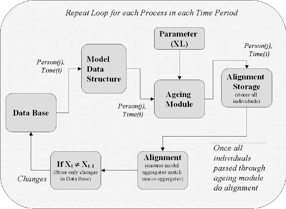
Figure 1 describes the main operations of the ageing component of the LIAM dynamic microsimulation model. In this context ‘ageing’. is a generic term covering any dynamic event that involves updating object characteristics over time. Here the operation of one particular ageing module at one point in time is examined. In reality this process occurs on a number of occasions as all the individuals in the database pass through a number of ageing modules at each point in time.

Data for each person are firstly taken from the database, having been transformed into the model data-structure, which is described in more detail below. The individual is then passed through each ageing module in turn. The ageing modules to be used are specified as part of a parameter list, which allows the order and the types of the transition processes to be varied. Input parameters for each ageing module are stored in Microsoft EXCEL spreadsheets and are accessible via the user front end. Output from each ageing module is stored, in memory, in alignment storage matrices. For example, alignment regressions produce a deterministic component XB to which is added a stochastic component, ε. These are stored in a dynamic data structure and ranked with the highest Z percent of values taken from the exogenous totals in the alignment process. If the ageing module is a transition between states, then the output will be a probability, otherwise if the ageing module is a transition between continuous amounts, for example incomes, the output is a real variable. When all individuals have been passed through the particular ageing module, alignment occurs (see section 5 below for a description). This ensures that aggregates from the micro model match macro aggregates. Finally if a variable for any individual changes then this change is registered in the database (i.e. in both the physical relational database, stored on the hard disk in ASCII and the virtual database stored in random access memory). In what follows the operations of each of these components of the ageing module are unpacked in more detail.

In this section we describe how data is handled in LIAM. We describe the database used and how data are stored within the framework. The data structure or format of the data is very important as it determines to a large extent the amount of memory required to store the data, which in turn influences the speed at which the model can run.

Figure 1

Download asset Open asset

It also has important consequences for the flexibility of the model.

Turning first to data storage, input output data are stored in ASCII format. When storing output, variables are converted from real to integer as integers require less storage space than real numbers. This is achieved by multiplying output values by 100 and truncating the result to zero decimal places. For storage we also adopt a relational database structure due to organisation and memory handling advantages.

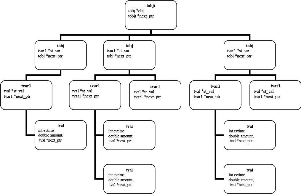
Figure 2 describes the data-structure used by LIAM. Structurally the data is stored in a hierarchy of object types (tobjt) such as person, household or firm. Each of these object types themselves consists of a number of objects (tobj) such as the actual incidence of a person or household. Events (tvar1) such as births, tenure status or identification number then occur to objects. Each event can have a number of incidences or values (tval). Within this data-structure persons are considered one set of objects and households another, with the IDs of the member individuals of a household stored as events that can happen to households. This is because persons can be members of a number of different households over time, breaking down the traditional nesting of persons with households associated with cross¬sectional data structures.

Figure 2

Download asset Open asset

We exploit the hierarchical nature of relational databases making data storage event driven. Storing model output as consecutive cross¬sections would result in severe inefficiencies, as each variable would be stored for each output period, so for example a person’s gender would be stored for each point in time. Making data storage event driven, new data is stored only when a new event occurs and thus the data changes. Gender is therefore only stored at birth. One can make significant savings in memory as a result. Each individual variable, however, requires more information than is the case in a cross-sectional data structure. For each event it is necessary to know what event occurred (tvar1), when it occurred (tval.evtime), and the value of the event (tval.amount).

There are a number of ways in which data can be stored within LIAM itself during the simulation. If the model were open, as in the case of the DEMOGEN or LifePaths models in Canada, where new spouses are generated synthetically when needed, then all of each individual’s transitions could be simulated independently of other individuals. Thus each individual could be read from the database, their life course simulated and then stored in the database one at a time. LIAM, however, uses a closed model. Except for new births or immigrants, no new individuals are generated. Marriages, for example, link individuals already in the database. This method is more straightforward to interpret as it mirrors what happens in the real world. As a result of this closed approach, individual behaviour can become dependent on the characteristics and behaviour of other members of the sample. For example, alignment to required global totals means that the chance of employment for an individual is not independent of the rest of the population, but depends upon the aggregate outcomes of the whole labour market. Other operations in the model that may depend on other individuals include the marriage market and other processes which depend on spousal information and alignment routines.

Although the model is not solely individual based (it is a multilevel model comprising Regions, Counties, Districts, Households and Persons), a side effect of the inter-person dependency engendered by the closed model approach is that it is necessary to store all individuals in memory during the simulation. To this end, therefore, during a model run the virtual database stored in memory during the operation of the program mimics the structure of the relational database stored on the hard disk. Once the data have been read from the database into memory, LIAM runs through each object type (person, family and so on), in turn simulating the life course events desired for each object of that type. Simulation processes are therefore object-type specific

Typically variables which are components of the household data structure are declared in long lists within a dynamic model. They may be initialised elsewhere and have other operations carried out in other parts of the program. As the modelling framework is so large and complicated, it rapidly becomes difficult to keep track of all the places in LIAM which need to be altered when a new variable is included. As a result, instead of declaring variables within LIAM, we declare the list of variables to be used separately in a parameter sheet (dyvardesc) .LIAM then creates space for the variable, initialises the data and carries out all necessary transformations and operations automatically. This minimises the number of model alterations necessary when a new variable is introduced, keeping the framework entirely flexible with regard to the set of variables used whilst maintaining its robustness. For example, if the user wishes to introduce a new instrument with an output variable such as health status, then the user simply needs to introduce the variable into the parameter sheet and LIAM will do the rest, without the user having to recode the framework itself. Another advantage of the flexible declaration of variables is that, because variables are stored in vectors, new composite variables can be produced easily. For example, a complex variable like disposable income, if not simulated directly, can be generated from the vector of its components such as employment income and capital income.

Another important advantage of the hierarchical method of data storage is the ease with which duration information can be accessed. As the date and value of each event is stored it is possible to determine such information as duration, duration in the last 12 months, date an event first occurred, date an event ended, duration in a particular state and so on. Information of this kind is frequently required by tax-benefit systems and other policy analysis. Additionally it is easy to access earlier values of an event such as previous earnings.

The initial database depends on the purpose of the simulation. One of the key distinctions in the literature is between longitudinal or single cohort models and population or cross-section/multi-cohort models. However, this distinction is now largely redundant due to advances in computing power. From a computing perspective, a cohort can simply be seen as an initial sample of unrelated individuals aged 0, while the population contains a sample of individuals of different ages, some of whom are related. As a result, the computing framework has been developed to handle both types of analysis. Running LIAM as a dynamic population model requires that the initial cross-section is stored in the required manner, while running the model as a dynamic cohort model requires the model to first generate an initial cohort.

The use of modularisation is an important technique that helps achieve the objectives of flexibility, transparency and robustness that LIAM requires. Modularisation means that components within the LIAM are designed to be as autonomous as possible. Modules are the components where calculations take place, each with its own parameters, variable definitions and self-contained structure, with fixed inputs and outputs. The result is a set of independent components that do not interact with each other directly, allowing the framework to operate as a collection of independent building blocks. Because each process module is entirely self contained, each can be run independently, left out or replaced by an alternative module. Constructing a program in this way allows for the model to be easily expanded to deal with new behavioural equations or functions. Also, because it allows the user to focus on individual components one at a time, without interaction with the rest of the program, the robustness of the model can be improved.

Many policy instruments depend upon multiple units of analysis. So, for example, pensions may depend upon individual characteristics such as contribution histories, age and so on, taxation may depend upon family characteristics such as both spouses’ incomes, and social protection instruments and welfare measures upon the household unit. Similarly sociological analyses and long-term care analysis may depend upon wider kinship networks. These linkages are not strictly hierarchical (e.g. region, household, family, individual). The may, in fact, consist of a web of linkages (region, firm, household, family, individual, mother, father, partner, children and so on). This multi-level structure with its complex interactions between levels is one of the main complications of microsimulation models that make it difficult to use person-based modelling frameworks. While it is not infeasible to simulate using non-hierarchical linkages such as those between relatives across households using other software packages such as social simulation and statistical packages, the non-hierarchical structure often requires one to be “creative” in designing the model due to inflexibilities in the model as they are often non-standard requirements. In contrast purpose designed microsimulation packages such as LIAM can have these data structures in-built, improving the transparency and flexibility of the modelling environment.

In the LIAM framework, the mechanism of linking objects has been automated as a relational database. Potentially any object can be linked to an object of either the same or a different object type. For example individuals of object type person (p) will be linked to their household of object type (h), while in turn the household is linked with the individuals in the household. Therefore calculation of the number of persons in a household is a process carried out at the household level. This new household level variable, npers, can be accessed by individual processes using the prefix h_npers. (The actual prefix used is user-defined.) In similar fashion linkages can be made between objects of the same type. For example a child can be linked to parent’s information, accessing mother’s education level using m_edlevel and father’s using f_edlevel.

In the initial framework, there are no predefined linkages as the objects can be of any type defined by the user. The user pre-defines all linkages using the parameterisation described below to essentially create a web of linkages between objects; essentially defining keys to link tables. As long as the nature of the linkage is defined, it is then possible at any level of the model to access information from another level. This is quite a powerful feature of the data-structure, saving both time and memory. In the absence of these linkages, such as h_npers, a new process would have to be simulated which would store this number of persons in a household as a person level variable p_hnpers (say), which is analogous to a flat file, where household level variables are stored at the person level. The use of linkages or keys provides the space saving advantages of a relational database and avoids the simulation of an extra process to convert the household variable to the person level.

While creating a new object (person, family, household, enterprise) is itself not a very complicated task, creating space and assigning initial default values, creating a new object to mimic the birth of a new person is rather more complicated. As a result we have had to develop a specific as opposed to generic new_birth function. The assignment of variable values such as single, age zero, no education and so on is straightforward. However it is also desirable that the new child inherits the linkages of the parent. So, for example, the partner (if any) of the mother at birth becomes the child’s father. Similarly other children of the mother become siblings and the hierarchical linkages such as the household, family and region of the mother are also inherited by the child.

Analogously, “killing” a person is also more difficult that killing an object. The individual needs to be extracted from the web of kinship networks and other linkages of which they form part. For example, the number of persons in a household decreases by one, whilst the spouse becomes a widow. At the same time bequest of accumulated wealth may need to be transferred and, in the case of pensions systems, contributions or entitlements may need to be transferred to surviving dependants. Again the possible complexity of the operation is far too difficult to generalise, so again object-specific routines have been required.

Migration is another complex operation. From the point of view of LIAM, emigration is analogous to killing someone. The reason for this is that, in a national model, we do not track individuals while they are abroad. (Technically, as pension rights can be accumulated overseas, one may need to simulate their life-histories while overseas, but this has been beyond the capacity of any existing model.) A variation of the pageant algorithm (Chénard, 2000) is used to ensure that the migration of family units results in national individual level aggregates being achieved.

Immigration, however, is a more difficult situation. An immigrant differs from a new birth in that they have an accumulated set of characteristics and potentially are accompanied by other family members. One solution is to simulate the range of characteristics of new immigrants on arrival. However the range of characteristics is very broad and variable and so it would be very difficult to retain the correct multi-dimensional distribution of characteristics. To avoid this problem we sample (with replacement) from a set of immigrant households in the data. Thus whenever we need an immigrant household we simply select a “real” (data-dependent) family with the actual characteristics of a new immigrant family. In addition to preserving the multi-dimensional distribution, it saves substantial computing time compared to having to simulate all of the relevant immigrant characteristics.

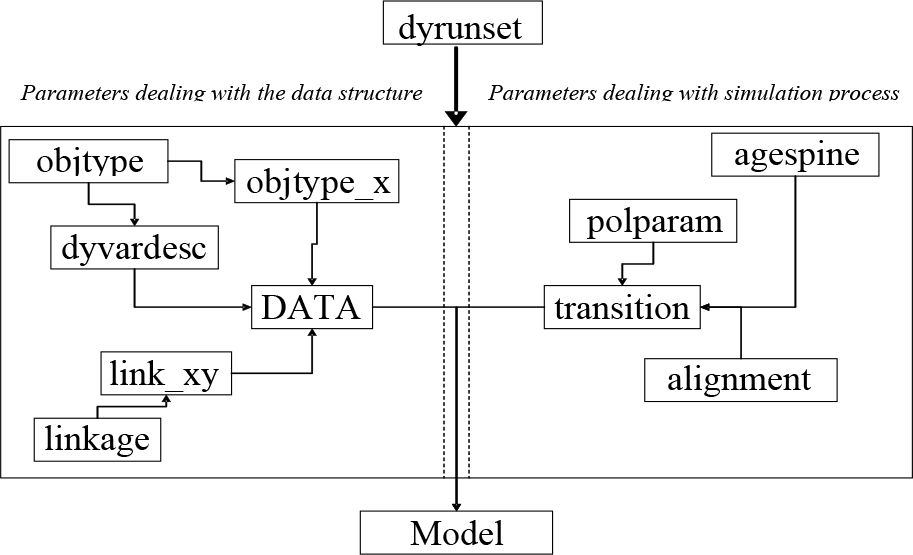
In order that modules and other components of LIAM can be changed with ease, it is necessary to store model parameters externally. Therefore, where possible, parameters are not hard coded within the framework. Figure 3 details the set of parameters used by the modelling framework. The sets of parameters, representing the flow of control in the model, are in some sense hierarchical.

Figure 3

Download asset Open asset

At the top level we have dyrunset parameters which contain the parameters necessary to run the model, detailing directories (location of input and output files), time period to be run and so on. The remaining parameters deal with either the data structure or the simulation process. Dashed lines in Figure 3 indicate this division.

On the data side the highest level parameters are contained in objtype. This file tells the model how many object types there are (region, household, person and so forth). LIAM creates each object type based upon the list defined here and assigns user-defined prefixes (for example, r,h and p). The framework then looks for files objtype_x containing the incidences of each of the object types (r, h, p), which in turn contain the identification numbers (IDs) of each object of that particular object type. So objtype_p would contain the IDs of all persons.

Related to the set of object types is a set of variables associated with each type in the dyvardesc file. In this file, all variables used in LIAM are declared and described. (In the front end, the parameter files have equivalent menus.) It is, in essence a data dictionary, for the model. This file contains information on the following attributes of each variable:

• variable name

• variable type (binary, multi-category, continuous)

• whether an income variable (monetary amount that can be added to other monetary amounts) – this prevents categorical data being summed; for example, adding gender to employment

• limits of the variable (upper and lower bounds) for debugging and validation

• whether or not a categorical variables (if so how many categories and the list of categories – for tabulation purposes),

• whether or not needs to be updated during the simulation to account for inflation

• default values to be taken by new persons

• data description (describes variable names)

Associated with each variable, there is a data table containing information about the object(s) associated with the variable (who), the time the event occurred (when) and the value of the variable (what).

While each data table within an object type is linked by the key or object ID, we need further information to link objects of the same or other type. The linkage parameters define the set of possible links between objects. The user needs to define a name for the linkage (for example, ph – person to household; hp – household to person) and the equivalent origin and destination types (p for link ph; h for link ph). These linkages between objects are stored in the linkage file link_xy. Subsequently, for each linkage listed in link_xy, LIAM pairs the relevant origin objects and destination objects (for example children to parents) and stores the resulting origin and destination IDs in a link-specific file (for example pc for children and parents).

We now consider the set of parameters that define the simulation processes. The highest level is the agespine or process spine/list. In any simulation there is an implicit ordering, and events are triggered through conditions. The process spine contains the list of modules to be run in the dynamic model, so that by varying the order of the modules and varying the content of the list, one can vary the types of processes that can be run in the model. This feature exploits the modularisation inherent in LIAM, where because each process is seen as a separate building block, the number, type and order of processes can vary without having to change the programme code. Each process or module has a corresponding parameter sheet in the parameter file “Transitions”. These parameter files tell the model the output variables of each process, the type of process, whether a process needs to be aligned and the actual process parameters themselves, such as the transition rates, regression equation and policy rules and so on. If a particular process is to be aligned, then LIAM will look for an appropriate set of alignment parameters. Sometimes individual parameters may be required to be changed between runs without any change to the set of processes. A reform to a pension simulation module where the replacement rate was changed is an example. The polparam parameter set contains information associated with each parameter for each possible “system”, where the system to be run is defined in the dyrunset parameters.

One of the most important processes in a dynamic model is the transition between different discrete states. Transition Matrices are often used to perform these operations. They specify the probability of an individual with particular circumstances moving from state A to state B. In this framework, transition matrices can be stored as log-linear models (See, for example, Dobson, 1990). In this way transition rates are decomposed into average and relative transition rates. As a result extra-relative transition rates can be added with ease. For example, if a mortality rate on average fell by 0.1% every 10 years, then a time-dependent relative probability parameter of 0.999 could be added. Similarly, this approach allows the model builder to combine information from different sources. So, for example, we combine actual age-gender specific mortality rates for 1991 taken from life-tables and use relative mortality rates taken from Nolan (1990) that incorporate socio-economic relative mortality rates.

The second type of transition process used is based upon standard regression models. At present, this type of module allows four types of dependent variable

• standard continuous dependent variable

• log dependent variable, allowing for use of the log normal distribution.

• logit discrete choice dependent variable

• probit discrete choice dependent variable

Any variable in the model can be used as a dependent variable and any variable can be used as an explanatory variable. The error term can also vary. The default error term takes a normal distribution with independent disturbances. Following Pudney (1992), LIAM also allows for the error term to be decomposed into individual specific (u_n) random effects and general error components (v_nt). However, more complicated error decompositions are also possible. This allows some degree of heterogeneity to be assigned specifically to individuals. So, for example, in determining earnings the individual specific error may represent some difference in innate ability, while the general error term represents random variation over time. Breaking up the variation in this manner will tend to reduce within lifetime variation and prevent to some degree the existence of very unusual life paths.

In the LIAM modelling framework, transitions occur at discrete time intervals because of the weakness of the data and because of the desire to be able to align the data. As Galler (1997) points out, the statistical shortcomings associated with the use of discrete time models make it is desirable to use short term discrete time periods such as a month. As the computing requirements can be substantial for monthly simulations, LIAM is sufficiently flexible to allow the user as the ability to specify the time period to be used and so monthly or annual periods can be simulated. For a fuller review of the advantages and disadvantages of continuous time versus discrete time, see O’Donoghue (2001a).

While regression models and transition matrices are stochastic processes, involving a random component, some processes are deterministic. Examples include age, which depends on the date of birth, widowhood, which depends on the death of a spouse and so on. Likewise if an individual moves from year 6 in education to year 7, years of education increase by 1.

Within the transformation-types handled by LIAM there are two types of deterministic transformation, gen and fgen. The gen functions are of simpler types, utilising calculation routines combining sets of variables using standard operations ({+,-,*,/, max,min,^,(,)}). The fgen set of functions represent ad-hoc programs. It is where we exploit, for example, the relational database structure of the data in operations such as the number of persons in a household, where the function counts the number of objects of type person linked to the object household as defined by the link_hp link file. Similarly it is where ad-hoc functions such as new_birth and killperson are defined. While gen functions and predefined fgen functions are pre-coded and parameterised so that new users can employ them, new fgen functions such as the pension system of a new country need to be programmed by the user if the existing functionality does not allow it.

If an individual is selected to marry or form a partnership a process is needed to determine which spouse they will take. The process used here is to take the characteristics of the individual chosen to marry and the characteristics of each possible spouse and determine the likelihood of a match. Similar to the method used in other models such as the CORSIM model, this is done using a logit model that estimates the probability of marriage between pairs of individuals. The parameter file therefore is identical to that used in the regression process type. The module itself forms a matrix of the characteristics of the n men and n women selected to marry. It estimates a probability for each pairing and assigns a match to the couples with the highest probability of marrying.

Bouffard et al. (2001) have identified some problematical issues associated with the marriage market, in particular with strange matches occurring amongst the last people to be married in a particular simulation. In order to avoid these issues, we allow the user to create a super-set of potential male partners, so that rather the last female in the marriage pool being forced to select an unlikely match, there remain a number of males to choose from. In addition we employ the order of Decreasing Differences algorithm proposed by Howard Redway at the UK Department for Work and Pensions, which creates a measure of the distance of an individual from the centre of the population (or the average characteristic of the population) and first selects for matching the females with the most unusual characteristics, who are likely to be the most difficult to match. The logic is that those in the centre of the data are “average people” who are more likely to find a good match than someone at the extremes.

The fourth process type is the simulation of the tax-benefit system. Re-emphasising the desire to reuse code and, wherever possible to avoid duplication, the dynamic framework has been made flexible enough to link with other specialist programs such as pre-existing tax-benefit models. As a result tax-benefit routines from other models, such as EUROMOD, can be seamlessly accessed and thus used as module components of the dynamic model.

A desirable feature often ignored in dynamic microsimulation models is the ability to include feedback loops so that behaviour can respond to changes in public policy. A criticism made by Citro and Hanushek (1997) is that dynamic models are insufficiently flexible to incorporate the demands of behavioural response. In order to be able to simulate behaviour, typically the model needs to be able to call a policy simulation routine a number of times to quantify the financial impact of alternative choices on the decision in questions such as the choice to work or retire. As a result the software framework has been designed to be able to incorporate feedback loops. The degree of modularisation that exists in the framework allows any number or order of modules to be run and for modules to be able to be run a number of times.

For example, in O’Donoghue (2001b) we implemented a simple labour supply model where labour supply depended on the tax-benefit system. In order to have labour supply depend on tax-benefit policy, the tax-benefit system needed to be run once as an input into the labour supply module and again, after labour supply has been determined, in order recalculate taxes and benefits in the light of the resulting behavioural decision. In O’Donoghue (2001b) the model used the tax-benefit system as an input into decisions to work, decisions to seek part-time employment versus full-time employment and to become self¬employed. The tax-benefit system therefore needed to be run 5 times to examine the impact of the system on the choice faced by an individual. In the case of spouses, whose behaviour can be inter-dependent, the tax-benefit system needed to be simulated 17 times (4 decisions for each spouse, plus one run on the basis of resulting joint behaviour). As a result incorporating behavioural response, although possible, can be computationally expensive.

Other possible behavioural routines that could be included are retirement decisions, consumption and benefit take-up. Although computationally expensive, the framework is sufficiently flexible should the user require and the computing power becomes available.

Finally, in order to avoid robustness problems due to modules being incorrectly specified, the model contains a debug device which ensures that all inputs required by a module are actually available (i.e. have either been generated in the model or read from the database) before each module can be run.

In discrete choice models the output for each individual is a probability. In order to use these models for predictive purposes, a decision rule is necessary. In other words, what forecasted probability (or higher) will produce an event. In order to predict a state with a logit (or probit) model, one draws a random number uniformly distributed number u_i. When

or

then a state is predicted to occur.

Another use of alignment is in correcting for predictive failures of econometric models. For example, when using discrete choice models such as logit or probit models, the predictive power is often poor. Duncan and Weeks (2000: 292) highlight that “even in functionally well-specified models, the predictive performance is poor, particularly where some states are relatively densely or sparsely represented in the data”. Greene (1997: 894) attributes this to the fact that “the maximum likelihood estimator is not chosen to maximise a fitting criterion based on prediction of y, as it is in the classical regression (which maximises R²). It is chosen to maximise the joint density of the observed dependent variable.” Thus the further the probability of an event occurring is from 0.5, the less effective these decision rules are at producing the desired result. As a result models may under or over predict the number of events. So, for example, if 5% of individuals of individuals should have the event, then the logit model may not necessarily produce 5% of events. Alignment, however, will constrain the event to occur to 5% of individuals. This is effectively a calibration mechanism and will produce the correct proportion of events. Of course, care must be in its use as alignment may lead to the disguising of errors in model specification.

The types of control totals that can be used to align to include:

• The aggregate proportion/number in a state or moving between states

• The average event value

• The distribution of values

• The average growth rate in the value of an event

In this paper we shall deal specifically only with the first type

A simple analogy for the relationship between alignment and the process modules is that the process modules, such as logit models, produce a ranking variable, while the alignment mechanism selects the number of transitions. For example, in our econometric model we may have an equation of the probability of dying as described in Equation (1), that depends on age, gender and whether an individual is disabled or not. Assuming that disabled people have a higher mortality rate, then given the same age and gender and distribution, the mortality distribution for disabled people will be higher:

The deterministic component of the model will result in those with a higher risk having a better chance of the event occurring, while the stochastic part (ξ_i) will ensure that there is some variability (so that not only those with high risk are selected). This model therefore produces the person-specific risk of dying.

In order to select the number of people that die, we use the alignment probabilities. Firstly individuals are grouped into the appropriate age and gender groups. As everyone in the relevant group will have the same age and gender, they only differ by the deterministic component for disabled people, ß₁ × Disabled_i + ß₄ × Disabled_i × Age_i, and the stochastic component ξ_i. The object then is to select to die the people in the group with the highest probabilities of dying. If B₁ is positive, proportionally more disabled will die than non-disabled. As a result we see that the output of the model equation is used to rank the individuals to whom the event occurs, but to leave the decision of experiences the event to the alignment process.

In this section we describe a practical method for ranking individuals for alignment. We take as our reference point a logistic model:

Utilising the model

will result in those with the highest risk always being selected for the event. Continuing our example above, the disabled, all other things being equal, would be selected to have a die. In reality those with the highest risk will on average be selected more than those with lower risk, rather than simply selected those with the highest risk. As a result some variability needs to be introduced.

Models based on the CORSIM framework such as the DYNACAN model (Chénard, 2000) utilise the following method. Firstly, predicted probability is produced using our econometric model:

Next, a random number, u_i, is drawn from a uniform distribution, and subtracted from the predicted probability, p*_i, to produce a ranking variable, r_i = p*_i, – u_i. This value is then used to rank individuals so that the top x% of values are selected.

A concern about this method is that the range of possible ranking values is not the same for each point. In other words, because the random number u_i, ∈ [0,1] is subtracted from the deterministically predicted p*_i, then the ranking value takes the range r_i ∈ [−1,1]. However the ranking value for each individual will only take a possible range r_i ∈ [u_r− 1, u_i]. So, for example, if p*_i is small, say = 0.1, the range of possible ranking values is [−0.9, 0.1]. At the other extreme if p*_i is large, say = 0.9, then the range of possible ranking values is [−0.1, 0.9]. Thus because there is only a small over lap for these extreme points, even if a very low random variable is selected, then an individual with a small p*_i will have a very low chance of being selected.

Ideally the range of possible ranking values should be the same, so that for each individual, r_i ∈ [a,b], with individuals with a low p*_i being clustered towards the bottom and those with a high p*_i being clustered towards the top.

We now consider an alternative method. This method takes a predicted logistic variable:

Next, a random number is drawn taken from the logistic distribution. This is added to the prediction, giving

The resulting inverse logit,

is then used to rank individuals and similarly the top x% of households are selected.

The rank produced by the two methods is not the same. The second method will be more likely to select cases at extreme points than the first, while first method will select more points with central values of p*_i.

There are a number of levels at which alignment can occur. At the lowest level, alignment refers to the decision rule used in a discrete choice model. The next level, described above in our mortality example, which is called the meso-level, concerns the idea that the aggregates for particular groups (in this case gender and age) should match desired external totals. Meso-level alignment and the use of alignment as a decision rule can however be combined into one stage.

Sometimes the desired targets are narrower than the alignment targets we use. Extending our mortality alignment example, suppose we align mortality by age, gender and occupation. We wish to include occupation in the alignment as occupational structure is very important for other characteristics in the model, and because there are known to be significant differentials in occupational mortality rates. However if one of the core targets in the model is to achieve the mortality distribution supplied by external sources such as official population projections, which may be disaggregated only by age and gender, then our meso-alignment may produce different aggregates. This will happen if our underlying occupation distribution is different to the one implicit in the official forecasts. It may therefore be desirable to adjust the results again to achieve these targets. This process is known as macro alignment. Another example follows on from the meso-alignment in the simulation of transitions between employment states. Macro alignment is then used to constrain total employment rates. See Appendix 1 for the steps involved in the macro alignment process.

Handling behavioural interactions in the model resulting from alternative scenarios is another issue one needs to consider when deciding on an alignment strategy.

One potential solution is to compare the average (pre-alignment) event value, such as the average transition rate or average earnings in the baseline scenario, with the average in the alternative scenario. One potential method is to increase alignment values by proportional difference. This is a method utilised in some dynamic models. However, this approach assumes that all processes are unconstrained. In some cases, such as mortality rates, this may be a realistic assumption. One may expect that an exogenous increase in human capital will reduce total mortality rates. In this case shifting down the alignment totals is appropriate.

Other processes face market or other institutional constraints, issues that are only partially simulated in the model. One example involves the labour market, where there is a behavioural change in labour participation in response to a tax change. If labour supply increases, then wages would fall and employment increase. This is similar to shifting the alignment probabilities. However one would have to shift earnings as well. unfortunately, due to rigidities in the labour market, this may not necessarily happen. Labour demand may be fixed, in which case we may just simply see that as more women supply labour, they simply replace people in the labour market who are less “employable”. This is similar to not shifting alignment at all. In cases where there are market interactions such as this, it may be useful to incorporate a model of the market that would inform the response of alignment totals to economic and demographic totals. At present the framework makes no explicit incorporation of behavioural change in the alignment structure. Future work on macro-micro linkages will attempt to address this.

The authors gratefully acknowledges financial assistance from the Postgraduate Fellowship of the Economic and Social Research Institute, Dublin, the Irish Department of Agriculture Rural Stimulus Fund, Center for Research on Pensions and Welfare Policies (CERP), University of Turin, the NUIG Millennium fund, the Combat Poverty Research Fund and the Targeted Socio-Economic Research programme of the European Commission (CT97-3060), the AIM project financed under the 6th Framework Research Program of the European Commission and the IDARI project financed under the 5th Framework Research Program of the European Commission. We are very grateful for the assistance of Donal Kelly, who substantially improved the code of this model. We are also grateful for comments provided by Geert Bryon, Jane Falkingham and seminar participants in LSE, Nordic Microsimulation Workshop Copenhagen, AIM workshop Madrid and colleagues in Teagasc, the DWP and NUIG. The authors remain responsible for all remaining errors.

1. Version of Record published: June 30, 2009 (version 1)

© 2009, O’Donoghue et al.

This article is distributed under the terms of the Creative Commons Attribution License, which permits unrestricted use and redistribution provided that the original author and source are credited.