Understanding low female labour force participation: Policy evaluation using microsimulation
- Institute for New Economic Thinking at the Oxford Martin School, United Kingdom
- Universita’ di Torino, and LABORatorio Revelli, Italy
- Institute for Social and Economic Research, United Kingdom
Abstract
We project medium to long term trends in labour force participation and employment for selected low-participation EU countries (Italy, Spain, Ireland, Hungary and Greece), with Sweden as a benchmark, by means of a dynamic microsimulation model. By exploring alternative scenarios to our baseline forecasts and their implications for GDP growth, we find that the gap between male and female participation is mostly explained by (i) differences in the individual conditional behaviour of older female cohorts, (ii) inadequate family policies. In particular, our results show that the conditional behaviour of younger women in the low-participation countries is similar to that in Sweden. In a nutshell, what is needed is not a change of behaviour on the side of women but a change of mentality on the side of institutions and firms.
1. Introduction
Despite recent increases in female labour market participation, the female employment rate in Europe is still 11.5 percentage points (ppt) below the employment rate of men, with huge disparities among Member States. The employment gap is highest in Italy and Greece (19.4 and 18.3 ppt respectively) and lowest in Sweden (4.6 ppt), Lithuania (2.5 ppt) and Finland (1.9 ppt). Fostering the higher participation of women is crucial to meet the Europe 2020 target of achieving an overall employment rate of at least 75% by 2020; this in turn would be crucial to reduce the risk of social exclusion and poverty for women and to achieve inclusive growth (European Comission, 2013). In this framework, Richardson et al. (2018) present medium- and long-term projections of female participation and employment rates for a selected number of EU Member States (Sweden, Italy, Spain, Ireland, Hungary and Greece) and suggest that by 2020 none of these countries except Sweden will have reached the employment rate target (though Ireland will be close). In the present paper, we analyse the role played by some key drivers (demography, education, participation behaviour) and by some policy actions in shaping future female labour market participation in the same selection of countries, in order to obtain indications on which are the factors having the highest bearing in the unsatisfactory projected evolution of participation in those countries. To be more specific, we explore the implications of different scenarios for the parameters of the microsimulation model introduced in Richardson et al. (2018), and contrast these scenarios with the baseline projections for the selected EU Member States that were also presented in that paper.
To anticipate our main conclusions, we find that the gap between male and female participation is mostly explained by (i) differences in the individual conditional behaviour of older female cohorts, (ii) inadequate family policies. In particular, our results show that the conditional behaviour of younger women in the low-participation countries is similar to that in Sweden. All this suggests that a change of behaviour on the side of women has already been achieved but it has not been accompanied by an adequate change of approach on the side of institutions and firms.
Before discussing our exercise and its results, a remark is important on the ability of the model to examine policy effects. The model on which we base our exercise is a reduced form one, estimated exploiting both within country variation and cross-sectional variation1. However, although these are reduced form equations, the inclusion of lagged values of individuals’ participation (as discussed in Section 2 below) can control for a large part of unobserved individuals’ heterogeneity as well as for persistence in individual’s behaviour. This will make the estimated parameters closer to structural ones and produce a reasonably reliable descriptive exercise about policy changes. Then the projections are made under the implicit assumption that the underlying structural relationships between variables on which the model is built will remain stable over the simulation period. They could indeed change either endogenously, because of feedback mechanisms that operate at scales not observed in the data, and therefore not considered in the model, or for exogenous reasons, because of the arrival of unexpected shocks (as a surge in migration flows) that modify both the characteristics and the behaviours of the population. Therefore, we stress that our projections should be considered as benchmarks, rather than forecasts: these benchmarks are useful insofar they point to the implicit consequences of the dynamics that are currently under way in the society, and that could trigger or require at some point in the future the activation of corrective mechanisms. Such benchmarks allow us to investigate, par différence, the effects of specific scenario or policy parameters, and the determinants of the results. This is what we do when we contrast the results obtained in the baseline scenario with those obtained under alternative scenarios. To the best of our knowledge, there is no straightforward way of improving on this. A structural labour supply model based on a tax-benefit model (EUROMOD) may be a challenging way to improve on it, and it is high on our agenda for the future. However, we reckon the present exercise interesting and informative in a descriptive – not normative – way, as it is a way of showing which determinants have the highest bearing on the dynamics of the long run trends in female participation and occupation rates.
The paper is structured as follows. In Section 2 we briefly describe the model and the baseline scenario; in Section 3 we describe the different scenarios under investigation; in Section 4 we analyse, country by country, the baseline drivers, while Section 5 is devoted to policy actions scenarios. Section 6 concludes. The Appendix reports further details on the model and the baseline scenario.
2. The model and the baseline scenario
As anticipated, the countries we analyse have been selected because they are among the most problematic in terms of female participation and employment rates, as well as in terms of gender (in)equality. Sweden has been included as a high participation benchmark. The microsimulation model is comprised of four different modules, as plotted in Figure 12: (i) Demography, (ii) Education, (iii) Household composition, and (iv) Labour market. In each period, agents first go through the Demographic module, which deals with evolving the population structure by age, gender and area, based on Eurostat official demographic projections. Then, individuals above an individual-specific age threshold retire. Retired individuals remain in the simulation until they die but nothing else happens to them, except the ageing process. Students enter the Education module. If they remain in education, nothing else happens to them until the next period. If they exit education, they join the ranks of potentially active individuals. Females enter the Household composition module, where it is determined whether they form or remain in a union and whether they give birth to a child. Then, they join males in the Labour market module, where participation and employment are finally determined.
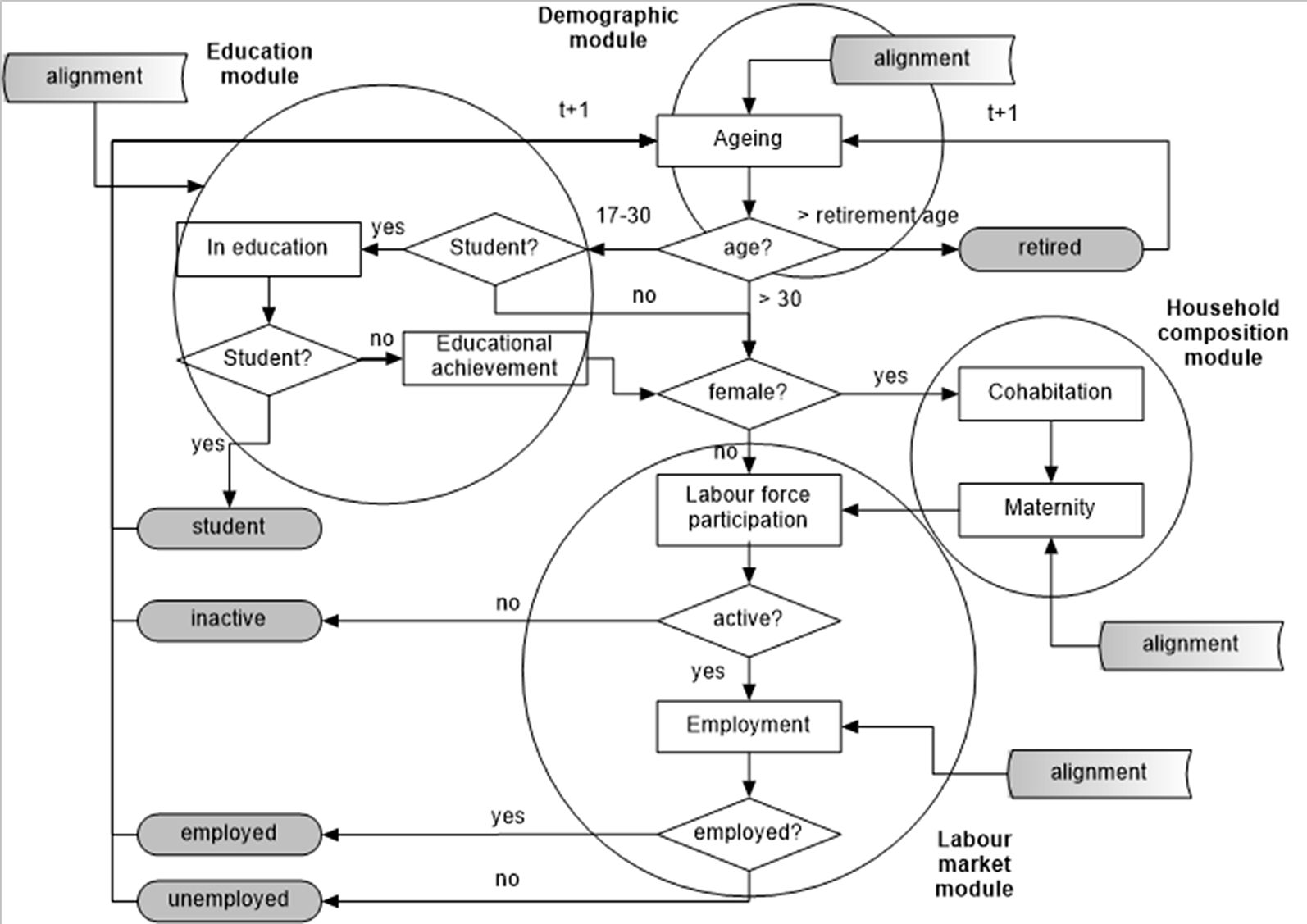

Model structure
In choosing the specifications for the different equations that contribute to determine participation patterns, we looked at the ‘usual suspects’ identified in the literature (see Del Boca and Wetzels, 2007, and Boeri et al., 2008 for surveys, but also see for instance Saurel-Cubizolles et al., 1999; Bratti et al., 2005; Attanasio et al., 2008; Genre et al., 2010; Cipollone and D’Ippoliti, 2011), as well as at policies. Thévenon (2011) performs a principal component analysis aimed at identifying the most important characteristics of family policy packages in OECD countries. He finds two main components: one related to support allowing parents to combine work with childcare, and another related to the generosity of leave entitlements in terms of money and duration. We draw from this literature, to choose the baseline scenario and the different parametrization, listed in Table 1 (policy parameters highlighted in italics)3.
Determinants of the estimated processes at an individual level. Determinants annotated with (t-1) symbolise that the one-period (one year) lag is used
| Outcome | Determinants |
|---|---|
| Student | age, gender, region |
| Education | age, gender, region |
| Consensual union (female only) | age, student(t-1), education, participation(t-1), cohabitation(t-1), children(t-1), region, retired(t-1) |
| Maternity (female only) | age, student(t-1), education, participation(t-1), cohabitation(t-1), children(t-1), region, fertility rate, public childcare, maternity benefits, part-time rate |
| Participation: women with children aged 0–3 inclusive | age, student(t-1), education, participation(t-1), cohabitation(t-1), region, public childcare, maternity benefits, part-time rate, post-crisis dummy |
| Participation: women with children aged 4–12 inclusive | age, student(t-1), education, participation(t-1), cohabitation(t-1), region, part-time rate, post-crisis dummy |
| Participation: women without children aged 0–12 inclusive | age, student(t-1), education, participation(t-1), cohabitation(t-1), region, post-crisis dummy |
| Participation: men | age, student(t-1), education, participation(t-1), region, post-crisis dummy |
| Employment | age, gender, student(t-1), education, participation(t-1), unemployment rate, region, post-crisis dummy |
Although these are reduced form equations, the inclusion of lagged values of individuals’ participation can control for a large part of unobserved individuals’ heterogeneity as well as for persistence in individual’s behaviour. This will make the estimated parameters closer to structural ones and produce a reasonably reliable descriptive exercise about policy changes.
As a final remark, notice that employment rates are computed in the microsimulation conditional on participation and do not feed back into the evolution of the other variables. I.e., differences in employment rates are entirely explained by differences in participation rates, for given parameters controlling the speed of recovery from the Great Recession.4 Hence, in presenting the results we will focus mainly on participation rates; employment rates will be discussed for the scenarios involving a change in parameters related to the recovery from the Great Recession only.
Participation rates projected according to the baseline scenario will be plotted in the result sections 4 and 5, along with the participation rates projected according to the different scenarios discussed in the next section.
3. The alternative scenarios
They are chosen with two objectives in mind. First, we wish to offer a better comprehension of the drivers of the baseline results, by deliberately “switching off” country-specific differences one at a time. Hence, we analyse what happens in the low participation countries (Italy, Spain, Greece, Hungary and Ireland) when we endow them with ‘Swedish features’, from demographic evolution, to educational attainments and conditional participation behaviour of women. Second, we wish to investigate the effects of key parameters which might be affected by policies. These involve the speed of recovery from the Great Recession, the suppression of early retirement opportunities, and more favourable family policies.
We will label the two sets of different parameterisations baseline drivers and policy actions, respectively, though the distinction between the two sets is fuzzy and mainly concerns the choice of the parameters values: when analysing the baseline drivers, we set the relevant parameters to “extreme” values (those of the benchmark country, which are generally implausible for the other countries), while when we investigate policy actions we choose “reasonable” values for the parameters. This because we acknowledge that policies might also affect the baseline drivers – for instance, by modifying the incentives that shape fertility rates, migration flows, or educational choices. To address this issue, starting from the “extreme” Swedish values for – e.g. – educational attainments, we elaborate on the responsiveness of the model outcomes with respect to more “reasonable” educational levels, in order to provide an idea of the effects of more realistic educational policies.
Notice that, when analysing baseline drivers we are not in the position to decompose exactly the total projected change in participation and employment rates into their different causal pathways, as changing parameters in turns, as described, prevents us to compute exact shares of the differences in outcomes between the low participation countries and Sweden, as they do not sum up mechanically to one. To do so we would have needed an Oaxaca-Blinder decomposition exercise, but the cost of doing so would have been to prevent us to analyse the impact of these differences in the model projections. However, in pursuing our strategy, we can nevertheless provide an intuitive way of discriminating between more and less important channels, focussing on the relative size of these differences.
3.1. Baseline drivers
3.1.1 Swedish participation
The Swedish participation scenario is meant to disentangle the effects of individual characteristics from composition effects, in explaining participation rates. For instance, having small children negatively affects female participation, to a degree which is estimated in the data and is country-specific. The (country-specific) estimated coefficients measure the effects of the covariates (having versus not having small children in our example) on the outcome.5 On top of the differences in the estimated coefficients, countries also differ with respect to the fraction of women with small children, and in their characteristics (age, education, etc.), that is in the composition of the population with respect to the determinants of the outcome of interest. The Swedish participation scenario assumes that in all countries, all covariates have the same effect as in Sweden, with respect to participation. Hence, differences in outcomes must be attributed to composition effects only. While in the Swedish demography and the Swedish education scenarios described below we keep population characteristics fixed to Swedish levels, here we keep their effects fixed to Swedish levels, and keep the country-specific population characteristics as in the baseline.6 Hence the Swedish participation scenario allows us to answer the following questions: What would happen in country X if individuals were to behave as in Sweden, with respect to their labour force participation decisions? Is it behaviour (conditional on characteristics), or is it the characteristics of the population in terms of the distribution of individual traits, that matters the most in explaining the outcome?7
3.1.2. Swedish demography
In the Swedish demography scenario, the demographic evolution is the same as in Sweden8. Table 2 reports the projected evolution of the old-age dependency ratio (the ratio between the projected number of persons aged over 65 years and the projected number of persons aged between 15 and 64 years, expressed per 100 persons aged 15–64 years) in the baseline scenario, ordered from lowest (Ireland) to highest (Italy) in 2015. Sweden is the country which is closest to a demographic equilibrium, with an old-age dependency ratio that is projected to grow only moderately over the forecasting horizon: from being in the middle of the ranking in 2015, it is expected to become the country with the lowest ratio among the selected countries from 2040 onwards. This reinforces the choice of Sweden as a benchmark.
Projected old-age dependency ratio, baseline scenario
| Old-age dependency rates (%) | |||||
|---|---|---|---|---|---|
| Year | 2015 | 2020 | 2030 | 2040 | 2050 |
| Ireland | 19.8 | 23.2 | 30.3 | 38.6 | 44.8 |
| Hungary | 26.4 | 30.5 | 34.4 | 39.8 | 47.3 |
| Spain | 27.8 | 30.4 | 39.6 | 53.5 | 62.5 |
| Sweden | 31.2 | 33.0 | 35.5 | 37.4 | 37.5 |
| Greece | 31.9 | 34.3 | 41.2 | 53.2 | 63.6 |
| Italy | 33.3 | 34.9 | 40.8 | 49.9 | 52.9 |
-
Source: Eurostat – Population Projections EUROPOP2013.
3.1.3. Swedish education
In the Swedish education scenario, the distribution of educational attainments is the same as in Sweden. Table 3 reports the share of individuals with respectively high and low levels of education, in the baseline scenario, in the base year of the simulation. Sweden is the country with the highest (lowest) proportion of people with high (low) education. In the Swedish education scenario, initial educational attainments are modified to reflect the same distribution of educational levels as in Sweden. Then, the share of highly educated individuals increases, in all countries, as predicted in the aggregate projections presented in Richardson et al. (2018), at the expenses of the share of poorly educated individuals.
Share of people aged 18–65 years with high (ISCED level 3) and low (ISCED level 1) education, base year
| High education (%) | Low education (%) | |||
|---|---|---|---|---|
| Females | Males | Females | Males | |
| Italy | 16.8 | 13.5 | 37.3 | 38.9 |
| Hungary | 21.6 | 15.1 | 24.8 | 21.2 |
| Greece | 22.8 | 20.8 | 35.6 | 34.2 |
| Spain | 30.4 | 26.6 | 44.7 | 48.8 |
| Ireland | 33.0 | 35.3 | 29.1 | 34.2 |
| Sweden | 38.4 | 26.5 | 13.6 | 17.0 |
3.2. Policy actions
3.2.1. Delayed recovery
In the Delayed recovery scenario we assume that the effects of the Great Recession on participation and employment fade away more slowly. The Great Recession enters the model in two ways. First, we introduced a flag that signals the presence of the crisis in the participation and employment equations, which is set to zero in the estimation data prior to 2009 and set to one from 2009 onwards: the estimated coefficient of this flag measures, in each country, the strength of the effects of the crisis. Second, the aggregate unemployment rate that enters the employment equation is measured in the estimation data and also reflects the effects of the crisis. In the simulations, the estimated coefficient of the flag is kept constant, but the flag itself, signalling the presence of the crisis, is allowed to “shrink” towards zero. In the baseline scenario, the value of this flag decreases linearly from one to zero, and reaches zero in 2020 (2030 in Greece). The aggregate unemployment rate is also assumed to decrease linearly to pre-crisis levels, which are reached in 2020 (2030 in Greece). Hence, in the baseline scenario the Great Recession is assumed to be completely over by 2020 (2030 in Greece). In the Delayed recovery scenario this is postponed by 10 years, to 2030 in all countries except Greece, where recovery is complete by 2040.
3.2.2. No early retirement
In this scenario, the minimum retirement age is set to 60 years old in all countries (the baseline value is 45). Note however that because retirement age is randomly drawn for each individual from a normal distribution with mean equal to the average (expected) retirement age, and standard deviation equal to the standard deviation in retirement age observed in the estimation data (Table 4), there are only a minority of people for which the minimum retirement age constraint is binding.
Assumptions concerning the mean and standard deviation of retirement age (prior to imposing the minimum retirement age constraint)
| Mean retirement age | Std. deviation | |||||||
|---|---|---|---|---|---|---|---|---|
| Year | 2015 | 2030 | 2050 | |||||
| Males | Females | Males | Females | Males | Females | Males | Females | |
| Hungary | 61.1 | 61.8 | 64.9 | 65.3 | 70.0 | 70.0 | 5.1 | 4.1 |
| Greece | 62.8 | 60.0 | 65.9 | 64.3 | 70.0 | 70.0 | 5.8 | 6.2 |
| Spain | 63.3 | 63.8 | 66.2 | 66.5 | 70.0 | 70.0 | 4.7 | 4.5 |
| Italy | 64.0 | 65.9 | 66.6 | 67.7 | 70.0 | 70.0 | 6.5 | 6.6 |
| Ireland | 65.8 | 63.1 | 67.6 | 66.0 | 70.0 | 70.0 | 3.5 | 4.5 |
| Sweden | 66.6 | 65.8 | 68.0 | 67.6 | 70.0 | 70.0 | 3.4 | 3.8 |
3.2.3. Enhanced family policies
In the Enhanced family policies scenario we consider that the duration of maternity leave, the amount of public childcare expenditures per child, and the overall diffusion of part-time arrangements among employed workers all increase by 20% with respect to the baseline scenario. The values for the baseline scenario, taken from the OECD Family Database and kept constant throughout the simulations, and reported in Table 5.
Family-policies related parameters, baseline scenario
| On leave benefits | Public childcare expenditures per child | Part-time | ||||
|---|---|---|---|---|---|---|
| Age of child | ||||||
| 0 | 1 | 2 | 3 | |||
| # weeks | 2009 US$ PPP | % | ||||
| Greece (EL) | 15 | 154 | 293 | 432 | 571 | 7.6 |
| Spain (ES) | 24 | 129 | 1,561 | 2,996 | 4,431 | 12 |
| Hungary (HU) | 74 | 48 | 78 | 108 | 3,045 | 3.9 |
| Ireland (IE) | 12.4 | 0 | 0 | 0 | 9,384 | 20.2 |
| Italy (IT) | 25 | 1,017 | 2,043 | 3,540 | 5,286 | 15.3 |
| Sweden (SE) | 74 | 1,541 | 2,586 | 3,630 | 9,042 | 24.4 |
-
Source: OECD Family Database.
The Enhanced family policies scenario is then disaggregated in three sub-scenarios, where each component in turn (maternity leave, public childcare expenditures, and part-time rate) is increased by 20%, while leaving the others unchanged.
As a final caveat, we acknowledge that key “policy relevant” parameters might be only partially under the control of the regulators – this holds, for example, for the path of recovery from the Great Recession since 2009 and for the availability of part-time opportunities. Changing parameters that are not directly set by policy levers should be interpreted as providing an investigation of the space for policy intervention, where the effects of specific policies on the target variables should be the object of further analysis.
4. Results. The baseline drivers scenarios
The objective of this analysis is to identify the main drivers of the female participation gaps of the low-participation countries with respect to Sweden. These gaps, in the baseline scenario, are quite remarkable, going from 15.5 ppt in Spain to 27.4 ppt in Italy at the beginning of the simulation period, and reducing only slightly over time (Table 69).
Participation rates and participation gaps with respect to Sweden, female population aged 20–64 years, baseline scenario
| Females (20–64 years old) | |||||
|---|---|---|---|---|---|
| Year | 2013 | 2020 | 2030 | 2040 | 2050 |
| Participation rates (%) | |||||
| Sweden | 86.4 | 88.3 | 89.6 | 89.4 | 89.7 |
| Spain | 70.9 | 72.3 | 71.8 | 73.3 | 75.5 |
| Hungary | 65.1 | 66.8 | 70.2 | 71.3 | 71.3 |
| Ireland | 62.8 | 69.5 | 69.6 | 69.6 | 72 |
| Greece | 62.4 | 64.1 | 67.1 | 70 | 73 |
| Italy | 59.0 | 63.3 | 64.7 | 67 | 68.8 |
| Participation gap w.r.t. Sweden (%) | |||||
| Spain | 15.5 | 16.0 | 17.8 | 16.1 | 14.2 |
| Hungary | 21.3 | 21.5 | 19.4 | 18.1 | 18.4 |
| Ireland | 23.6 | 18.8 | 20.0 | 19.8 | 17.7 |
| Greece | 24.0 | 24.2 | 22.5 | 19.4 | 16.7 |
| Italy | 27.4 | 25.0 | 24.9 | 22.4 | 20.9 |
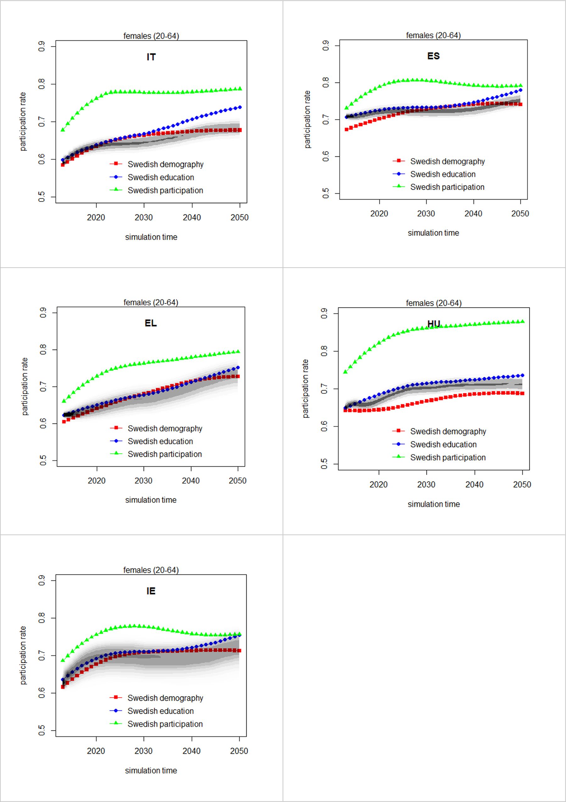
Figure 2 reports, for each country, the projected participation rates in the three baseline drivers scenarios: demographic evolution, educational attainments, and participation behaviour. The shaded areas in grey in the background represent uncertainty around the baseline projections, against which each scenario can be evaluated.10

Participation rates in the baseline drivers scenarios, female population aged 20–64 years. The shaded areas are the estimated densities of the baseline projections, computed over 1,000 replications with bootstrapped values of the coefficients.
In all countries, the gap in female participation with respect to Sweden is explained mostly by differences in the individual conditional behaviour, rather than in the composition of the population: ceteris paribus, conditional on individual characteristics, Swedish women are more active. This can be seen from the projections in the Swedish participation scenario, which are consistently and significantly higher than the baseline (5–10 ppt in Spain, Greece and Ireland; 10–15 ppt in Italy and Hungary). If women in Italy, Spain and Greece would have the same labour market behaviour of Swedish women, they would approach, by the end of the forecasting horizon, participation rates close to 80%, not far away from the near 90% value projected for Sweden (see Table 6).
Note that the result that behaviour matters more than individual characteristics in explaining the participation gap does not mean that the characteristics of the female population in the low-participation countries are similar to those of the Swedish population (they are not): what our analysis shows is that these differences do not matter much, as Swedish women participate more regardless of their attributes.
Indeed, endowing the low-participation countries with Swedish demography or Swedish education leads only to minor changes in participation rates. In particular, demography is actually helping Hungary and – up to around 2030 – Spain, in driving up participation rates with respect to Sweden, as can be seen by the fact that the projections for the Swedish demography scenario lie below the baseline. Differences in educational attainments play a role in explaining the participation gap with respect to Sweden, albeit relatively small (up to 2–3 ppt, 5 ppt in Italy), and concentrated in the second half of the simulation horizon, when the new hypothetical “Swedish like” cohorts will have replaced the old population.
The picture changes dramatically when focusing on the younger cohorts in childbearing years, where the participation gap with respect to Sweden is less pronounced (Table 7), except in Greece.
Participation rates and participation gaps with respect to Sweden, female population aged 20–44 years, baseline scenario
| Females (20–44 years old) | |||||
|---|---|---|---|---|---|
| Year | 2013 | 2020 | 2030 | 2040 | 2050 |
| Participation rates (%) | |||||
| Sweden | 84.2 | 84.6 | 86.1 | 85.1 | 85.6 |
| Spain | 76.8 | 77.5 | 73.8 | 74.5 | 76.5 |
| Hungary | 71.7 | 73.7 | 74.3 | 74.1 | 74.6 |
| Ireland | 68.1 | 74.4 | 69.3 | 68.9 | 73.6 |
| Greece | 66.2 | 64.1 | 63.3 | 62.7 | 62.1 |
| Italy | 64.7 | 70.8 | 71.2 | 71.1 | 72.1 |
| Participation gap w.r.t. Sweden (%) | |||||
| Spain | 9.6 | 10.8 | 15.8 | 14.9 | 13.2 |
| Hungary | 14.7 | 14.6 | 15.3 | 15.3 | 15.1 |
| Ireland | 18.3 | 13.9 | 20.3 | 20.5 | 16.1 |
| Greece | 20.2 | 24.2 | 26.3 | 26.7 | 27.6 |
| Italy | 21.7 | 17.5 | 18.4 | 18.3 | 17.6 |
The impact of the different drivers on the participation rates in this age group is shown in Figure 3. With the exception of Hungary, projections in the Swedish participation scenario for the 20–44 age group lie below the baseline, meaning that the conditional behaviour of younger women is not too different from their counterparts in Sweden, and if anything even more favourable to participation. Turning to differences in individual characteristics (the composition effect), Figure 3 shows that the lower educational attainments are responsible, as in the 20–64 years population, only for a small part of the participation gap (up to 2–3 ppt in all countries except Italy, where the participation rate would be five ppt higher, in the middle of the forecasting horizon, if women had the same educational attainments as in Sweden).11 Moreover, demography in this age group plays slightly in favour of low-participation countries, especially in the first part of the forecasting exercise (up to 2030). This is due to the fact that fertility rates are lower in these countries, hence the age distribution is more biased towards later ages (in the 20–44 years range), where participation is typically higher.
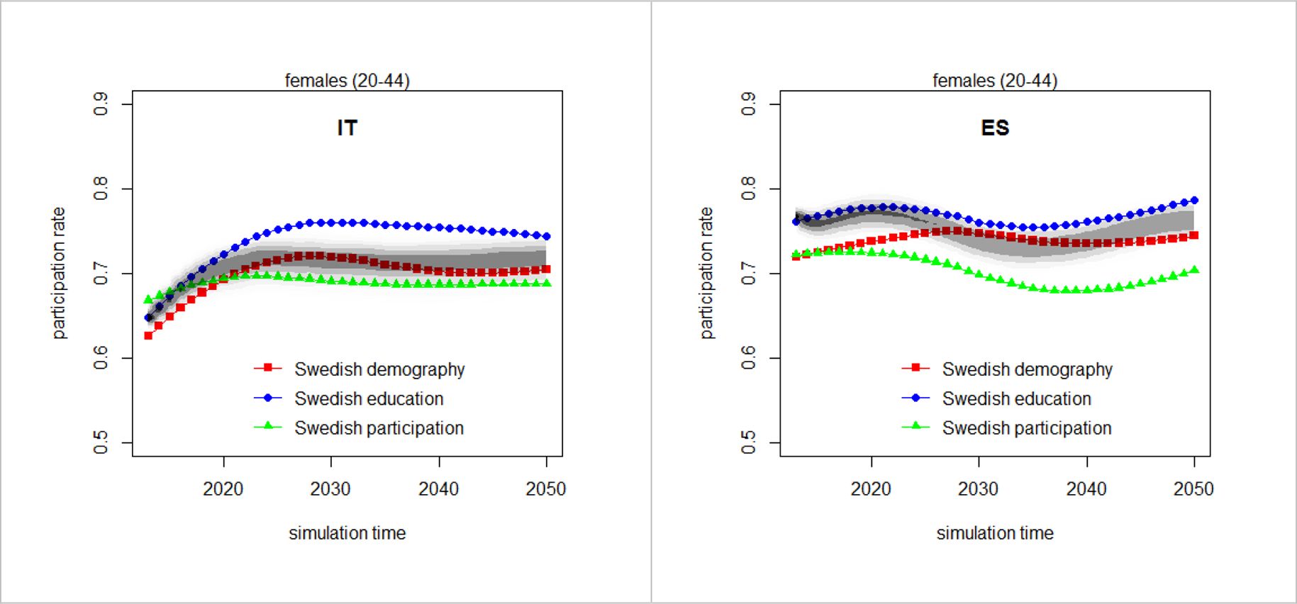

Participation rates in the baseline drivers scenarios, female population aged 20–44 years. The shaded areas are the estimated densities of the baseline projections, computed over 1,000 replications with bootstrapped values of the coefficients.
What other determinants are then responsible for the participation gap? In the participation equation, the only other individual characteristics considered are household composition, and participation and employment history (Table 1). However, the share of women in the 20–44 years old age range that are living in a union is higher in Sweden than in all other countries under analysis, so differences in household composition, if anything, play a role in attenuating the participation gap, rather than in explaining it. Part of the answer has to be found in the path persistent dynamics of participation itself: in Sweden it is easier to find employment; women are encouraged to participate in the labour market, even if only marginally, from an early age, and re-entry after maternity leave is facilitated. This has dynamic consequences as attachment to the labour market increases even at later ages.
To summarise our main findings so far, the low female participation rates in the countries under analysis can be explained mainly by an adverse behaviour of older women (even after controlling for differences in individual characteristics). Moreover, the behaviour of younger women is not detrimental to participation, their lower educational attainments are only partly responsible for the participation gap, and demography doesn’t help either in explaining it. The last source of the participation gap for women in childbearing years – in the model – is the role of family-friendly policies, and in particular the presence of public, affordable childcare, maternity leave, and part-time opportunities. As it turns out, inadequate family policies and part-time opportunities are important determinants of the low participation rates of younger women, thus completing our picture of the causes of the female participation gap: in short (and with some inevitable simplification) it is the adverse behaviour of older women, and insufficient policies and lack of opportunities for younger women.
The next section explores the impact of the family policy variables, together with policies aimed at increasing labour force participation at later ages by closing down opportunities for early retirement, and policies aimed at supporting aggregate demand, hence a faster recovery from the Great Recession.
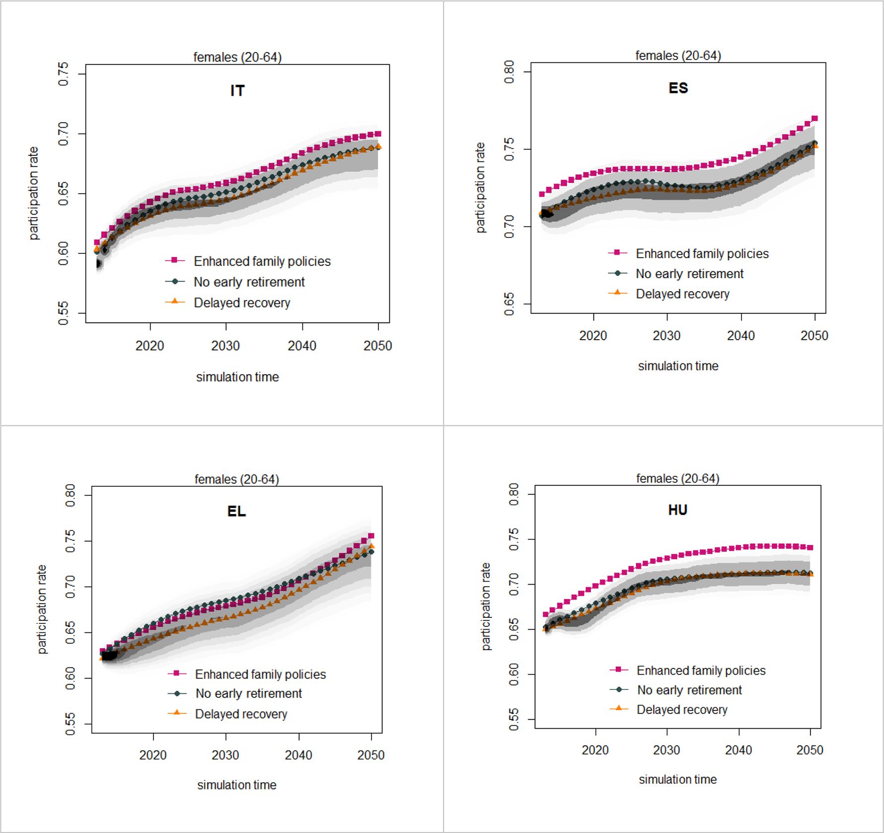
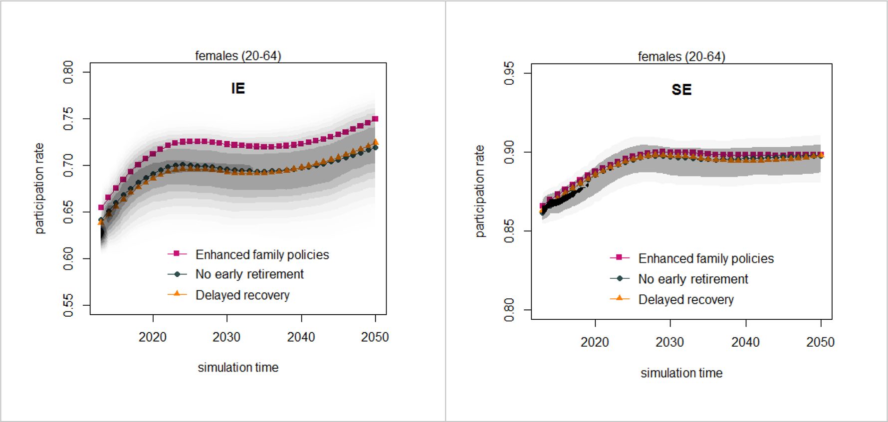
5. Results. The policy actions scenarios
Figure 4 is the analogue of Figure 2 for the policy actions scenarios. It shows, for each country, the projections for female participation rates in the age group 20–64 years, in the Enhanced family policies, No early retirement and Delayed recovery scenarios, against the background of the baseline. With the exception of Greece, where abolishing early retirements has an impact on aggregate participation rates of about two ppt in the mid 2020s, the only detectable effects at an aggregate level come from the Enhanced family policy scenario, with an increase in female participation rates that goes from 1 to 3 ppt. No further gains can be obtained, according to these projections, in Sweden. This is consistent with the findings of the previous section, as we pointed out that differences in conditional behaviour of women explain almost entirely, in the aggregate, the participation gap.

Participation rates in the policy actions scenarios, female population aged 20–64 years. The shaded areas are the estimated densities of the baseline projections, computed over 1,000 replications with bootstrapped values of the coefficients.
Moreover, the fact that these effects are small should be of no surprise, given that some of the policies have an impact on specific segments of the population only: in particular, childcare benefits and paid maternity leave are only relevant for mothers in childbearing years, for whom part-time opportunities also matter, while the abolition of early retirement options impacts only individuals who would otherwise retire before the new minimum retirement age. Accordingly, in the next sections we investigate the impact of the different scenarios in the most relevant subgroups of the population.
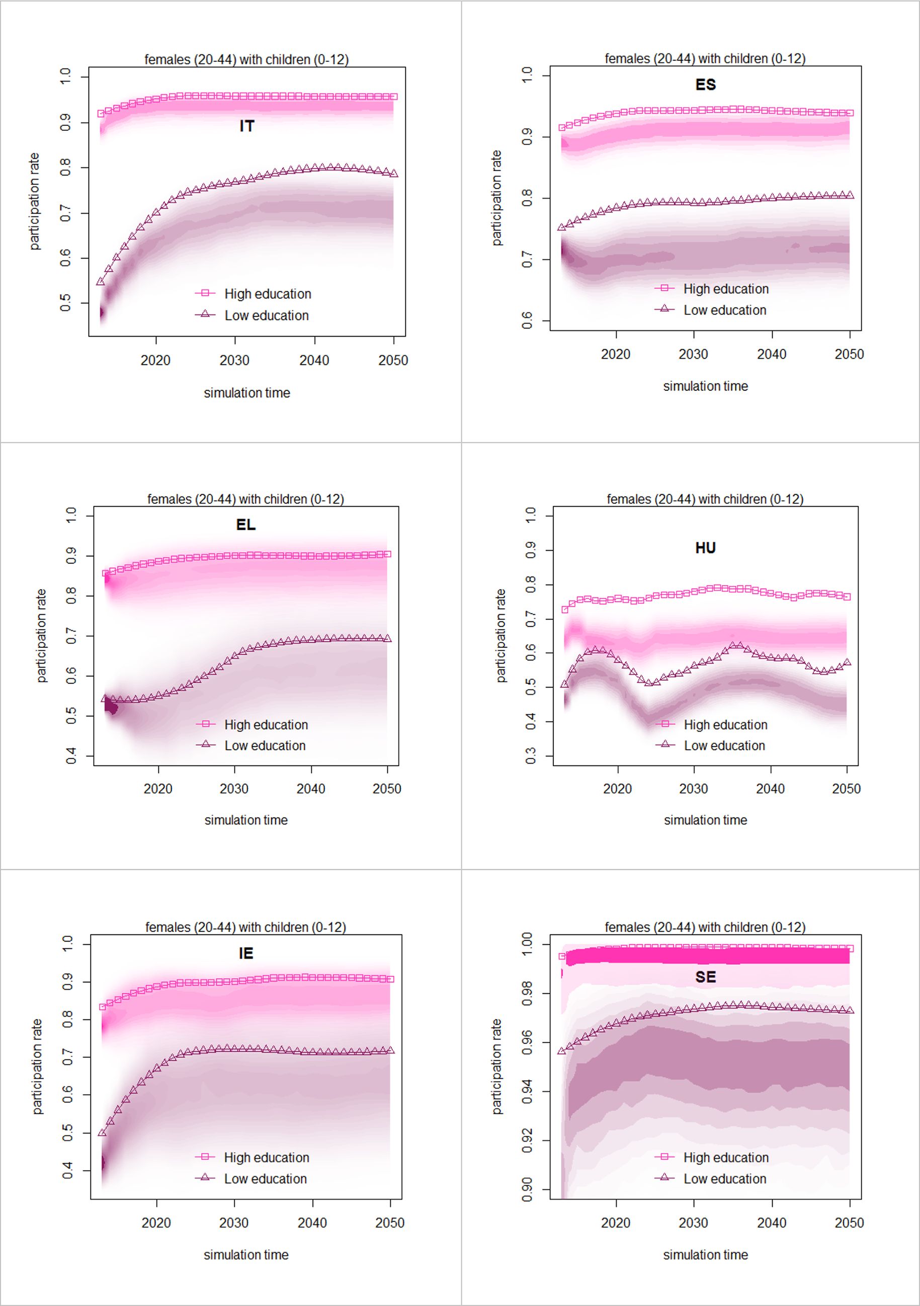
5.1. The enhanced family policies scenario
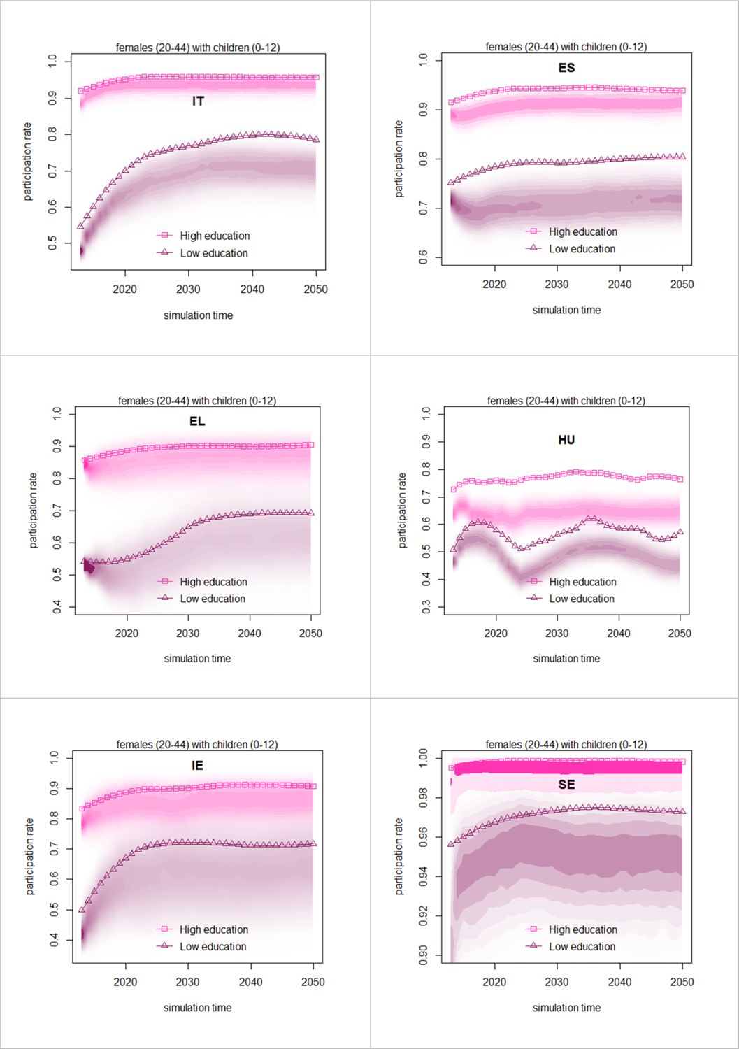
Figure 5 depicts projected participation rates in the Enhanced family policies scenario for mothers aged 20–44 years with children aged 0–12 years. For each country, we report participation rates separately for women with high and low education, against their respective baseline trends12. In all countries except Sweden, improving the family policies increases participation rates for women with low education by about 10 ppt, a remarkable amount. Even in Sweden, where participation rates are very high to start with, increasing childcare, on leave periods and part-time opportunities by 20% would increase the participation rate women with low education from about 95% to about 97%. Gains for highly educated women are more limited but still substantial, except in Hungary where both high and low educated women experience similar magnitudes of increase in participation.

Enhanced family policies scenario: public childcare benefits, duration of maternity leave and availability of part-time employment are jointly increased by 20%. Participation rates by educational attainments, female population aged 20–44 years not in education. The shaded areas are the estimated densities of the baseline projections, computed over 1,000 replications with bootstrapped values of the coefficients.
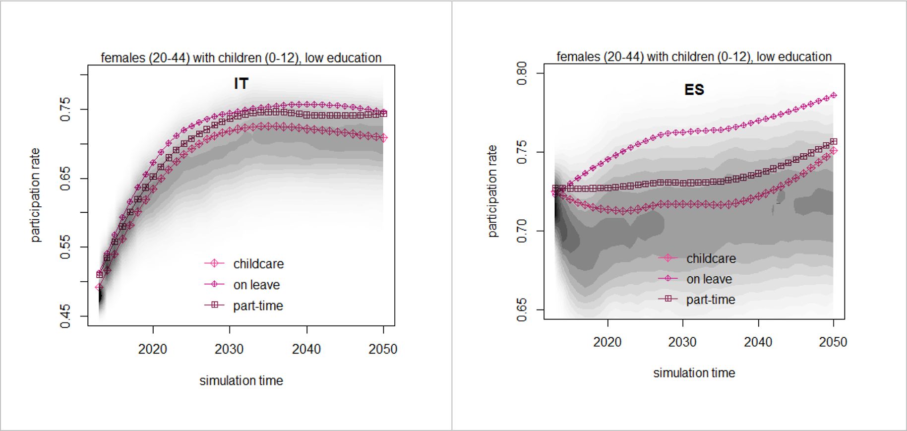
Finally, we explore the individual contributions of the different policies in the Enhanced family policy scenario: public childcare, maternity leave, and availability of part-time. For the sake of brevity, in presenting the results we focus on the most vulnerable group, in terms of participation: women (aged 20–44 years) with children (aged 0–12 years) and a low education. Figure 6 shows the effects of an increase of 20% in the values of each of these three scenario variables, separately. All variables have an effect, though it is their combination that drives participation rates up to the levels analysed above. In most countries, and in particular in Spain and Hungary, it is an increase in the duration of paid parental leave that is deemed to have the bigger effect (though the effects are generally so close that any difference is likely not to be robust to statistical testing). This is not surprising as maternity leave allows women to remain formally employed while taking care of their children.

Decomposition of the Enhanced family policies scenario: public childcare benefits, duration of maternity leave and availability of part-time employment are separately increased by 20%. Participation rates, female population aged 20–44 years with children aged 0–12 years and low education. The shaded areas are the estimated densities of the baseline projections, computed over 1,000 replications with bootstrapped values of the coefficients.
5.2. The no early retirement and the delayed recovery scenarios
Finally, we investigate the effects of the No early retirement and Delayed recovery scenarios in the sub-population of interest. Figure 7 reports the increase in the employment rate with respect to the baseline, due to a hypothetical minimum effective retirement age of 60 years old, both for males and females. The policy is evaluated on the population in the 50–59 age group. Despite the aggregate effects of this policy being negligible (see Figure 4) due to the relatively small size of the group of affected individuals, the effects on this sub-population are substantial, with an increase in the employment rate that peaks at almost 6 ppt in Greece, about 4 ppt in Hungary and Italy, and 2 ppt in Spain. The effects of raising the minimum effective retirement age obviously decline over time, as the average retirement age is expected to increase even without this additional policy – hence, the number of people that are affected, and would otherwise consider retiring before the newly imposed minimum retirement age, diminishes.
No early retirement scenario: minimum effective retirement age is 60 years old. Employment rates, differential to baseline, population aged 50–59 years.
As for what concerns the sensitivity of our results to the assumptions about the path of recovery from the crisis, Figure 8 shows that slowing down the recovery by 10 years reduces employment rates by about 3 ppt in Ireland, Spain and Greece, while smaller effects are expected elsewhere. These are the countries where the unemployment rate increases the most, with respect to the pre-crisis levels).

Delayed recovery scenario: the effects of the Great Recession fade away at a slower pace; complete recovery is achieved 10 years later than in the baseline (so 2040 in Greece and 2030 in other countries). Employment rates, differential to baseline, population aged 20–64.
6. Conclusions
Against a baseline scenario plotting a general trend of increasing participation rates towards the very high Swedish levels, where however Sweden will not be joined by any other country in meeting the Europe 2020 target, we have presented alternative scenarios aimed at understanding the drivers of the baseline results, and the expected effects of policies aimed at increasing participation and employment.
We argue that the low female participation rates in Italy, Spain, Greece, Hungary and Ireland, with respect to Sweden, are due to (i) low participation of older women, (ii), inadequate family policies and limited opportunities for family-work conciliation for younger women. According to our model, education plays a limited role, as older women with high education also participate little, and younger women in childbearing years are constrained by factors other than their level of education. An increase in the minimum retirement age is effective in keeping more women close to retirement in the labour force: however, due to the small number of women affected, the aggregate effects are small. Finally, a prolonged state of labour market distress due to the consequences of the Great Recession would push countries further away from the Europe 2020 targets, though again a lack of aggregate demand is not a primary explanation for the low observed female participation rates, and their incomplete projected convergence to the Swedish benchmark.
In fact, in the so called ‘baseline drivers’ alternative scenarios, by endowing low participation countries with ‘Swedish features’, possibly involving extreme, highly hypothetical departures from the baseline parameters, we learn that the gap in female participation with respect to Sweden is explained mostly by differences in the individual conditional behaviour, rather than in the composition of the population by age and education. Interestingly, this result turns out to be driven by older cohorts, i.e. people aged 45 years or more in the initial population. The conditional behaviour of younger women is not too different from their counterparts in Sweden, and if anything it is even more favourable to participation. Putting it differently, this indicates that there is not much room for manoeuvre to increase participation through higher education, and little can be done about the effect of choices made far in the past by older cohorts of women regarding their participation in the labour market.
Indeed, population ageing is a powerful as well as ‘automatic’ driver of participation, given that older cohorts tend to participate less, notwithstanding policies aimed at raising retirement age and creating incentives to extend their permanence in the labour force. Whilst population ageing might well create important labour supply shortages in the future, differences in the demographic trends cannot explain the incomplete and inadequate expected convergence to Swedish participation rates. Indeed, as many low-participation countries in the past few decades have experienced a stronger demographic transition than Sweden, with dramatic shrinkage of their younger cohorts, demographic evolution will contribute positively to convergence, as the relatively larger older cohorts, characterised by low participation rates, will gradually exit working age.
With respect to education not being an important policy lever to increase participation – a somehow counterintuitive result – it should be noted that this is consistent with the literature, which finds a significant effect of education on participation, but does not identify education policies as a key area of intervention (Jaumotte, 2004; Thévenon, 2013). Education matters a lot in explaining current participation levels of the older cohorts, as older women with low education often never considered entering the labour force, and is still significant in explaining current participation levels of younger generations because of the lower returns women with low education can expect from their participation in the labour market, both in terms of a lower probability of finding a job and lower wages. At the same time, education is less relevant for explaining future participation changes because (i) younger women in low-participation countries have already closed most of their education gap, with respect to benchmark countries like Sweden, and (ii) the premium that education commands with respect to unemployment and pay for younger women has also shrunk, partly due to increasing work insecurity and labour market dualisation, with young women getting a disproportionate share of ‘bad’ jobs, irrespective of their education level (Berton et al., 2012).
The reason for persistently low participation of prime age women has therefore to be found in the economic and institutional environment in which they live: our model highlights that inadequate family policies and part-time opportunities are important determinants of the observed and projected low participation rates. This is consistent with the findings of the literature, which point to the importance of flexibility of working-time arrangements and support to families with young children (ILO-IMF-OECD-WBG, 2014) as key policy drivers of female participation rates.
Indeed, there is a whole set of family friendly policies that would be desirable but are not implemented to a sufficient degree, because of - but not solely due to - budgetary constraints imposed by austerity. In particular, in our “policy actions” alternative scenarios, we have discussed two sets of family-work conciliation policies: first, policies that would facilitate women to perform both family and labour market related tasks (part time work, maternity leave); second, those that would allow women to access services provided by professionals that could substitute them in several basic care tasks (public childcare, but also elderly care or subsidies to families in order for them to hire caregivers).
The first set of policies (part time jobs and parental leave) has the downside to detach women – at least partially – from the labour market, with the risk of not being able to revert in the future to full participation. Moreover, such policies require cooperation on the side of firms, which should accommodate (costly) part timers and on-leave mothers without penalizing their career. Incentives and support from the Governments are clearly needed to achieve this goal. For instance, most Swedish companies are flexible regarding parental duties, and employees still get 80 per cent of their pay when they have to stay home with sick children or dependents. Yet, this does not happen at the expense of productivity: Sweden ranks ninth in the Global Competitiveness Index 2015–2016 (Ireland is 24th Spain 33rd, Italy 43rd, Hungary 63rd and Greece 81st; see Schwab, 2015).
Our reference country, Sweden, is also a leading example for parental leave policies. In Sweden, parents are entitled to 480 days of paid parental leave when a child is born or adopted. For 390 days, parents are entitled to nearly 80 per cent of their normal pay, up to a ceiling; the remaining 90 days are paid at a flat rate; those who are not in employment are also entitled to paid parental leave. The measure is financed to a large extent by employers’ contributions and for the remaining part (about a quarter) by general taxation. Parental leave can be taken up until a child turns eight years old. The leave entitlement applies to each child (except in the case of multiple births), so parents can accumulate leave from several children. In this period, parents also have the legal right to reduce their normal working hours by up to 25%. The duration of parental leave in Sweden is very high by international standards and is perhaps Sweden’s most famous argument when it comes to being a child-friendly system. Generous parental leave is not sufficient by itself though, to ensure a family-work balance. Hungary provides even longer periods of parental leave: 156 weeks for either parent, with cash benefits totalling 70% of previous earnings, up to a ceiling, for insured parents in the first 104 weeks, and flat rate benefits for non-insured parents or for insured parents in the last 52 weeks (Addati et al., 2014). However, participation rates in Hungary are among the lowest in Europe, and are projected to grow only at a comparatively slow rate. The reason is that parental leave can backfire when gender equality is not firmly rooted in the workplace, as women might lose their attachment to the labour force, or end up being discriminated against. It is difficult to separate the directions of the causal link between attitudes and behaviours, a positive attitude towards female participation being both a prerequisite and a consequence of increased female participation. However, policies aimed at promoting gender equality favour both. In Sweden, for instance, each parent has two months of paid parental leave reserved exclusively for him or her. Should a father – or a mother for that matter – decide not to take them, they cannot be transferred to the partner. 85% of Swedish fathers take parental leave, and men in Sweden take nearly a quarter of all parental leave. Those who don’t take the leave face questions from family, friends and colleagues. And in an effort to further improve these figures, the government provides a gender equality bonus, consisting of an extra daily payment if 270 days of the paid parental leave are divided evenly between the mother and the father.
The second set of policies (child care services and subsidies) has fewer downsides regarding the risk of detaching women from the labour market, but is more costly for the public budget and requires a strong political will to engage in long-term investments aimed at empowering women and sustaining families. In our reference country, Sweden, public childcare is guaranteed to all parents and it operates on a whole-day basis: most childcare facilities are open from 6.30 a.m. until 6.30 p.m. Pre-school is free for children aged between three and six years old for up to 15 hours per week. Aside from paid leave, the government provides an additional monthly child allowance until a child reaches the age of 16 years old, which covers the cost of additional childcare in pre-school years. Education for children aged six years old to university level is free of charge. The list of family friendly policies could proceed further. In 2010, for instance, the Swedish government introduced a new rule into its social insurance scheme to help single parents who fall ill and cannot look after their child. The rule allows another insured person (i.e. a person legally living and/or working in Sweden) who forgoes paid work to receive temporary parental benefits to look after the child. Low income parents may be entitled to a housing allowance. Parents pushing infants and toddlers in prams and pushchairs can ride for free on public buses. All in all, the government is an active player in structuring the whole society around the needs of young families.
In conclusion, our study points to the prominent role of family policies: what is needed is not a change of behaviour on the part of women (which has already happened), nor a rebalancing of the demographic structure (which will inevitably happen), but a change of mentality on the side of institutions and firms, which could prompt much needed further changes in the role of women in our societies at large.
As for what regards the directions for future research, at least two avenues seem promising, given the results achieved by the present study. First, the microsimulation analysis could be extended to all European member states, with the purpose of providing a scoreboard of indicators and scenarios of projected participation rates, extending the rather limited analysis by sub-groups of the population in existing studies. Second, the model could be extended to include income dynamics, allowing for more distributional analysis, for instance with respect to inequality and poverty. Finally, a more promising, as well as challenging one, would be to design a structural labour supply model based on a tax-benefit model (EUROMOD), by country.
Footnotes
1.
The latter is used mostly for policy parameters, as within country variation in policy settings over time is quite limited in the short run. In doing so we obtain average policy effects computed over 6 countries whose heterogeneity provides the needed variability.
2.
The microsimulation model is described in details in Richardson et al., (2018) as well as – more briefly – in the Appendix to the present work. It is developed using the JAS-mine simulation platform (Richiardi and Richardson, 2017) available open source from the JAS-mine website (see http://www.jas-mine.net/demo/labour-force-participation).
3.
The model simulates the following state variables of the individuals: age, gender, region, educational attainment, labour market status (student, employed, unemployed, retired or other inactive), cohabitation status (for females only), and number and age of children (for females only). It is estimated for the 6 mentioned countries based on the 2005–2011 waves of the EU-SILC longitudinal panel. The initial population is an extraction from the 2011 wave of the EU-SILC cross-sectional data.
4.
The relationship between participation and employment rates is given by the following equation:
EMPL_RATE = #EMPLOYED / POP = #ACTIVE (1-u) / POP = PART_RATE (1-u)
where EMPL_RATE is the employment rate, PART_RATE is the participation rate, #EMPLOYED is the number of employed individuals, #ACTIVE is the number of active individuals participating in the labour market, POP is the working age population and u is the aggregate unemployment rate, a scenario parameter in the model. Hence, given a value of u, a higher participation rate translates one-to-one into a higher employment rate.
5.
The estimated coefficients are also referred to in the econometric literature as returns to the covariates. The rationale for using the term ‘returns’ is better understood when thinking of monetary variables like income (which are absent in the microsimulation model), where for instance high education commands a positive return (a premium).
6.
The values of the estimated coefficients are reported in Appendix A of our companion paper.
7.
As already discussed, the decision to focus on participation stems from the centrality of participation in the model: employment, the other outcome of interest, is computed on the basis of participation, conditional on individual characteristics but aligned to match externally provided aggregate projections (variation of these scenario parameters is explored in the Delayed recovery scenario, see below).
8.
The Demographic module ages all individuals in the population and then passively aligns the population to Eurostat projections, by gender, age and simulation time. This means that at each simulated time the simulated population is partitioned by gender and age. The size of each resulting cell is then compared and aligned to the Eurostat projections. In this scenario we pretend that all countries are Sweden.
9.
Also Appendix B of our companion paper.
10.
Assessing the statistical significance of the differences with respect to the baseline would entail performing an assessment of the uncertainty of the projections in all the different scenarios, in addition to the one performed around the baseline. We leave this for future research. While being somewhat loose from a statistical perspective, the graphical analysis shown here gives a pretty good idea of the “economic significance” of the different results, and is a big improvement on the state of the art of simulation modelling (see our companion paper for a more in-depth discussion on this point).
11.
The effects of education are computed assuming a convergence to Swedish educational levels. These results can also be used to get a first order intuition about the effects of more plausible incentives to acquire further education. For instance, at the beginning of the simulation period, Italy – the country with the lowest educational attainments – has a share of women aged 20–44 years with low education of 27.8% (not considering students), compared to 6.5% in Sweden. Under the Swedish education scenario, the participation rate in Italy is 2.2 ppt higher than the baseline, in 2050. Using a linear interpolation, to achieve an increase in participation of 1 ppt in 2050 with respect to the baseline, a fairly limited objective, the share of women with low education in Italy should be pushed down to around 15%, an impressive achievement for education policies. Similar results hold for Spain. To put it differently, education policies are simply not a promising area of intervention to increase participation and hence move towards the Europe 2020 employment targets (though they might be important to achieve other policy objectives)
12.
Results for Hungary are subject to more oscillation due to sample variability in the original EU-SILC data.
References
-
1
Maternity and paternity at work. Law and practice across the worldGeneva: International Labour Office.
-
2
Explaining changes in female labor supply in a life-cycle modelAmerican Economic Review 98:1517–1552.https://doi.org/10.1257/aer.98.4.1517
-
3
The political economy of work security and flexibility: Italy in comparative perspectiveBristol: Policy Press.
-
4
Working Hours and Job Sharing in the EU and USA: Are Americans Crazy? Are Europeans Lazy?Oxford University Press.
-
5
New mothers’ labour force participation in Italy: the role of job characteristicsLabour 19:79–121.https://doi.org/10.1111/j.1467-9914.2005.00324.x
-
6
Women’s employment: joining explanations based on individual characteristics and on contextual factorsAmerican Journal of Economics and Sociology 70:756–783.https://doi.org/10.1111/j.1536-7150.2011.00790.x
-
7
Social Policies, Labour Markets and Motherhood: a Comparative Analysis of European CountriesCambridge MA: University Press.
- 8
-
9
European women: why do(n’t) they workApplied Economics 42:1499–1514.https://doi.org/10.1080/00036840701721547
-
10
Achieving stronger growth by promoting a more gender-balanced economyReport prepared for the G20 Labour and Employment Ministerial Meeting in.
-
11
Female labour force participation: past trends and main determinants in OECD countriesFemale labour force participation: past trends and main determinants in OECD countries, OECD Economics Department Working Papers No. 376.
-
12
Female labour force projections using Microsimulation for six EU countriesThe International Journal of Microsimulation, 3.
-
13
JAS-mine: a new platform for microsimulation and agent-based modellingInternational Journal of Microsimulation 10:106–134.
-
14
Returning to work after childbirth in France, Italy, and SpainEuropean Sociological Review 15:179–194.https://doi.org/10.1093/oxfordjournals.esr.a018259
- 15
-
16
Family policies in OECD countries: a comparative analysisPopulation and Development Review 37:57–87.https://doi.org/10.1111/j.1728-4457.2011.00390.x
- 17
Article and author information
Author details
Funding
The research was partly funded by a grant from Eurofound. Project title: “The gender employment gap: Challenges and solutions”, lot 3: “Anticipating the future trend of female labour market participation and its impact on economic growth”.
Acknowledgements
Not applicable.
Publication history
- Version of Record published: August 31, 2019 (version 1)
Copyright
© 2019, Richardson et al.
This article is distributed under the terms of the Creative Commons Attribution License, which permits unrestricted use and redistribution provided that the original author and source are credited.