What happened to the ‘Great American Jobs Machine’?
- Centre for Microsimulation and Policy Analysis, University of Essex, UK
- Institute for New Economic Thinking at the Oxford Martin School, UK
- Collegio Carlo Alberto, Italy
- University of Oxford, UK
- University of California-San Diego, USA
Figures

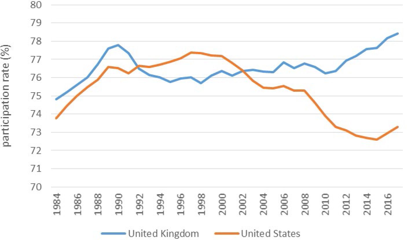
Labour force participation rates. Population aged 15–64.
Data source: OECD.

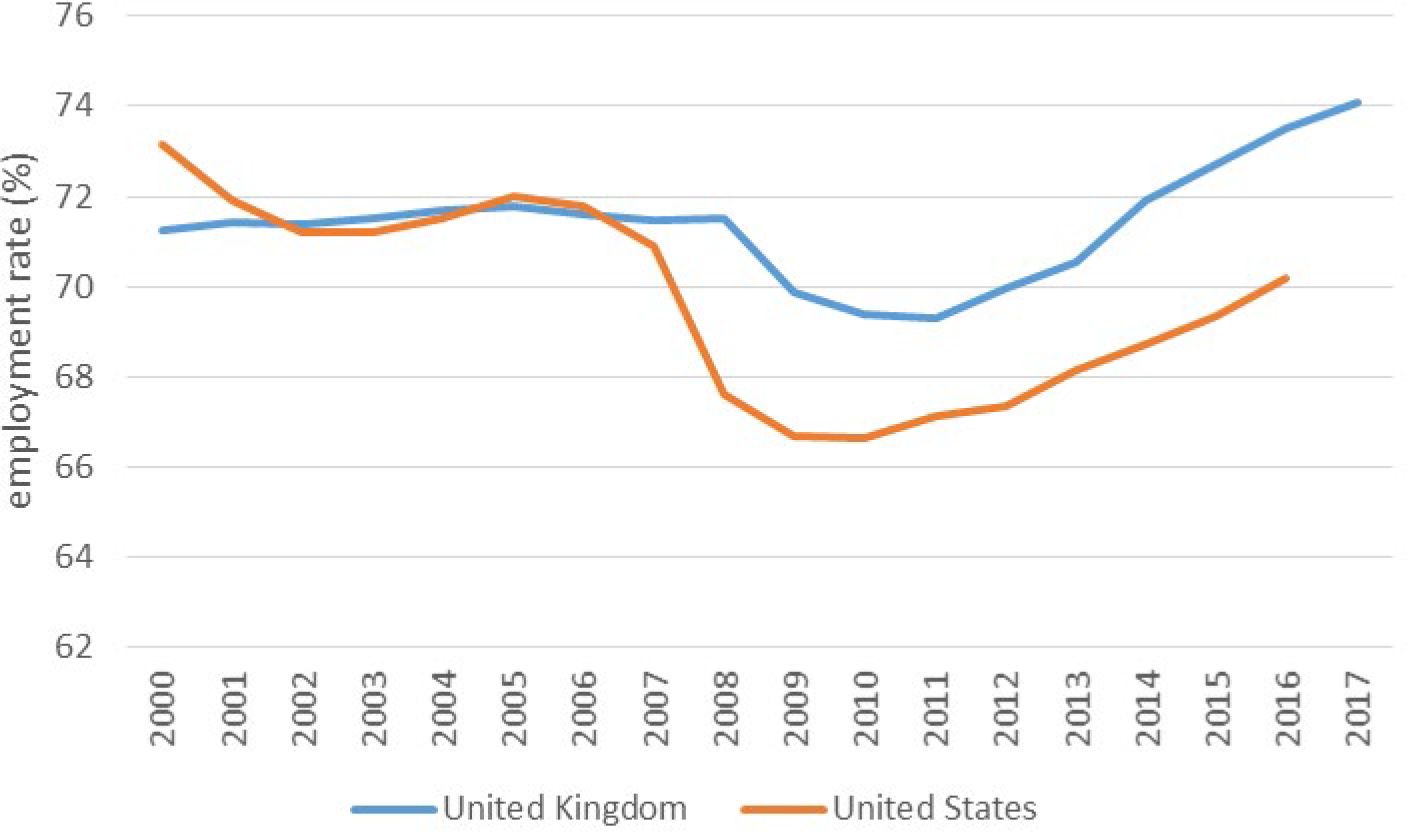
Employment rates. Population aged 15–64.
Data source: OECD.

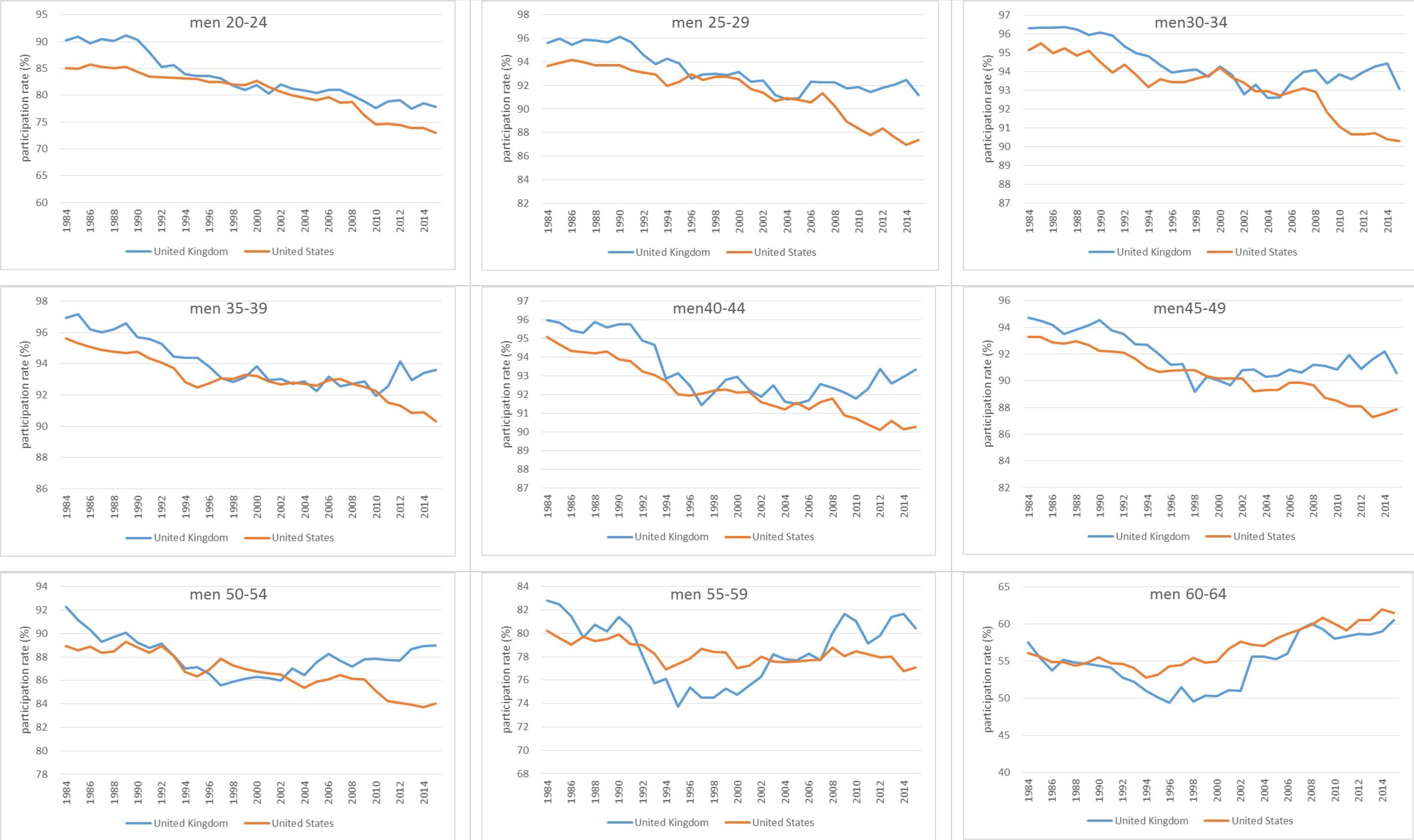
Male labour force participation rate by age group.
Data source: OECD.
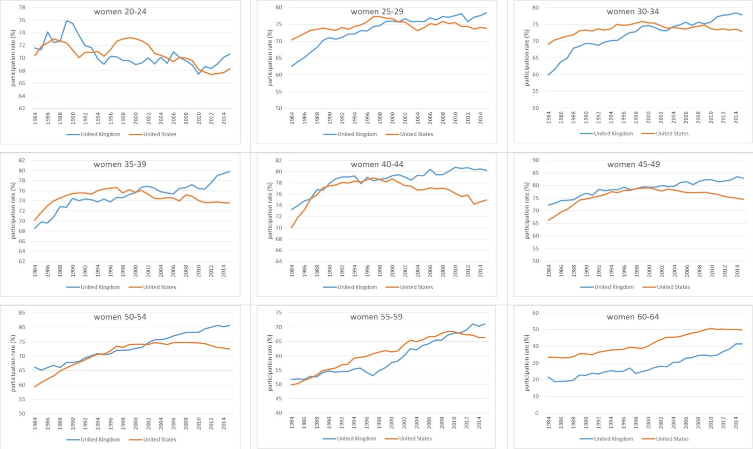
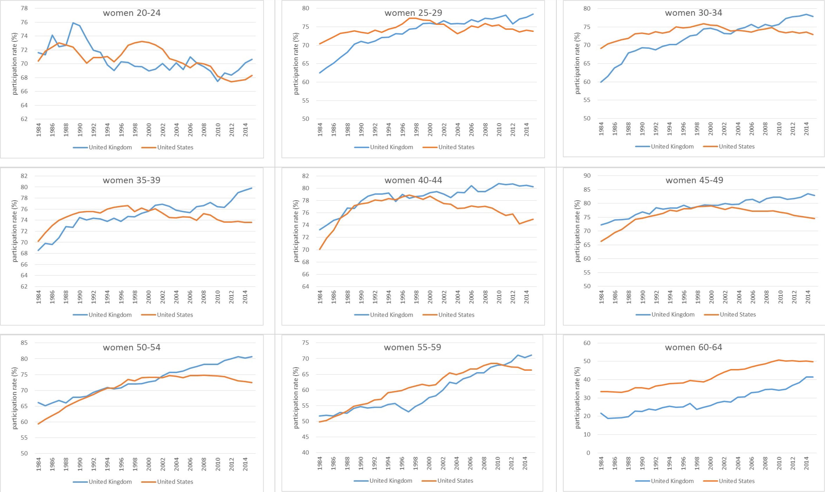
Female labour force participation rate by age group.
Data source: OECD.
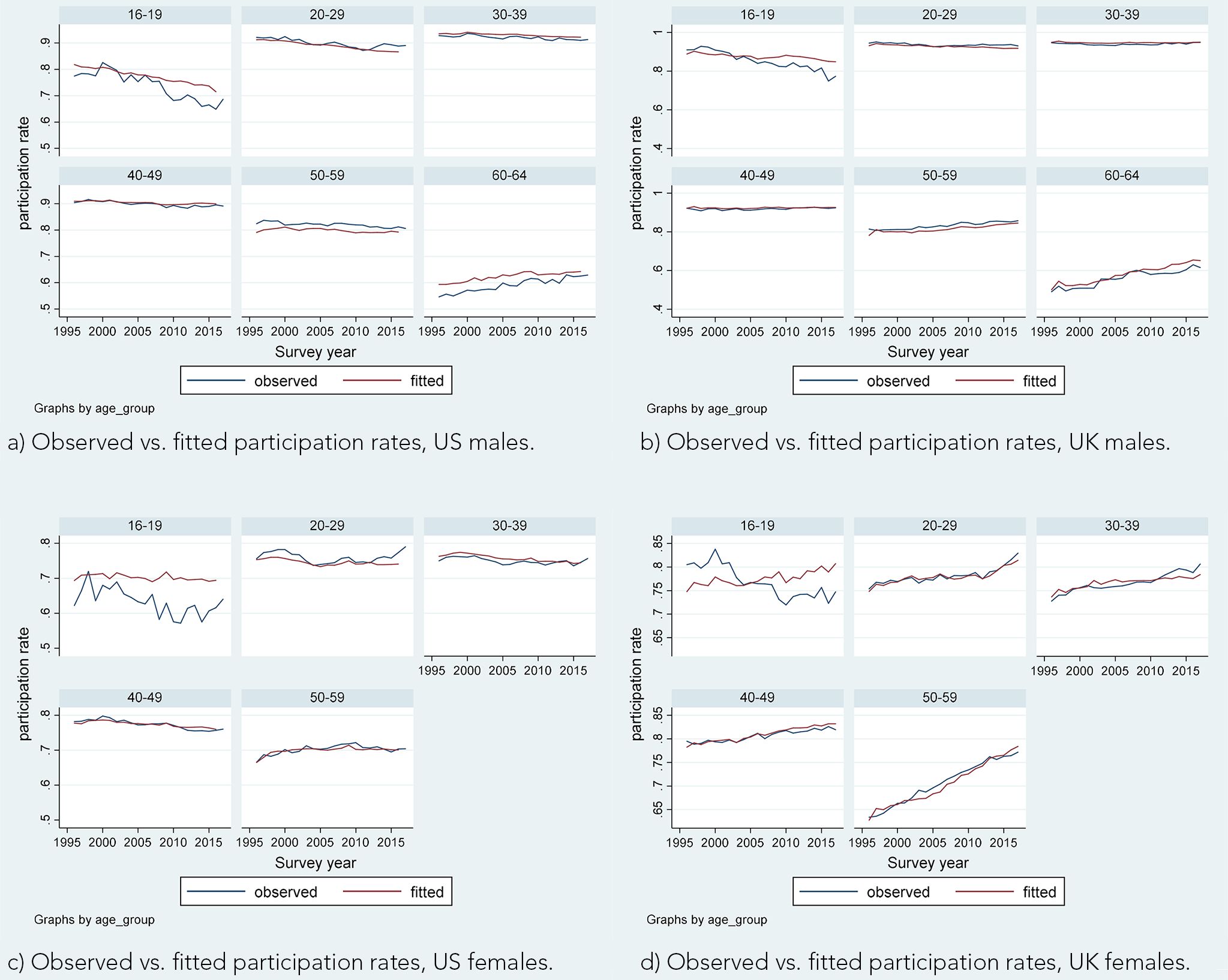
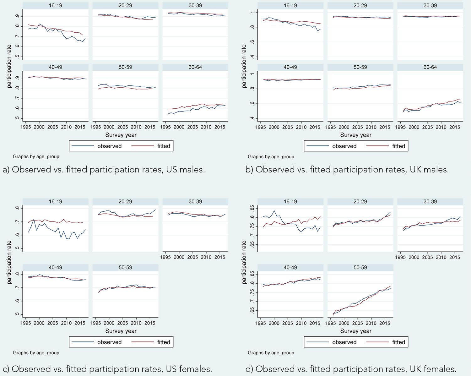
Observed vs. fitted participation rates, (a) US males, (b) UK males, (c) US females, (d) UK females. Coefficients as in Table 2.
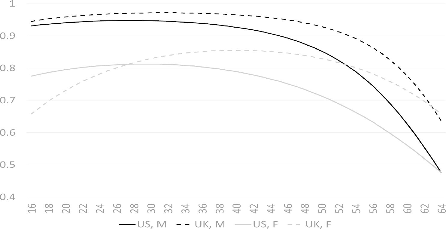

Estimated age effects: Participation probability at average values of other variables.

Estimated cohort effects: Participation probability at average values of other variables.
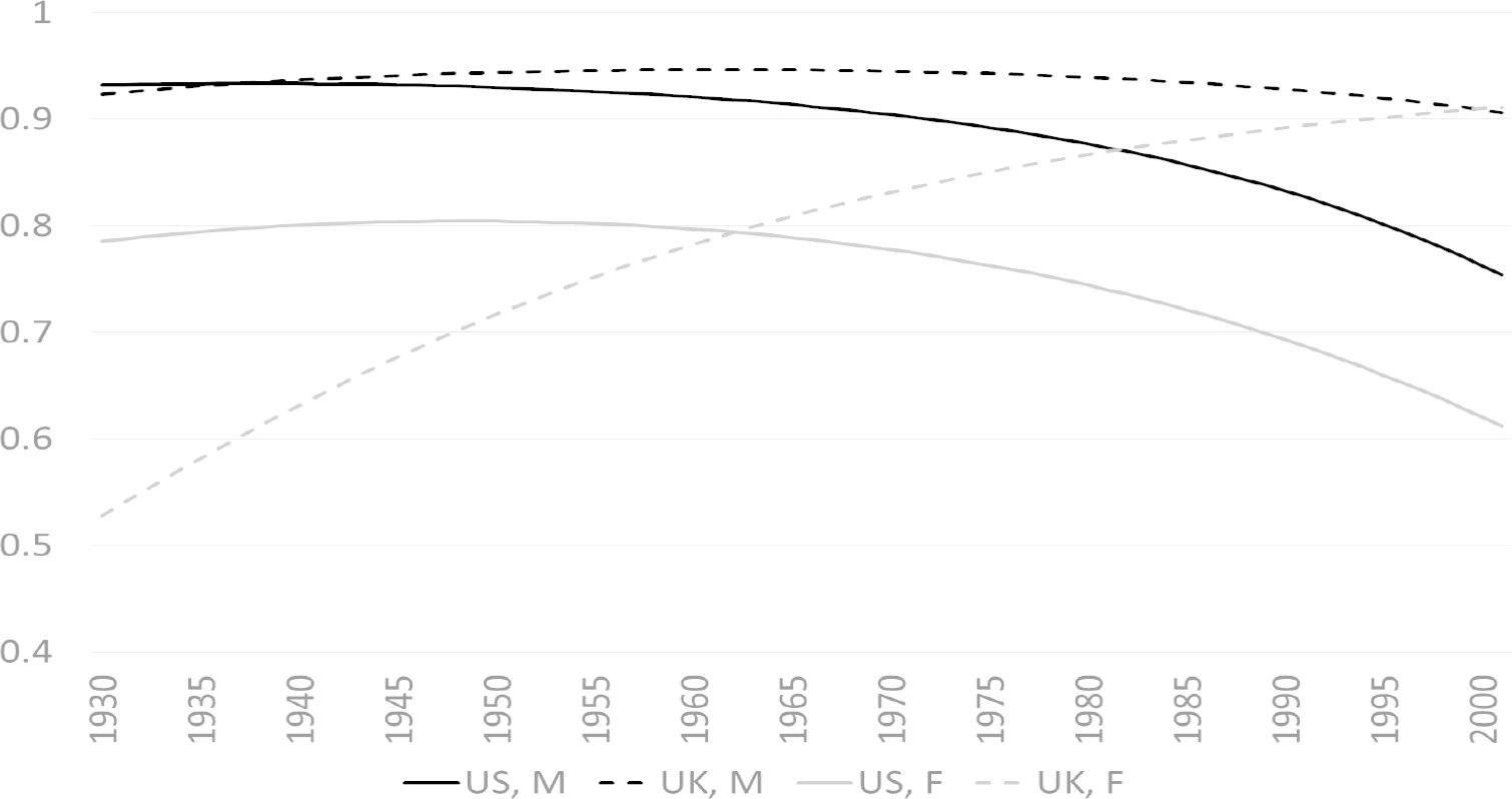

(a) Labour force participation rate, age 25–54, men, (b) Labour force participation rate, age 25–54, women The line for the United States is in bold.
Data source: OECD.

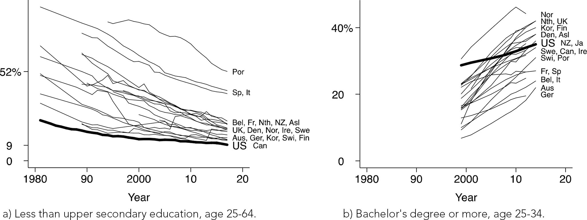
(a) Less than upper secondary education, age 25–64, (b) Bachelor’s degree or more, age 25–34. The line for the United States is in bold.
Data source: OECD.
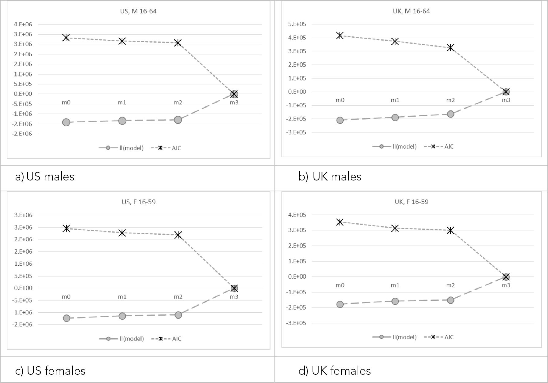

Goodness of fit, alternative models. Note: Each panel reports the log likelihood (ll) of the models and the Akaike Information Criterion (AIC), normalised by the values achieved by the best fit (m3). Higher is better for ll, while lower is better for AIC. Models as in table B1. (a) US males, (b) UK males, (c) US females, (d) UK females.
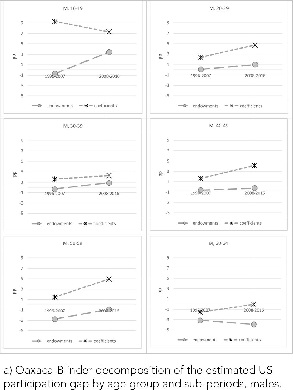

(a) Oaxaca-Blinder decomposition of the estimated US participation gap by age group and sub-periods, males.

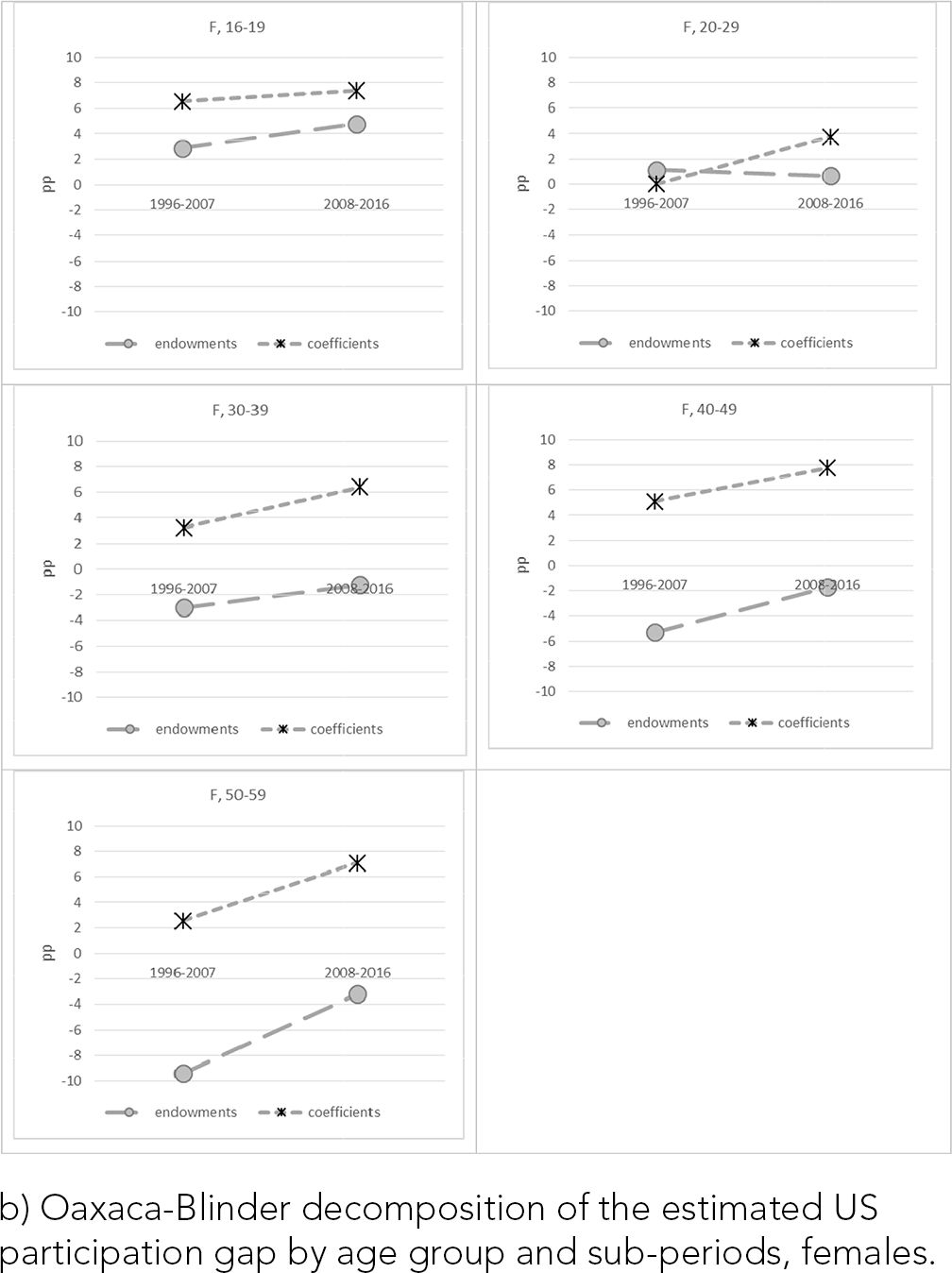
(b) Oaxaca-Blinder decomposition of the estimated US participation gap by age group and sub-periods, females.
Tables
Average values
| US | UK | ||||
|---|---|---|---|---|---|
| 1996 | 2017 | 1996 | 2017 | ||
| Active | 0.775 | 0.743 | 0.778 | 0.798 | |
| Student | 0.106 | 0.150 | 0.070 | 0.088 | |
| NEET (15-24) (a) | 0.232 | 0.220 | 0.241 | 0.175 | |
| Age | 37.0 | 38.5 | 38.1 | 40.1 | |
| Year of birth | 1959.0 | 1978.5 | 1957.9 | 1976.9 | |
| Race black | 0.099 | 0.123 | 0.015 | 0.030 | |
| Race other | 0.049 | 0.108 | 0.040 | 0.103 | |
| Hispanic | 0.152 | 0.204 | |||
| Foreign born | 0.150 | 0.192 | 0.078 | 0.177 | |
| Foreign national | 0.094 | 0.102 | 0.047 | 0.142 | |
| Education low | 0.202 | 0.156 | 0.359 | 0.164 | |
| Education medium | 0.581 | 0.545 | 0.442 | 0.447 | |
| Education high | 0.218 | 0.299 | 0.199 | 0.388 | |
| Household single alone | 0.272 | 0.312 | 0.260 | 0.283 | |
| Household single cohabiting | 0.020 | 0.043 | 0.054 | 0.121 | |
| Household married alone | 0.009 | 0.013 | 0.016 | 0.003 | |
| Household married cohabiting | 0.565 | 0.510 | 0.557 | 0.487 | |
| Household separated alone | 0.025 | 0.019 | 0.024 | 0.023 | |
| Household separated cohabiting | 0.002 | 0.003 | 0.004 | 0.003 | |
| Household divorced alone | 0.082 | 0.070 | 0.052 | 0.048 | |
| Household divorced cohabiting | 0.012 | 0.018 | 0.019 | 0.023 | |
| Household widowed alone | 0.012 | 0.011 | 0.013 | 0.009 | |
| Household widowed cohabiting | 0.001 | 0.002 | 0.001 | 0.001 | |
| Number of children | 0.953 | 0.950 | |||
| Household child under 2 (b) | 0.080 | 0.065 | 0.078 | 0.074 | |
| Household child 2–4 (c) | 0.090 | 0.084 | 0.114 | 0.116 | |
| Household child 5–9 (d) | 0.105 | 0.104 | 0.173 | 0.182 | |
| Household child 10–15 (e) | 0.105 | 0.111 | 0.210 | 0.206 | |
| Health bad | 0.092 | 0.097 | 0.152 | 0.139 | |
| Home owned | 0.664 | 0.645 | 0.729 | 0.646 | |
| Home owned outright | 0.154 | 0.199 | |||
| Home owned mortgage | 0.576 | 0.447 | |||
| Rural | 0.220 | 0.172 | |||
| Unemployment rate (regional or state level) | 0.061 | 0.048 | 0.084 | 0.045 | |
| GDP per capita (national currency) | 29,615 | 58,081 | (2016) | 15,526 | 30,850 |
| Minimum wage (% of GDP per capita) (f) | 0.154 | 0.147 | (2016) | 0.000 | 0.233 |
| Social expenditure family (% of GDP) (g) | 0.5 | 0.7 | (2016) | 2.2 | 3.8 |
| Social expenditure total (% of GDP) (h) | 14.8 | 19.3 | (2016) | 18.1 | 21.5 |
| Maternity total protected (weeks) (i) | 12 | 12 | (2016) | 40 | 70 |
| Maternity total paid (weeks) (j) | 0 | 0 | (2016) | 18 | 39 |
| Paternity total specific (weeks) (k) | 12 | 12 | (2016) | 0 | 20 |
| Paternity total specific paid (weeks) (l) | 0 | 0 | (2016) | 0 | 2 |
| AFDC/TANF/SNAP (m) | 29.3 | 21.2 | (2016) | ||
| SSI federal (n) | 16.4 | 13.4 | (2016) | ||
| EITC2max (o) | 124.0 | 102.0 | (2016) | ||
| EITC state (p) | 0.027 | 0.160 | (2016) | ||
-
a
Not in employment, education or training.
-
b
UK: presence of children below 2. US: youngest child below 2.
-
c
UK: presence of children aged between 2 and 4. US: youngest child aged between 2 and 4.
-
d
UK: presence of children aged between 5 and 9. US: youngest child aged between 5 and 9.
-
e
UK: presence of children aged between 10 and 15. US: youngest child aged between 10 and 15.
-
f
UK: national minimum wage. US: state minimum wage. Normalised by GDP per capita (000).
-
g
Social expenditures on family policies (% of GDP).
-
h
Social expenditures, total (% of GDP).
-
i
Maximum weeks of job-protected maternity, parental and home care leave available to mothers, regardless of income support.
-
j
Total weeks of paid maternity, parental and home care payments available to mothers.
-
k
Total weeks of leave reserved for exclusive use by the father.
-
l
Total weeks of paid leave reserved for exclusive use by the father.
-
m
Combined monthly maximum AFDC/TANF and Food Stamps benefits for a 4-person family. Normalised by GDP per capita and multiplied by 1,000.
-
n
EITC maximum credit for two dependents. Normalised by GDP per capita (000).
-
o
Monthly maximum federal SSI benefits for individuals living independently. Normalised by GDP per capita (000).
-
p
State EITC rate as percentage of Federal credit.
Logit estimates of the probability of being in the labour force
| (1) | (2) | (3) | (4) | |||||
|---|---|---|---|---|---|---|---|---|
| US | UK | US | UK | |||||
| Male | Male | Female | Female | |||||
| Variables | 16–64 | 16–64 | 16–59 | 16–59 | ||||
| Age | 0.123 | *** | 0.178 | *** | 0.076 | *** | 0.156 | *** |
| Age squared | −0.002 | *** | −0.003 | *** | −0.001 | *** | −0.002 | *** |
| Year of birth | 0.029 | *** | 0.047 | *** | 0.034 | *** | 0.056 | *** |
| Year of birth squared | 0.000 | *** | 0.000 | *** | 0.000 | *** | 0.000 | *** |
| Race black | −0.479 | *** | −0.315 | *** | 0.174 | *** | 0.231 | *** |
| Race other | −0.367 | *** | −0.447 | *** | −0.109 | *** | −0.712 | *** |
| Foreign born | 0.311 | *** | 0.222 | *** | 0.003 | −0.063 | *** | |
| Foreign national | 0.112 | *** | −0.082 | *** | −0.519 | *** | −0.043 | *** |
| Hispanic | 0.111 | *** | 0.105 | *** | ||||
| Education high | −31.25 | *** | −4.44 | −24.42 | *** | 10.35 | *** | |
| Education low | 3.050 | 5.772 | * | −13.140 | *** | 25.070 | *** | |
| Health bad | −8.532 | ** | −47.640 | *** | 29.210 | *** | 0.993 | |
| Year x health | 0.003 | * | 0.023 | *** | −0.015 | *** | −0.001 | |
| Year x education high | 0.016 | *** | 0.002 | 0.012 | *** | −0.005 | *** | |
| Year x education low | −0.002 | −0.003 | * | 0.006 | *** | −0.013 | *** | |
| Household single cohab | 0.735 | *** | 0.617 | *** | 0.191 | *** | 0.212 | *** |
| Household married alone | 0.639 | *** | 0.804 | *** | −0.050 | * | −0.167 | *** |
| Household married cohab | 0.899 | *** | 0.730 | *** | −0.384 | *** | −0.141 | *** |
| Household separated alone | 0.443 | *** | 0.361 | *** | 0.200 | *** | 0.037 | * |
| Household separated cohab | 0.548 | *** | 1.030 | *** | 0.063 | 0.399 | *** | |
| Household divorced alone | 0.486 | *** | 0.307 | *** | 0.315 | *** | 0.206 | *** |
| Household divorced cohab | 0.793 | *** | 0.689 | *** | 0.197 | *** | 0.300 | *** |
| Household widowed alone | 0.133 | *** | 0.238 | *** | −0.431 | *** | −0.084 | *** |
| Household widowed cohab | 0.351 | *** | 0.544 | *** | −0.248 | *** | 0.059 | |
| Household child under 2 | 0.041 | −0.114 | *** | −0.967 | *** | −1.479 | *** | |
| Household child 2–4 | 0.013 | −0.205 | *** | −0.645 | *** | −1.283 | *** | |
| Household child 5–9 | 0.067 | *** | −0.225 | *** | −0.285 | *** | −0.759 | *** |
| Household child 10–15 | 0.169 | *** | −0.145 | *** | 0.071 | *** | −0.429 | *** |
| Number of children | 0.139 | *** | −0.094 | *** | ||||
| Home owned | 0.068 | *** | 0.182 | *** | ||||
| Unemployment rate | −1.215 | *** | −0.023 | 0.615 | ** | −0.038 | ||
| Post-crisis | 0.116 | *** | 0.089 | ** | 0.083 | *** | 0.043 | |
| Minimum wage | −0.546 | −0.243 | * | 0.910 | *** | −0.010 | ||
| Social expenditure family | −0.104 | ** | −0.031 | 0.091 | ** | 0.005 | ||
| Social expenditure total | −0.008 | −0.010 | −0.021 | ** | −0.008 | |||
| AFDC/TANF/SNAP | −0.014 | *** | −0.018 | *** | ||||
| SSI federal | 0.003 | 0.022 | ||||||
| EITC2max | 0.000 | 0.000 | ||||||
| EITC state | −0.022 | 0.019 | ||||||
| Rural | −0.137 | *** | 0.007 | |||||
| Home owned outright | 0.240 | *** | 0.320 | *** | ||||
| Home owned mortgage | 1.232 | *** | 1.056 | *** | ||||
| Maternity total protected | −0.007 | *** | −0.008 | *** | ||||
| Maternity total paid | 0.006 | *** | 0.000 | |||||
| Paternity total specific | 0.007 | * | 0.007 | *** | ||||
| Constant | 1.127 | *** | −0.792 | 0.461 | ** | −3.431 | *** | |
| Observations | 1,063,351 | 718,417 | 1053301 | 704,235 | ||||
| chi2 | 97,216 | 120,525 | 79,867 | 120,176 | ||||
| P | 0.000 | 0.000 | 0.000 | 0.000 | ||||
| r2_p | 0.239 | 0.364 | 0.118 | 0.246 |
-
Notes: Robust standard errors in parentheses *** p<0.01, ** p<0.05, * p<0.1.
-
Students excluded. The baseline is a medium education white individual, single and not cohabiting, living in urban California (US) or central London (UK), and renting. Cohort is measured subtracting 1,900 from year of birth. State (US) and NUTS1 (UK) regional dummies included.
Effects of education and health over time
| Males | Females | ||||||||
|---|---|---|---|---|---|---|---|---|---|
| US | UK | US | UK | ||||||
| Case | Reference category | 1996 | 2017 | 1996 | 2017 | 1996 | 2017 | 1996 | 2017 |
| Education High | Education Medium | 0.29 | 0.62 | 0.04 | 0.08 | 0.33 | 0.59 | 0.57 | 0.47 |
| Education Low | Education Medium | −0.58 | −0.62 | −0.40 | −0.46 | −0.80 | −0.67 | −0.48 | −0.75 |
| Health Bad | Health Good | −2.16 | −2.10 | −2.73 | −2.26 | −1.33 | −1.65 | −1.90 | −1.93 |
-
Notes: The table reports the contribution to the logit score from Table 2. The non-linearity of the logit function means that the same increase in the logit score has a different impact on the estimated probability depending on the starting value of the score.
Alternative specifications
| Model name | Treatment of period effect | Linear age and cohort effects identifiable | Policy effects identifiable |
|---|---|---|---|
| m0 | No period effects | Yes | No |
| m1 | Period effects captured by macroeconomic variables | Yes | Yes |
| m2 | Time dummies | No | only policy differentials in the US |
| m3 | Time*region dummies | No | No |
Oaxaca-Blinder decomposition of the estimated US participation gap, males
| Males, 16–64 | 1996–2007 | 2008–2017 | ||
|---|---|---|---|---|
| UK mean | 87.2% | 87.8% | ||
| US mean | 87.1% | 84.7% | ||
| difference UK-US (pp) | 0.14 | 3.12 | ||
| of which: | ||||
| endowments (pp) | −1.75 | −0.04 | ||
| coefficients (pp) | 1.83 | 3.86 | ||
| interaction (pp) | 0.06 | −0.70 | ||
| endowments | coefficients | Endowments | Coefficients | |
| Overall (pp) | −1.75 | 1.83 | −0.04 | 3.86 |
| Contribution of each covariate (pp): | ||||
| APC | −0.77 | −1.04 | −0.01 | −0.25 |
| Race black | 0.78 | 0.46 | −0.05 | 0.44 |
| Race other | 0.03 | −0.06 | 0.00 | −0.08 |
| Foreign born | −0.34 | 0.08 | 0.02 | 0.19 |
| Foreign national | −0.08 | −0.23 | −0.01 | −0.26 |
| Education high | −0.12 | −0.63 | −0.04 | −1.34 |
| Education low | −1.50 | 0.27 | 0.07 | 0.16 |
| Household single cohab | 0.61 | 0.01 | −0.06 | 0.07 |
| Household married alone | −0.14 | 0.05 | 0.01 | 0.06 |
| Household married cohab | −0.29 | −1.08 | 0.03 | 0.69 |
| Household separated alone | −0.00 | −0.02 | −0.00 | 0.09 |
| Household separated cohab | 0.02 | 0.01 | −0.00 | 0.03 |
| Household divorced alone | −0.27 | −0.13 | 0.01 | 0.11 |
| Household divorced cohab | 0.11 | 0.00 | −0.00 | 0.08 |
| Household widowed alone | 0.00 | 0.00 | 0.00 | 0.02 |
| Household widowed cohab | 0.00 | 0.00 | −0.00 | 0.00 |
| Household child under 2 | −0.00 | −0.27 | −0.01 | −0.25 |
| Household child 2–4 | −0.01 | −0.36 | −0.00 | −0.28 |
| Household child 5–9 | −0.00 | −0.35 | −0.00 | −0.38 |
| Household child 10–15 | 0.07 | −0.28 | −0.00 | −0.29 |
| Home owned | 0.16 | 5.41 | −0.00 | 5.07 |
| Unemployment rate difference | −0.02 | −0.00 | 0.00 | −0.00 |
-
Note: Cells with a positive (negative) contribution to the US participation gap of more (less) than one pp are highlighted in red (green).
Oaxaca-Blinder decomposition of the estimated US participation gap, females
| Females, 16–60 | 1996–2007 | 2008–2017 | ||
|---|---|---|---|---|
| UK mean | 75.1% | 78.6% | ||
| US mean | 74.9% | 74.0% | ||
| difference UK-US (pp) | 0.17 | 4.54 | ||
| of which: | ||||
| endowments (pp) | −4.05 | −1.17 | ||
| coefficients (pp) | 3.26 | 6.61 | ||
| interaction (pp) | 0.95 | −0.91 | ||
| endowments | coefficients | endowments | Coefficients | |
| Overall (pp) | −4.05 | 3.26 | −1.17 | 6.61 |
| Contribution of each covariate (pp): | ||||
| APC | −0.14 | −2.55 | 0.54 | 1.14 |
| Race black | −0.15 | 0.35 | −0.11 | 0.34 |
| Race other | 0.01 | −0.36 | −0.02 | −0.69 |
| Foreign born | −0.01 | −0.02 | −0.05 | 0.08 |
| Foreign national | 0.13 | 0.36 | −0.50 | 0.64 |
| Education high | −0.23 | 0.31 | 1.09 | −0.32 |
| Education low | −4.32 | 0.27 | −2.47 | −0.03 |
| Household single cohab | 0.30 | 0.06 | 0.56 | 0.10 |
| Household married alone | 0.02 | 0.02 | 0.01 | 0.00 |
| Household married cohab | 0.29 | 2.54 | 0.67 | 2.39 |
| Household separated alone | 0.01 | −0.01 | 0.01 | 0.03 |
| Household separated cohab | 0.00 | 0.01 | −0.00 | 0.02 |
| Household divorced alone | −0.25 | −0.11 | −0.15 | 0.12 |
| Household divorced cohab | 0.05 | 0.05 | 0.02 | 0.08 |
| Household widowed alone | 0.03 | 0.07 | 0.13 | 0.13 |
| Household widowed cohab | −0.00 | 0.01 | 0.01 | 0.02 |
| Household child under 2 | −0.02 | −0.95 | −0.51 | −0.87 |
| Household child 2–4 | 0.01 | −1.04 | −0.28 | −1.08 |
| Household child 5–9 | 0.02 | −0.76 | −0.03 | −0.69 |
| Household child 10–15 | −0.00 | −0.51 | −0.00 | −0.48 |
| Home owned | 0.23 | 5.51 | −0.06 | 5.68 |
| Unemployment rate difference | −0.04 | 0.00 | −0.01 | −0.00 |
-
Note: Cells with a positive (negative) contribution to the US participation gap of more (less) than one pp are highlighted in red (green).
Trends in educational attainment by gender (sample frequencies)
| Male | Female | |||||||
|---|---|---|---|---|---|---|---|---|
| US | UK | US | UK | |||||
| 1996 | 2017 | 1996 | 2017 | 1996 | 2017 | 1996 | 2017 | |
| Education Low | 0.210 | 0.167 | 0.320 | 0.182 | 0.194 | 0.145 | 0.399 | 0.146 |
| Education High | 0.229 | 0.279 | 0.210 | 0.366 | 0.206 | 0.319 | 0.189 | 0.411 |
Oaxaca-Blinder decomposition of the estimated US participation gap by age group and sub-periods, males
| Gender | Male | Male | Male | |||
|---|---|---|---|---|---|---|
| age group | 16–19 | 20–29 | 30–39 | |||
| Period | 1996–2007 | 2008–2016 | 1996–2007 | 2008–2016 | 1996–2007 | 2008–2016 |
| overall (pp) | 10.6 | 12.9 | 3.0 | 4.7 | 1.3 | 2.7 |
| endowments | −0.7 | 3.5 | 0.1 | 1.0 | −0.3 | 0.9 |
| Coefficients | 9.3 | 7.3 | 2.4 | 4.7 | 1.6 | 2.3 |
| Interaction | 2.1 | 2.1 | 0.5 | −1.1 | 0.0 | −0.5 |
| age group | 40–49 | 50–59 | 60–64 | |||
| Period | 1996–2007 | 2008–2016 | 1996–2007 | 2008–2016 | 1996–2007 | 2008–2016 |
| overall (pp) | 1.0 | 3.2 | –0.7 | 3.5 | –4.1 | –2.1 |
| endowments | −0.6 | −0.2 | −2.7 | −0.9 | −3.1 | −3.9 |
| Coefficients | 1.6 | 4.2 | 1.5 | 4.9 | −1.6 | 0.0 |
| Interaction | 0.0 | −0.8 | 0.6 | −0.5 | 0.6 | 1.9 |
Oaxaca-Blinder decomposition of the estimated US participation gap by age group and sub-periods, females
| Gender | Female | Female | Female | |||
|---|---|---|---|---|---|---|
| age group | 16–19 | 20–29 | 30–39 | |||
| Period | 1996–2007 | 2008–2016 | 1996–2007 | 2008–2016 | 1996–2007 | 2008–2016 |
| overall (pp) | 13.3 | 13.9 | 1.1 | 3.4 | –0.1 | 3.8 |
| endowments | 2.9 | 4.8 | 1.1 | 0.7 | −3.0 | −1.2 |
| Coefficients | 6.6 | 7.4 | 0.0 | 3.8 | 3.2 | 6.4 |
| Interaction | 3.9 | 1.7 | −0.1 | −1.0 | −0.3 | −1.4 |
| age group | 40–49 | 50–59 | ||||
| Period | 1996–2007 | 2008–2016 | 1996–2007 | 2008–2016 | ||
| overall (pp) | 1.4 | 5.5 | –2.5 | 4.2 | ||
| endowments | −5.3 | −1.7 | −9.4 | −3.2 | ||
| Coefficients | 5.1 | 7.8 | 2.5 | 7.1 | ||
| Interaction | 1.7 | −0.6 | 4.4 | 0.3 |
Logit estimates of the probability of being in the labour force, common specification, males. Students excluded
| (1) | (2) | (3) | (4) | |||||
|---|---|---|---|---|---|---|---|---|
| US | UK | US | UK | |||||
| M 16–64 | M 16–64 | M 16–64 | M 16–64 | |||||
| VARIABLES | 1996–2007 | 1996–2007 | 2008–2017 | 2008–2017 | ||||
| Age | 0.094 | *** | 0.066 | *** | 0.123 | *** | 0.154 | *** |
| Age squared | −0.002 | *** | −0.002 | *** | −0.002 | *** | −0.003 | *** |
| Year of birth | 0.038 | *** | 0.087 | *** | 0.007 | 0.022 | ** | |
| Year of birth squared | 0.000 | *** | −0.001 | *** | 0.000 | 0.000 | *** | |
| Race black | −0.583 | *** | −0.072 | −0.480 | *** | −0.058 | ||
| Race other | −0.492 | *** | −0.619 | *** | −0.376 | *** | −0.489 | *** |
| Foreign born | 0.347 | *** | 0.408 | *** | 0.442 | *** | 0.556 | *** |
| Foreign national | 0.189 | *** | −0.099 | *** | 0.352 | *** | 0.067 | ** |
| Education high | −13.91 | 6.15 | −34.72 | *** | 22.41 | * | ||
| Education low | −25.92 | *** | 13.19 | ** | −2.11 | 35.67 | *** | |
| Year x education high | 0.007 | * | −0.003 | 0.018 | *** | −0.011 | * | |
| Year x education low | 0.013 | *** | −0.007 | ** | 0.001 | −0.018 | *** | |
| Household single cohab | 0.764 | *** | 0.817 | *** | 0.758 | *** | 0.934 | *** |
| Household married alone | 0.766 | *** | 1.150 | *** | 0.772 | *** | 1.253 | *** |
| Household married cohab | 1.115 | *** | 0.884 | *** | 0.941 | *** | 1.085 | *** |
| Household separated alone | 0.529 | *** | 0.387 | *** | 0.263 | *** | 0.758 | *** |
| Household separated cohab | 0.670 | *** | 1.358 | *** | 0.454 | *** | 1.513 | *** |
| Household divorced alone | 0.512 | *** | 0.310 | *** | 0.387 | *** | 0.547 | *** |
| Household divorced cohab | 0.953 | *** | 0.965 | *** | 0.694 | *** | 1.152 | *** |
| Household widowed alone | 0.267 | *** | 0.289 | *** | 0.072 | 0.359 | *** | |
| Household widowed cohab | 0.455 | *** | 0.775 | *** | 0.323 | ** | 0.925 | *** |
| Household child2 | 0.252 | *** | −0.235 | *** | 0.351 | *** | −0.120 | *** |
| Household child4 | 0.290 | *** | −0.298 | *** | 0.288 | *** | −0.178 | *** |
| Household child9 | 0.270 | *** | −0.206 | *** | 0.388 | *** | −0.126 | *** |
| Household child15 | 0.349 | *** | −0.024 | 0.416 | *** | 0.038 | ||
| Home owned | 0.195 | *** | 1.176 | *** | 0.158 | *** | 1.026 | *** |
| Unemployment rate diff | −6.934 | *** | −7.906 | *** | −3.925 | *** | −4.687 | *** |
| 1996 | 0.034 | −0.105 | *** | |||||
| 1997 | 0.070 | ** | −0.131 | *** | ||||
| 1998 | 0.063 | ** | −0.186 | *** | ||||
| 1999 | 0.027 | −0.166 | *** | |||||
| 2000 | 0.044 | −0.165 | *** | |||||
| 2001 | 0.022 | −0.198 | *** | |||||
| 2002 | 0.012 | −0.192 | *** | |||||
| 2003 | −0.045 | * | −0.122 | *** | ||||
| 2004 | −0.078 | *** | −0.148 | *** | ||||
| 2005 | −0.060 | ** | −0.139 | *** | ||||
| 2006 | −0.018 | −0.063 | ** | |||||
| 2007 | ||||||||
| 2008 | 0.025 | −0.251 | *** | |||||
| 2009 | −0.032 | −0.231 | *** | |||||
| 2010 | −0.017 | −0.241 | *** | |||||
| 2011 | −0.081 | *** | −0.184 | *** | ||||
| 2012 | −0.078 | *** | −0.139 | *** | ||||
| 2013 | −0.017 | −0.106 | *** | |||||
| 2014 | −0.007 | −0.057 | * | |||||
| 2015 | −0.015 | −0.050 | ||||||
| 2016 | 0.006 | −0.017 | ||||||
| Observations | 580,515 | 444,333 | 530,802 | 274,084 | ||||
| chi2 | 144,667 | 159,295 | 118,940 | 95,339 | ||||
| P | 0.00 | 0.00 | 0.00 | 0.00 |
-
Notes: Robust standard errors in parentheses. *** p<0.01, ** p<0.05, * p<0.1
-
The baseline is a medium education white individual, single and not cohabiting, who is renting. Cohort is measured subtracting 1,900 from year of birth.
Logit estimates of the probability of being in the labour force, common specification, females. Students excluded
| (1) | (2) | (3) | (4) | |||||
|---|---|---|---|---|---|---|---|---|
| US | UK | US | UK | |||||
| F 16–59 | F 16–59 | F 16–59 | F 16–59 | |||||
| VARIABLES | 1996–2007 | 1996–2007 | 2008–2017 | 2008–2017 | ||||
| Active | ||||||||
| Age | 0.042 | *** | 0.063 | *** | 0.110 | *** | 0.135 | *** |
| Age squared | −0.001 | *** | −0.002 | *** | −0.002 | *** | −0.002 | *** |
| Year of birth | 0.050 | *** | 0.059 | *** | −0.024 | *** | −0.005 | |
| Year of birth squared | 0.000 | *** | −0.001 | *** | 0.000 | *** | 0.000 | |
| Race black | 0.060 | *** | 0.325 | *** | 0.033 | ** | 0.223 | *** |
| Race other | −0.154 | *** | −0.738 | *** | −0.177 | *** | −0.771 | *** |
| Foreign born | 0.009 | −0.003 | 0.077 | *** | 0.109 | *** | ||
| Foreign national | −0.432 | *** | −0.025 | −0.435 | *** | 0.067 | *** | |
| Education high | 8.42 | −2.257 | −53.80 | *** | −0.227 | |||
| Education low | −37.16 | *** | 44.29 | *** | −20.75 | ** | 0.278 | |
| Year x education high | −0.004 | 0.001 | 0.027 | *** | 0.000 | |||
| Year x education low | 0.018 | *** | −0.023 | *** | 0.010 | ** | −0.001 | |
| Household single cohab | 0.226 | *** | 0.433 | *** | 0.223 | *** | 0.400 | *** |
| Household married alone | −0.084 | ** | 0.049 | −0.037 | −0.031 | |||
| Household married cohab | −0.317 | *** | 0.113 | *** | −0.336 | *** | 0.000 | |
| Household separated alone | 0.093 | *** | 0.061 | *** | 0.063 | ** | 0.157 | *** |
| Household separated cohab | 0.037 | 0.616 | *** | −0.015 | 0.574 | *** | ||
| Household divorced alone | 0.288 | *** | 0.186 | *** | 0.152 | *** | 0.251 | *** |
| Household divorced cohab | 0.238 | *** | 0.529 | *** | 0.132 | *** | 0.421 | *** |
| Household widowed alone | −0.449 | *** | −0.108 | *** | −0.613 | *** | −0.084 | * |
| Household widowed cohab | −0.386 | *** | 0.134 | −0.234 | *** | 0.249 | * | |
| Household child under 2 | −1.158 | *** | −2.259 | *** | −0.935 | *** | −1.800 | *** |
| Household child 2–4 | −0.818 | *** | −1.871 | *** | −0.638 | *** | −1.549 | *** |
| Household child 5–9 | −0.396 | *** | −1.010 | *** | −0.337 | *** | −0.803 | *** |
| Household child 10–15 | −0.018 | −0.425 | *** | −0.002 | −0.319 | *** | ||
| Home owned | 0.267 | *** | 1.082 | *** | 0.255 | *** | 0.947 | *** |
| Unemployment rate diff | −4.673 | *** | −3.742 | *** | −1.904 | *** | −2.786 | *** |
| 1996 | −0.011 | −0.281 | *** | |||||
| 1997 | 0.042 | * | −0.263 | *** | ||||
| 1998 | 0.050 | ** | −0.242 | *** | ||||
| 1999 | 0.040 | * | −0.199 | *** | ||||
| 2000 | 0.074 | *** | −0.176 | *** | ||||
| 2001 | 0.045 | ** | −0.161 | *** | ||||
| 2002 | 0.017 | −0.146 | *** | |||||
| 2003 | 0.009 | −0.147 | *** | |||||
| 2004 | −0.033 | * | −0.123 | *** | ||||
| 2005 | −0.049 | *** | −0.080 | *** | ||||
| 2006 | −0.036 | ** | −0.015 | |||||
| 2007 | ||||||||
| 2008 | 0.172 | *** | −0.138 | *** | ||||
| 2009 | 0.171 | *** | −0.123 | *** | ||||
| 2010 | 0.133 | *** | −0.123 | *** | ||||
| 2011 | 0.071 | *** | −0.118 | *** | ||||
| 2012 | 0.044 | ** | −0.101 | *** | ||||
| 2013 | 0.051 | ** | −0.040 | |||||
| 2014 | 0.021 | −0.046 | * | |||||
| 2015 | −0.030 | −0.036 | ||||||
| 2016 | −0.013 | −0.032 | ||||||
| Observations | 583,535 | 436,474 | 515,633 | 267,761 | ||||
| chi2 | 109,824 | 116,367 | 87,444 | 76,039 | ||||
| P | 0.00 | 0.00 | 0.00 | 0.00 | ||||
-
Notes: Robust standard errors in parentheses. *** p<0.01, ** p<0.05, * p<0.1
-
The baseline is a medium education white individual, single and not cohabiting, who is renting. Cohort is measured subtracting 1,900 from year of birth.
Data and code availability
All data is publicly available for research.
The Stata do files used for data preparation and analysis are available from the authors upon request.