A Dynamic Microsimulation Model for Ageing and Health in England: The English Future Elderly Model
- The University of Leeds, UK
- University of Southern California, USA
Abstract
Population ageing has the potential to disrupt every aspect of society, placing a great deal of stress in particular on our healthcare and welfare systems. To overcome these challenges will require effective policy interventions with effects that may not be truly seen for decades. Policy makers would therefore benefit from a tool that allows them to assess the long-term impact of their decisions on population health. We have developed such a tool by adapting the well-established Future Elderly Model (FEM) developed in the US to use the English Longitudinal Study of Ageing. The FEM is a Markov microsimulation model for people aged over 50 that generates input populations and transition probabilities using the English Longitudinal Study of Ageing, and can then project the population forward in time assessing the prevalence and incidence of a number of chronic diseases and related economic outputs. By modifying the input populations or transition probabilities, we can use the model to investigate counterfactual scenarios and assess the long-term effects of policy interventions on elderly health. In this paper we describe the model and its workings, provide evidence to validate its outputs, and outline possible applications.
1. Introduction
In the United Kingdom (UK), life expectancy at birth has increased over the last 40 years. In 1981 male period life expectancy was 70.9 while for females this figure was 76.9. In 2018 this had risen to 79.3 and 82.9 respectively, with projected rises to 85.4 and 88 in 2061 (ONS, 2019a). The potential impact and implications of an ageing population in the UK has received considerable attention, for example the UK Government Foresight Future of an Ageing Population project which took a wide-ranging and multi-method approach across multiple domains, including housing, health and the impacts of technology and design (G. O. for Science, 2016).
These improvements in life expectancy are to be celebrated, however an ageing population will increase the strain on critical systems such as health and social care provision. This demographic shift will also have a wide-ranging impact on the rest of society. For example having a larger proportion of the population in retirement (relative to those in work) means lower tax revenue to fund the health and social care that some elderly people rely on, often referred to as the Potential Support Ratio (PSR) (Lomax et al., 2020). These issues are not confined to just the UK (Balachandran et al., 2017).
To adapt to these challenges, policy makers require robust evidence about current and future trends across a broad range of health and socio-economic outcomes. Having suitable modelling tools which are capable of assessing the multi-domain and inter-related outcomes for an ageing population and the ability to assess scenarios and trade-off in terms of policy development has the potential to inform this evidence base substantially. In this paper we discuss the development of one such model and its application to an ageing English population.
A combination of factors contribute to the future heath and economic outcomes for individuals within the population. These can be demographic (age, sex, ethnicity), relate to educational attainment or past employment, and/or dependent on current health status or individual risk factors (for example smoking, drinking and exercise). This combination of unique attributes soon adds up to a complex picture and so is best handled by considering each individual rather than aggregating over groups or attributes. Interventions or policy experiments can then be applied to individuals to test how outcomes might differ in the future.
We present a microsimulation model for the English population aged 50 and over. The English Future Elderly Model (E-FEM) accounts for demographic change, ageing, disability, and mortality, and has been adapted from the US FEM, initially created by a team at RAND and now developed at the Leonard P. Schaeffer Center for Health Policy and Economics at the University of Southern California (Goldman et al., 2004). We utilise longitudinal survey data from the English Longitudinal Study of Ageing (ELSA) which enables detailed assessment of individual characteristics across a broad range of domains. The aim of this paper is to describe the development of this model and demonstrate its utility as a tool for understanding the potential future trajectories of the ageing English population. We are motivated by the following research questions: (i) How can we build and validate a model that reflects the complex and multi-faceted health and economic status of the English population aged over 50? (ii) How do policy intervention experiments impact on the outcomes for this population?
It is our intention to describe how the model works, provide validation of both inputs and outputs in an English context and demonstrate the model’s utility with some example scenarios. We intend for this paper to act as a reference for further work which will be focused on specific policy questions and health outcomes.
The remainder of the paper is structured as follows: Section 2 provides context for the model and discusses previous FEM applications; Section 3 sets out the model design for the E-FEM; Section 4 deals with validation of outputs; Results are presented and discussed in Section 5; finally Section 6 offers some conclusions and avenues for further work.
2. Rationale and context
In this section we discuss two substantive themes: (i) a brief summary of a number of models which are designed for either assessing the elderly population or are focused on health; and (ii) discussion of the background to the FEM, including existing applications of the model.
One of the earliest examples of a dynamic microsimulation model designed specifically for health policy analysis was POPREP, applied to the United States and later adapted to simulate the Egyptian population (Khalifa, 1972). POPREP was used to assess the impact of different methods of family planning on the rate of conception (Mustafa, 1973). Aside from POPREP, until the 1990s, health microsimulation models were typically static rather than dynamic owing to the computational cost of individual-level modelling compared with macromodels (Schofield et al., 2018). These static microsimulation models rely on static ageing methods, where input microdata is transformed to fit expected demographic and health constraints at the next time step. Examples of these early static models include the evaluation of disease screening (Habbema et al., 1985; Van Oortmarssen et al., 1981), and assessing fertility (Santow, 1976).
As the development of more complex dynamic microsimulation models to examine health policy questions became more prevalent, many of these were written for specific disease processes rather than to take in to account a wide range of outcomes (Rutter et al., 2011). This is largely owing to the difficulty in creating microsimulation models in the first place - building a model from scratch requires a skilled programmer and a significant time investment. Examples include Meester et al. (2015) for the screening of colorectal cancer, Mytton et al. (2018) for evaluating cardiovascular disease prevention in the UK, and Su et al. (2015) for assessing the clinical and economic impact of obesity.
More recently, some research groups have moved to creating microsimulation frameworks to speed up the process of development, enabling much quicker development of models. Examples of large frameworks are LIAM2, () and Modgen developed by Statistics Canada (de Menten et al., 2014; Canada, 2009. These frameworks provide a generic toolkit to handle basic functions of microsimulation such as input/output, cross-sectional ageing, event management, and custom scenario generation, leaving researchers who use them to focus on developing models rather than software. Providing these functions in a user-friendly manner reduces the expertise and time needed to create new models from scratch and potentially opens up a range of new possibilities for using microsimulation to answer pertinent policy-relevant questions.
2.1. The future elderly model
The FEM is an example of a microsimulation framework, although not in the same way as LIAM2 or Modgen. The FEM uses the Health and Retirement Study (HRS) as the primary data source, which is a longitudinal survey of health and ageing for people over the age of 50 in the US. Many countries around the world have since developed their own longitudinal health surveys based on the HRS, which has enabled comparative research into ageing. These studies are all hosted on the Gateway to Global Aging platform (g2aging.org) which also provides code to harmonise the datasets, linking an individual respondent’s information between waves and generating comparative variables. The comparative nature of these datasets means that the ‘engine’ on which the FEM runs can be adapted to different nations relatively easily, which not only vastly decreases the time required to develop a microsimulation but offers the potential for cross-national comparison of model outcomes. A key feature is that using harmonized data and a common simulation engine means that differences in projections can be interpreted as true differences between countries, rather than driven by modeling or data issues. An excellent example of this comes from a recent publication from Atella et al. (2021) uses the FEM to compare disease prevalence, Life Expectancy, and inequalities in health outcomes in the future elderly across 12 OECD countries.
The FEM was originally conceived in 1997 by Dana Goldman as a dynamic microsimulation model designed to help policy analysts and firms understand future trends in healthcare spending, health, and population longevity. Originally built for an administrative database of Medicare beneficiaries aged 65 and over (Goldman et al., 2004), it has, for example, been used to produce scenarios of the future cost of providing healthcare to the elderly population under a range of advances in medical technology (Goldman et al., 2005). More recent applications of the FEM in the US include an assessment of longevity and public finances if health trends approximated those in Western Europe (Michaud et al., 2011), predicting the quantity and quality of life (Leaf et al., 2021), and assessing innovations in cancer treatment (Zhao et al., 2019).
The FEM has been used and adapted to analyse a wide range of topics in a number of different countries. Chen et al. (2016) use an adaptation of the FEM to forecast disability and health for Japan’s future elderly using the Japanese Study of Aging and Retirement. For Mexico, Gonzalez-Gonzalez et al. (2017) use the FEM to estimate the future prevalence of diabetes, using as input the Mexican Health and Aging Study and a range of hypothetical interventions which would reduce diabetes prevalence. For Singapore, Chen et al. (2019) adapt the FEM to take as an input the Singapore Chinese Health Study (SCHS). They use the model to assess the prevalence of ADLs and IADLs and the spending of elderly people on hospital care. A cross-country comparison of smoking, life expectancy and chronic disease in the US, South Korea and Singapore is undertaken by Kim et al. (2021). They find that the life gain for heavy smokers quitting vs light smokers quitting is apparent in all three countries but that the magnitude is higher in South Korea and Singapore than the US.
3. The english future elderly model
In this section we discuss the development of the E-FEM, outlining the data used, model design, imputation of missing variables and the transition models estimated on the data.
3.1. Data requirements
The primary source of input data for the E-FEM is the English Longitudinal Study of Ageing (ELSA) (Banks et al., 2019). ELSA is a longitudinal survey conducted on a representative sample of the English population aged 50 and over, and contains a wealth of information including demographics, physical and mental health, risk behaviours (for instance smoking and drinking), functional limitations, work and income. The original sample was drawn from households that previously participated in the Health Survey for England (HSE) between 1998 and 2001. This same group of respondents were interviewed at intervals of two years (known as waves), and any change in state for those individuals was recorded. This allows us to observe the transitions between states over time at the individual level, and to estimate transition models based on related characteristics. In ELSA, the majority of binary response variables are in an absorbing state, which means that once entered, that state cannot be left. For example, when asking about chronic health conditions, the question posed is: "Has a doctor ever told that you have (or had) any of the following conditions?" Once a respondent answers ‘‘yes’’ this state is carried forward to future waves. ELSA is jointly run by teams at University College London (UCL), the Institute for Fiscal Studies (IFS), National Centre for Social Research, and the University of Manchester.
The reliance on a single dataset in the E-FEM is in contrast to many other microsimulation models, where often multiple sources of input data are required. One example of this is the Population Health Model (POHEM) developed by Statistics Canada, which uses a host of both longitudinal and cross-sectional surveys to inform transition models and generate the starting population (Hennessy et al., 2015). Using only ELSA in this way means that the populations we use for estimating transitions and running the model are equivalent in terms of bias and sampling frame, and the mechanisms driving change are the same throughout. ELSA data was accessed from the UK Data Service, 1 and the Stata harmonisation script for collating all waves of ELSA was downloaded from the Gateway to Global Ageing . 2 Harmonising the data collects all information into a single file, containing cleaned and processed variables with consistent and intuitive naming conventions, model-based imputations and imputation flags, and spousal counterparts of most individual-level variables.
Wave 1 of ELSA reports data for March 2002, where sample members were drawn from respondents to the Health Survey for England (HSE), and initial data collected for the HSE was linked to ongoing ELSA measurements. The initial sample included 11,050 respondents aged 50 and over, and refreshment samples selected from the HSE were included in waves 3, 4, 6, and 7. By wave 8 in 2016, the sample included 8375 respondents. Table 1 shows all the outcome variables that are projected in the E-FEM model based on ELSA data.
Variables tracked by the model
| Domain | Variable |
|---|---|
| Health | Mortality, Alzheimers, Cancer, Dementia, Diabetes, Heart Disease, High Cholesterol, Hypertension, Lung Disease, Stroke |
| Risk Factors | BMI, Smoking Status, Alcohol Consumption, Exercise |
| Functional Limitations | Difficulties in Activities of Daily Living (ADLs), and Instrumental Activities of Daily Living (IADLs) |
| Economic | Employed, Unemployed, Retired/Disabled |
Whilst the E-FEM relies mostly on ELSA as a primary data source, some other data are required in model preparation. Additional data from the UK 2011 Census of Population is used to re-weight the stock and replenishing populations by sex, age, and educational attainment. This is to ensure the stock population is representative of the wider English population aged 50 plus at the start of the simulation, and any replenishing populations remain so into the future. Mid-year population estimates were used to re-weight by sex and age from 2012 to 2018, and beyond 2018 switched to national population projections. Both of these datasets are produced by the Office for National Statistics (ONS). For education, there is no widely available and reliable data projecting levels of attainment into the future. Instead, we used data on education levels reported in the 2011 Census, and assumed that the highest level of educational attainment for an individual did not change after the age of 30. Using this assumption, we re-weighted the replenishing populations by education for the first 20 years of simulation, and held the final distribution constant for any waves beyond that.
3.1.1. Data limitations
Whilst ELSA is an important source of data in the study of elderly health, there are some limitations that must be acknowledged in the scope of this work. Some of these we deal with in the imputation section of the paper. Firstly, there have been some changes to the survey over time that have significant implications in terms of bias. For example, a number of physical measurements including height and weight are carried out as part of a visit from a qualified nurse, which happens only every second wave. From wave 2, the nurse visit was only offered to ‘core sample members’ who had an interview in person, however in wave 8 eligibility for the nursing visit was further determined by sub-sampling. From this point, selection prioritised those who had responded to all previous nurse visits from cohorts 1-6, reducing the number of eligible respondents and introducing bias.
Another limitation is the attrition rate of the ELSA sample, shown in Table 2. Banks et al. (2011) investigated attrition rates in both ELSA and the US HRS from 2002 to 2006, finding that rates in ELSA were almost 4 times higher for ages 55-64 and 70-80 than in the HRS. They reported that this higher attrition could not be fully explained by differences in the survey design or sampling methodology, but were more likely due to cultural differences between North American and European populations when it comes to scientific surveys. Respondents in the lower education group were most likely to attrit in ELSA, and in particular those with low numeracy scores, suggesting a potential source of bias. Banks et al. (2011) did however conclude that disease prevalences were not biased by attrition in either study, and that the small bias they did find was driven by mortality.
Sample attrition in the over 50s in ELSA. The sample was replenished in 2006, 2008, 2012, and 2014
| Year | Sample Size |
|---|---|
| 2002 | 11391 |
| 2004 | 8780 |
| 2006 | 8655 |
| 2008 | 9805 |
| 2010 | 8988 |
| 2012 | 9068 |
| 2014 | 8152 |
| 2016 | 7133 |
Finally, the way ELSA deals with nursing homes and institutional living leads to some specific sampling issues. For the first two waves, ELSA did not follow respondents into nursing homes so they were lost from the survey. Starting in wave 3, ELSA surveys respondents in institutions either by proxy or in person, but these individuals are assigned a cross-sectional analysis weight of zero. Respondents who move into a nursing home are likely to be more ill than the population average, and with a higher probability of mortality, so not including them in the full sample could bias the population towards a healthier state.
3.2. Model design
The E-FEM is a first-order Markov chain model competing risks model. The Markovian nature of the model means that characteristics that get assigned at time T (the present) only depend on characteristics at time T-1 (the previous timestep). As a result of this, the order that these changes are made in the simulation is inconsequential, as each characteristic is simply a function of several factors at time T-1. The order that is important in the E-FEM however is what we describe as the ’causal pathway’. That is, risk behaviours lead to chronic disease and functional limitations, which in turn have an impact on economic outcomes. For example, BMI is a predictor of the incidence of stroke, which can lead to functional limitations, which in part predict a respondents working status. These pathways are determined individually in the transition models of each characteristic.
Running the E-FEM happens in two phases - preparation and simulation. In the preparation phase raw ELSA survey data are harmonised, cleaned, and variables of interest are extracted in order to create starting populations. Transition models are estimated from one of the starting populations, and all this information is written into configuration files for use in the simulation. Preparation is handled in Stata (StataCorp, 2021). The simulation phase then takes the starting population and ages individuals, dynamically applying the transition probabilities between each wave to transform the state of simulants and project them into the future. We can think of these as projections of the future of the ELSA survey respondents, which we use to represent the future of the English population due to the representative nature of the survey and the re-weighting to 2011 Census and mid-year population estimates and projections.
The E-FEM can run both whole population and cohort simulations. The structure of both of these simulation types is shown in Figure 1. Population level simulations begin with the stock population, which includes all ELSA core respondents aged 51 or over in wave 6 (2012). At each wave of the population simulation, the replenishing cohort is included, refreshing the stock population with people aged 51 and 52. This is to ensure the age distribution of the sample remains representative. The cohort simulation does not refresh the sample over time, and instead follows only people aged 51 and 52 from the replenishing cohort.
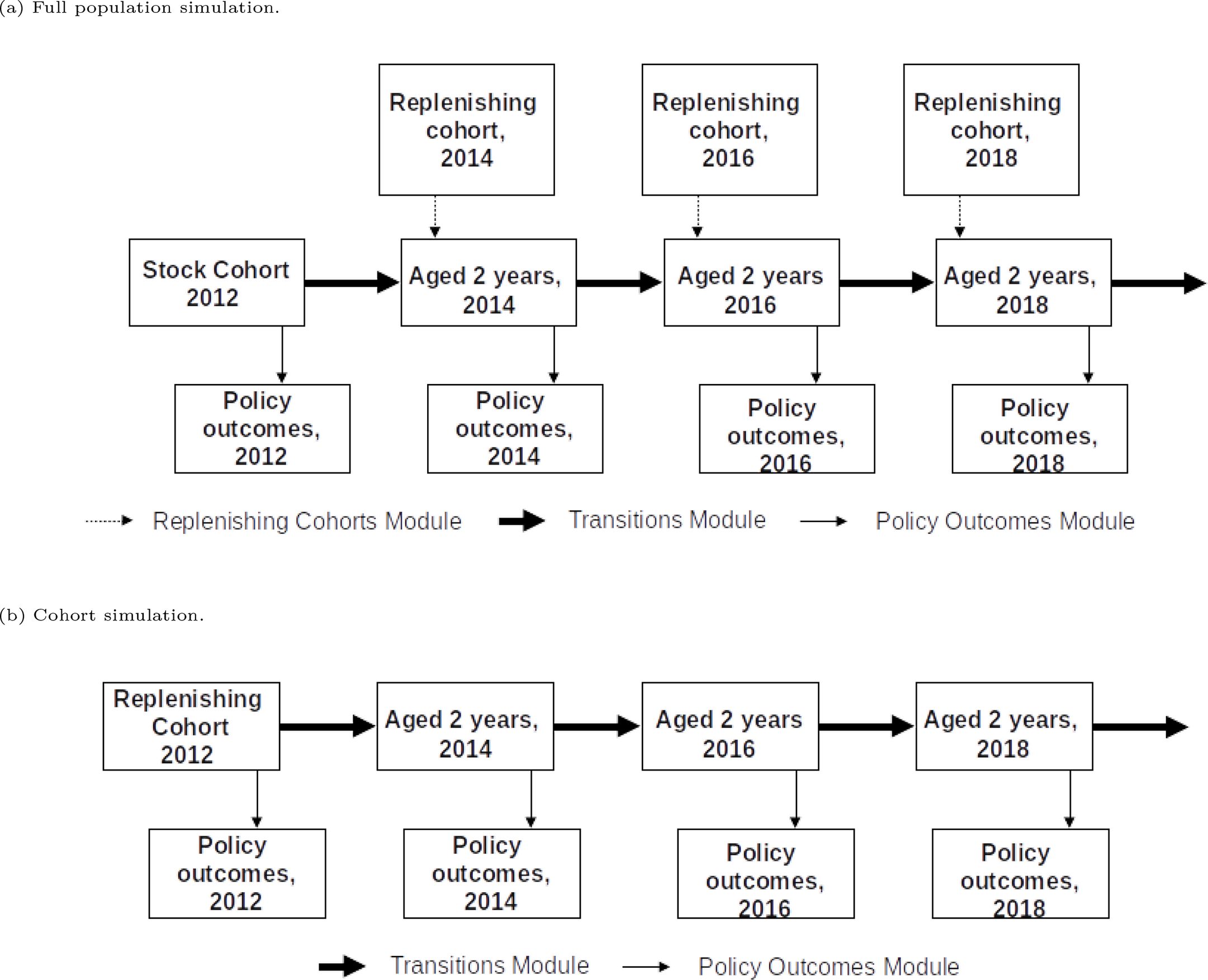

Structure of the FEM simulation.
3.3. Starting populations
Three separate data files are required to run the E-FEM: the stock, replenishing, and transition populations, all of which are generated from harmonised ELSA data. The stock population is produced from the whole sample of core respondents aged over 50 at wave 6 of ELSA (2012), and is the starting point for the population simulation. The replenishing population is derived from the stock population, where respondents aged 51 and 52 are extracted. The replenishing population is included at each new wave of the population simulation, to maintain the age distribution, but is also the starting point of the cohort simulation. The transition population contains all respondents from wave 2 onwards, and is used to estimate all of the statistical models that are used for ageing the simulants. Table 3 provides summary statistics on each population.
Summary statistics on key E-FEM populations.
| Characteristics | Stock | Replenishing | Transition | ||
|---|---|---|---|---|---|
| Year | 2012 | 2012 | 2004 - 2016 | ||
| Wave | 6 | 6 | 2 - 8 | ||
| Age, Mean (SD) | 66.2 (10.8) | 51.5 (0.5) | 66.1 (10.4) | ||
| Female % | 52.9 | 49.7 | 53.0 | ||
| BMI, Mean (SD) | 28.4 (5.4) | 27.8 (5.4) | 28.3 (5.3) | ||
| BMI Category (%) | |||||
| < 25 | 28.3 | 37.1 | 28.0 | ||
| ≥ 25 & < 30 | 38.8 | 34.8 | 39.9 | ||
| ≥ 30 | 33.0 | 28.1 | 32.1 | ||
| Smoking Status % | |||||
| Ever Smoked | 62.3 | 44.5 | 62.3 | ||
| Current Smoker | 13.6 | 13.7 | 14.3 | ||
| Education Level % | |||||
| Less than Secondary | 29.7 | 11.1 | 33.1 | ||
| Upper Secondary and Vocational | 59.9 | 64.1 | 65.7 | ||
| Tertiary | 10.4 | 24.8 | 11.2 | ||
| Disease Prevalence % (Incidence) | |||||
| Cancer | 9.8 | 2.9 | 9.0 (1.46) | ||
| Diabetes | 11.1 | 2.8 | 10.4 (1.34) | ||
| Heart Disease | 18.9 | 7.7 | 18.7 (2.57) | ||
| Stroke | 4.7 | 0.0 | 4.7 (0.85) | ||
| Lung Disease | 6.1 | 0.3 | 6.2 (0.87) | ||
| Hypertension | 41.8 | 20.4 | 42.0 (3.08) | ||
| Alzheimer’s | 0.35 | 0.0 | 0.32 (0.21) | ||
| Dementia | 1.25 | 0.27 | 1.12 (0.58) | ||
| High Cholesterol | 37.0 | 14.9 | 32.5 (3.92) | ||
The statistics for the replenishing population in Table 3 are based on 2012 data after re-weighting. The re-weighting step produces a copy of the replenishing population for each wave of the simulation with the cross-sectional weights modified to reflect projected changes in the future. The populations are re-weighted by age, sex, and education, which are all significant predictors for most outcomes. For example, there is an inverse relationship between smoking and education level, where individuals with low educational attainment are more likely to smoke. As smoking is related to a number of chronic diseases in the elderly, the risk therefore of developing these diseases is slightly higher in less educated groups. Over time the proportion of people with higher levels of education is rising, while the proportion of people who are less educated is falling. This will have a diminishing effect on the population level prevalence of these chronic diseases in the near future.
3.4. Imputation
One of the more significant challenges faced in the development of the E-FEM involves dealing with missing data in ELSA. Some variables are missing data for a significant proportion of records, including some key predictor variables such as highest educational qualification (20.9%) and BMI (19.2%). Both education and BMI are important predictors for a variety of outcomes, and so these variables were imputed before estimating transition models.
All other variables with missing data in the stock population undergo an imputation step during the preparation phase. This is because the model cannot run properly if input populations do not have complete data, as missing variables cannot be transitioned. As the replenishing population is derived from the stock, this imputation step ensures complete data in both starting populations. Table A1 in the appendix shows a comparison between the imputed and non-imputed stock populations, including the proportion of missing data for specific variables. No significant change in summary statistics is seen before and after imputation.
3.4.1. Education
Education level has been linked to health through a number of pathways. Higher-educated people are more likely to work full time in fulfilling employment, have higher levels of personal control and social support, and be less likely to take part in risk behaviours such as smoking and heavy drinking which are all significantly correlated with improved health (Ross and Wu, 1995). Education is therefore a key variable in the E-FEM, and imputed for respondents where it was missing.
During the preparation phase, an ordered probit model for education was estimated and used for imputing missing values during initialisation of the model. As predictors, the education model included demographics, marriage status, parents’ education, and spouse’s education (where applicable).
3.4.2. BMI
ELSA does not report BMI directly, but does report height and weight so that BMI can be calculated (which is handled by the harmonisation script from the Gateway to Global Aging). This information is collected as part of the nurse visit, which was originally only offered to ‘core sample members’ that were drawn from the Health Survey for England (HSE) and had an interview in person (that is not by proxy). They were also only carried out on odd numbered waves of the study, leaving missing data for even waves.
BMI is a significant predictor of a number of chronic diseases and mortality, as well as non-health-related outcomes such as labour-force participation. In order to effectively estimate transition models including BMI, we need information for every wave and as many respondents as possible. We therefore generated values for missing even waves using linear interpolation in Stata. As linear interpolation simply fills in the midpoint between known data points, transition models estimated from interpolated data showed that current BMI was wholly predicted by previous BMI. This did not mirror reality, and so we tested adding random noise to the interpolated values to assess if this looked more like observed data. For each interpolated data point, we added a sample from a normal distribution with mean 0 and standard deviation 0.05. When testing values for normal distribution, we compared the RMSE term of the BMI transition model with that in the US FEM, and stopped when the terms were roughly equal. Table A2 in the appendix shows a comparison of mean population BMI between raw and imputed ELSA data at each wave.
3.5. Transition probabilities
Transition probabilities were estimated from the transition panel dataset. Table 4 provides detailed information about these transition models, including the type of each response variable, the type of regression model used, and all the predictor variables included in each model. Briefly, the models for binary outcomes (such as disease incidence or mortality) use probits, ordered outcomes use ordered probits, non-ordered categorical outcomes use multinomial logit, and continuous outcomes use ordinary least squares. The choice of predictor variables to include in each model was based initially on previous literature, which were then refined iteratively, with the aim of producing parsimonious but well-specified models. The key demographic variables of age, sex, and education were included in every model. Some models are estimated for sub-groups of the population. For example, all individuals are included in the mortality model, only current smokers are included in the model that predicts smoking cessation, and only those who do not and have never had incident heart disease (since it is an absorbing state) are included in the heart disease model.
Information on transitioned variables in the model.
| Outcome | Variable Type | Regression Model | Predictors* | |||
|---|---|---|---|---|---|---|
| Health Status | Risk Behaviours | Economic Predictors | Demographics | |||
| Mortality incidence | Binary Absorbing | Probit | Cancer Diabetes Heart Disease Lung Disease Stroke Dementia |
Smoking | Age Sex Education |
|
| Cancer incidence | Binary Absorbing | Probit | BMI Smoking Alcohol Consumption |
Age Sex Ethnicity Education |
||
| Diabetes incidence | Binary Absorbing | Probit | Hypertension High Cholesterol |
BMI Physical Activity Alcohol Consumption |
Age Sex Ethnicity Education |
|
| Heart Disease incidence | Binary Absorbing | Probit | Diabetes Hypertension High Cholesterol |
BMI Smoking Physical Activity Alcohol Consumption |
Age Sex Ethnicity Education |
|
| Hypertension incidence | Binary Absorbing | Probit | High Cholesterol | BMI Smoking Alcohol Consumption Physical Activity |
Age Sex Ethnicity Education |
|
| Lung Disease incidence | Binary Absorbing | Probit | BMI Smoking |
Age Sex Ethnicity Education |
||
| Stroke incidence | Binary Absorbing | Probit | Hypertension Diabetes High Cholesterol |
BMI Smoking Alcohol Consumption |
Age Sex Ethnicity Education |
|
| High Cholesterol incidence | Binary Absorbing | Probit | BMI Smoking Physical Activity |
Age Sex Ethnicity Education |
||
| Dementia incidence | Binary Absorbing | Probit | Hypertension Stroke |
BMI Smoking |
Age Sex Ethnicity Education |
|
| Alzheimers incidence | Binary Absorbing | Probit | Hypertension Stroke |
BMI Smoking Alcohol Consumption |
Age Sex Ethnicity Education |
|
| Start/Stop Smoking | Binary | Probit | BMI | Age Sex Ethnicity Education |
||
| Alcohol Consumption | Binary | Probit | BMI Physical Activity |
Age Sex Ethnicity Education |
||
| BMI | Continuous | OLS | BMI Physical Activity |
Age Sex Ethnicity Education |
||
| Functional Limitations | Ordered | Oprobit | Stroke Dementia Alzheimers |
BMI Smoking |
Age Sex Ethnicity Education |
|
| Physical Activity | Ordered | Oprobit | Functional Limitations Physical Activity |
Age Sex Ethnicity Education |
||
| Labour Force Participation | Unordered | Mlogit | Functional Limitations | Age Sex Ethnicity Education |
||
-
*
All predictor variables are 2 year lag.
3.6. Outcomes
The FEM can produce both summary and detailed outputs for each scenario we choose to run. For detailed outputs, the state of the population at individual level is written to a new file for each repetition at every wave. Summary outputs are generated by pooling the results of each repetition, and calculating a number of summary statistics. For binary variables, the model reports the number of cases of an observation in the population, as well as the incidence between waves and the total prevalence. For continuous and ordinal variables, the model reports average values, as well as the total number (count), the total value, and quintile distributions.
Alongside the many variables which are tracked and transitioned throughout the simulation, there are also some outputs that we derive from these variables. For example, the model can be used to investigate life expectancy, as well as many related variables such as disability-free or disease-free life years.
4. Validation
In this section we validate a number of model outcomes. We focus on both internal validation (comparing predicted model outcomes with observed model inputs) and external validation by comparing model outputs with distributions seen in other datasets.
4.1. Internal validation
Internal validation of a microsimulation amounts to comparing the distribution of attributes between simulated outputs and the original data. In this work we employ three methods of internal validation; cross-validation, handover plots and Receiver Operating Characteristic (ROC) curves.
For cross-validation the original population was split in two, using only half of the population to estimate transition models. The remaining half was then simulated over the same time period as ELSA (2002 - 2016) using these models. We compared simulated outputs with ELSA data by performing t-tests, the results of which are provided in Tables A3. The handover plots and ROC curves will be presented in more detail below.
4.1.1. Handover plots
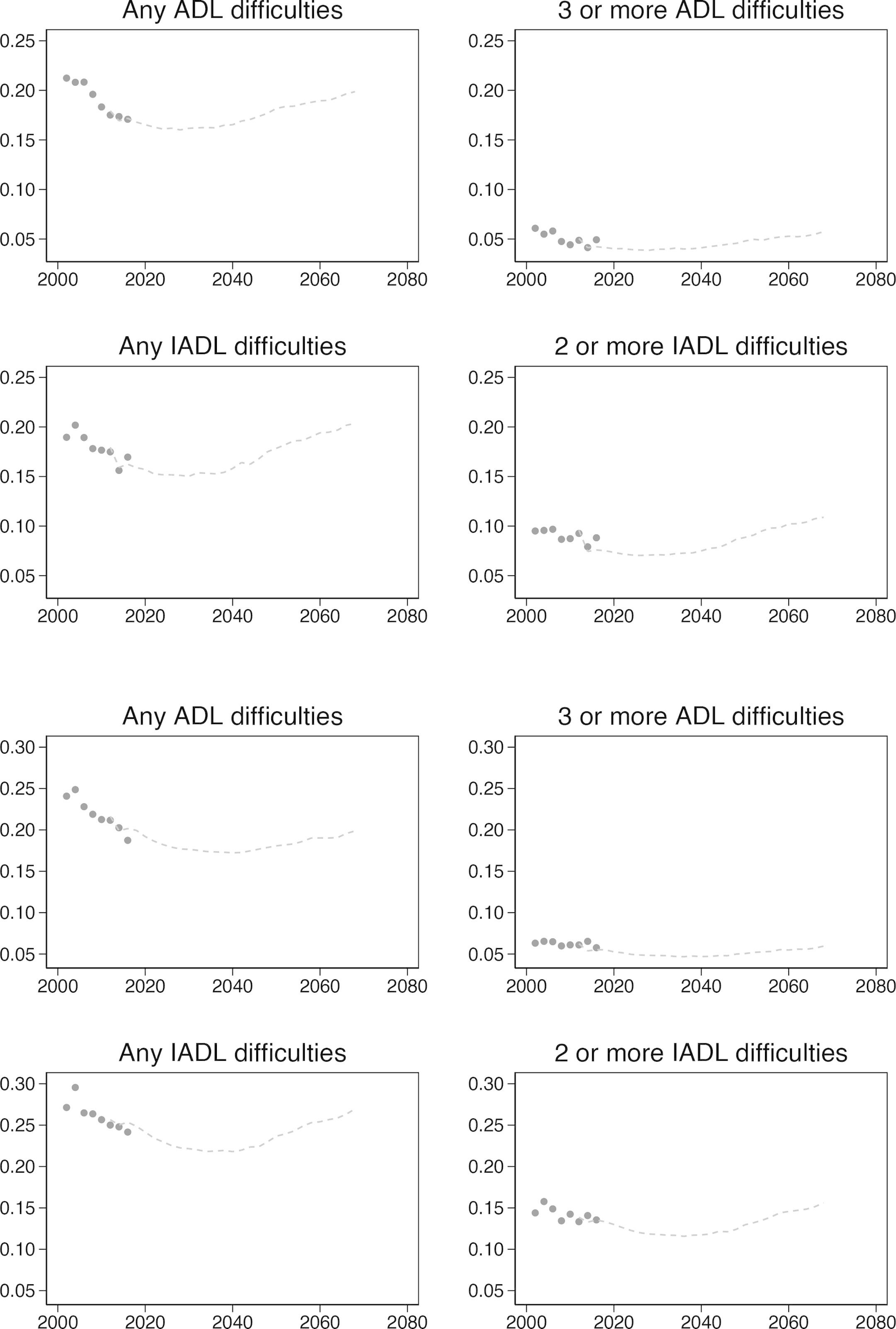
Handover plots are not a form of statistical validation, but rather a form of face validity. They give a quick visual indication that simulated outputs follow the same trend as the input data, and confirm that the model is behaving as expected. To generate these plots we estimated transitions using only data from waves 1-4 of ELSA, and produced a starting population based on respondents in wave 5 which was then simulated from wave 5 to 8. Combining these data, the plots in Figure 2 show the ’handover’ of chronic disease prevalence from ELSA to the simulation. For each chronic disease, the simulation continues a reasonable pattern from the original data, the predicted values are not noisy and the direction and magnitude of the trend appears sensible and in-line with expectations. Additional handover plots are provided in Figure A1.
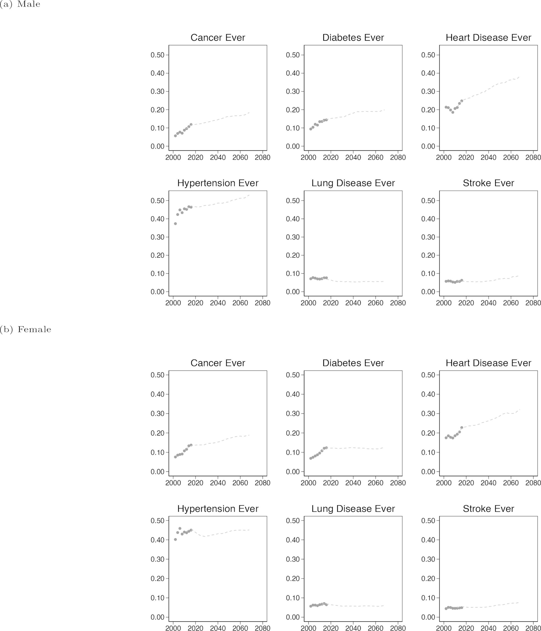

Handover plots for Chronic diseases by sex.
4.1.2. Receiver operating characteristic
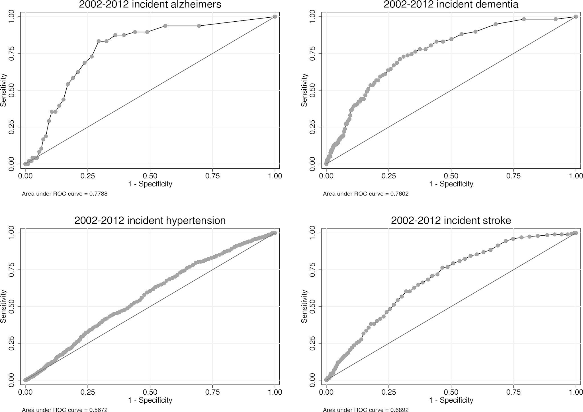
In order to investigate the efficacy of binary transitions in the model, we used Receiver Operating Characteristic (ROC) curves. First proposed by (Pandya et al., 2017) in a cardiovascular disease policy microsimulation, ROC curves are used to validate a binary classification, comparing the true-positive rate against the false-positive rate. The Area Under the Curve (AUC) relates to the accuracy of the prediction, with 1 being perfect classification when comparing simulated data to real, and 0.5 meaning the classification is no better than random.
For this analysis, we used the cross-validation population described above, where one half was used to estimate transition models and the remaining half used in the simulation. We simulated this population 500 times from 2002 - 2012 before pooling the results of each run to create a summary output file, which was then compared with ELSA data. The results of this analysis for key binary response variables are shown in Figure 3. In all cases the classification is better than random, and in some cases much better. For example, the AUC for predicting obesity (BMI > 30) and mortality is 0.85 and 0.83 respectively. Predicting chronic disease incidence is not as effective however, with AUCs ranging from 0.55 to 0.70. Additional ROC curves are provided in Figure A2.
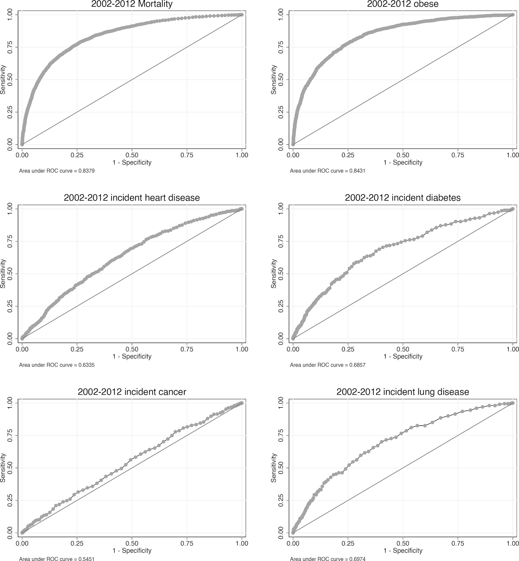

ROC curves for key binary response variables with a 10-year simulation horizon, from 2002 - 2012.
4.2. External validation
External validation involves comparing simulated outputs against independent external datasets. This is often more challenging than internal validation, as finding comparable datasets off the shelf is difficult since question wording and sample selection in surveys often differ. In the case of the E-FEM, chronic disease prevalence and incidence levels are projected into the future, starting in 2012. We can therefore use data published between 2012 and the present to validate the model over short time periods.
4.2.1. Comparison with age UK almanac reported disease prevalence
The Age UK almanac of disease profiles in later life (Melzer et al., 2015) is a collection of statistics on the prevalence of chronic diseases in elderly people, reported by sex and 5 year age group (over 60).
We ran a cohort simulation of the E-FEM for a 12-year period between 2004 to 2016 and compared the prevalence of a number of chronic diseases at the end of the simulation with those reported in the Age UK data. The results of the comparison can be seen in Figure 4 where the comparison is broken down by age group and sex. The graphs provide a good indication that the E-FEM is, on the whole, predicting chronic disease prevalence well (at least over a 12-year projection period) when compared to the results reported in the Age UK data. Unusual results in the 100 plus population from the E-FEM are most likely caused by a small sample size, as not many simulants survive to that age in the model. We were not able to compare the prevalence of cancer or heart disease in this validation as the Age UK definitions did not match those from ELSA. In the Age UK data cancer diagnosis relates to the previous 5 years only, whereas ELSA asks if the respondent has ever been diagnosed. Heart disease in the Age UK data was defined as one or more of a limited number of conditions, compared with ELSA which reports any heart condition as heart disease.
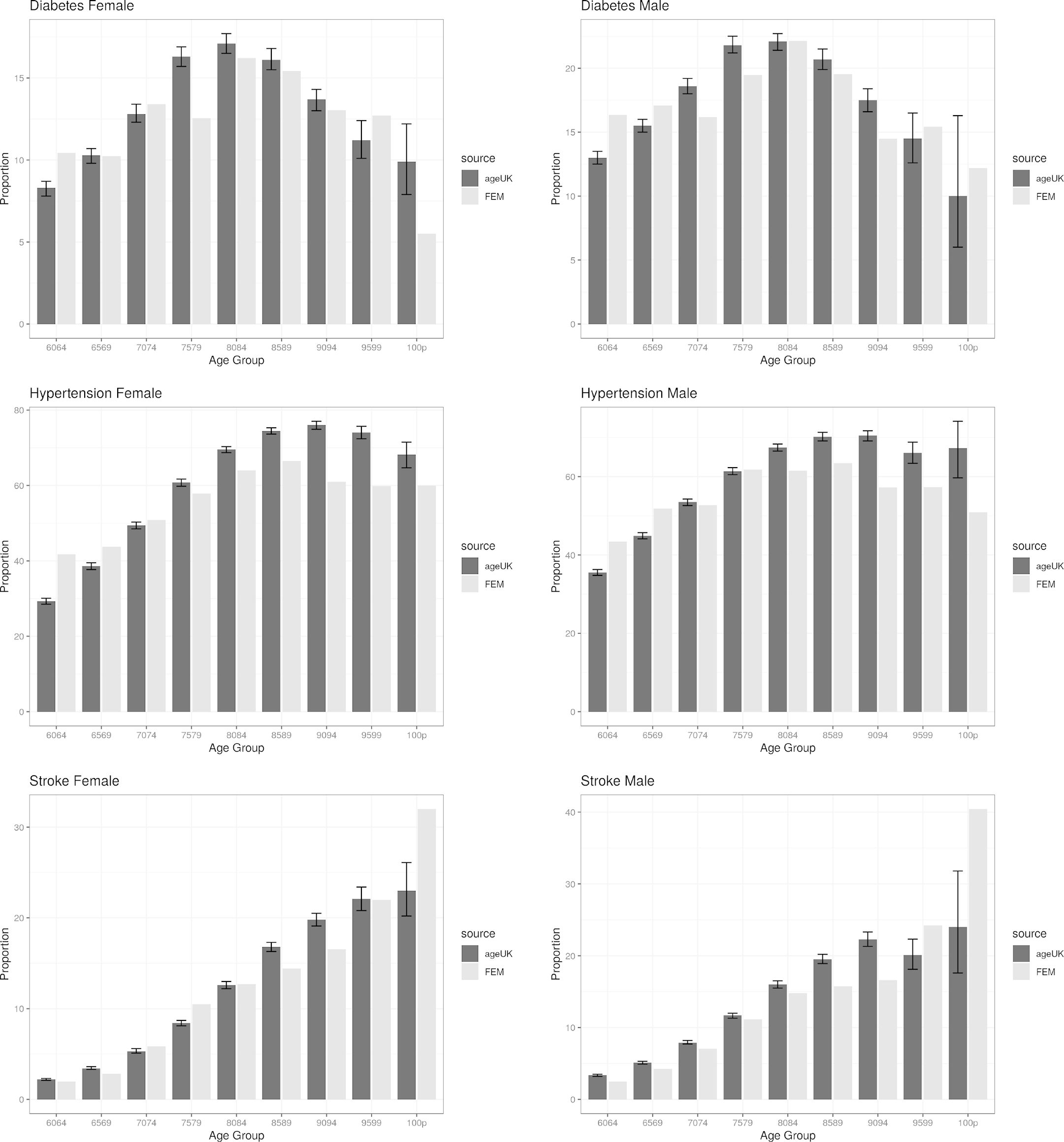

Chronic Disease prevalence comparisons by age group between FEM and AgeUK almanac of chronic disease in 2014. AgeUK figures include 95% confidence intervals.
4.2.2. Smoking
We ran the E-FEM model to 2018 and compared our estimates of smoking prevalence with data for the same year reported in a fact sheet published by Action on Smoking and Health (ASH) (ASH, 2020), a public health charity in the UK that works to eliminate the harm caused by tobacco, and produces statistical reports on smoking habits broken down by sex and age group. Figure 5 shows the comparison between simulated (E-FEM) and observed (ASH) data in 2018. In both age groups, the E-FEM is under-predicting the prevalence of current smokers by approximately 1-2 percentage points.
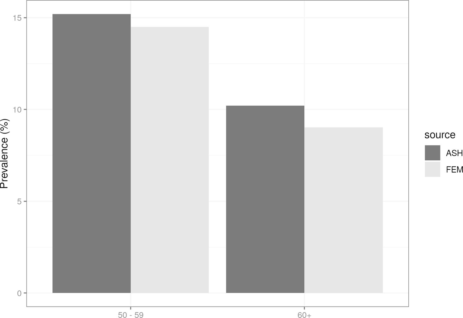
Smoking prevalence comparison by age group in 2018. Simulated data (starting in 2012) compared with prevalence statistics generated by the Action on Smoking and Health charity.
5. Results and discussion
The E-FEM provides a model capable of undertaking policy experimentation across a wide range of health outcomes. To illustrate the utility of the model, we present results from the baseline projections alongside two counterfactual scenarios, focused on heart disease and smoking. Heart disease provides an opportunity to demonstrate a change in outcomes where a chronic disease is directly impacted by model scenarios. Smoking provides an example where an intervention on a behaviour has an impact on health outcomes and survival.
5.1. Scenarios
For the baseline projections we ran both population and cohort simulations with no alterations. Both the stock and replenishing populations were included (where appropriate) without any modification, and ran for 56 years (28 waves) from 2012 to 2068. The scenario for heart disease was run as a whole population simulation in which nobody develops heart disease in the model. By removing heart disease completely, we can investigate its effect on mortality and disability and see how the removal of heart disease affects life expectancy and healthy life expectancy. The smoking scenario was run as a cohort simulation of people aged 51 and 52. In this scenario, smokers in the cohort immediately quit and do not start smoking again in the model. This way we can investigate the impact smoking has on chronic disease prevalence and mortality.
5.2. Heart disease
Heart disease in ELSA is a catch-all term which encapsulates a range of conditions that affect the heart’s structure and function and is part of a broader set of conditions which are known as Cardiovascular Disease (CVD). CVD is the leading cause of death worldwide, accounting for approximately 31% of all mortality (WHO, 5AD). In England, it is also one of the largest causes of premature mortality, with 33,812 people under the age of 75 dying from CVD in 2016 alone (Public Health England, 2AD). Mortality data from 2001 to 2016 in England has shown a long-term decline in the death rate from CVD, which is reported as one of the main reasons for the increase in life expectancy over this time period. Whilst mortality from CVD has decreased, morbidity has increased as people live longer with these conditions, which has increased the burden on health and social care. Public Health England (PHE) estimates that annual healthcare costs alone for CVD amount to an estimated £7.4 billion, whilst non-healthcare costs are much higher, estimated at £15.8 billion. CVD is one of the most significant targets for PHE, with numerous ongoing strategies for disease prevention. Table 5 shows the regression model used to estimate Heart Disease transitions in the E-FEM.
Parameter estimates for probit model of heart disease incidence.
| Heart Disease | |
|---|---|
| Male | 0.108*** |
| White | -0.0729 |
| Less than Secondary Education | -0.0642 |
| Higher or further education | 0.0194 |
| Lag of age spline, less than 65 | 0.0103 |
| Lag of age spline, 65 to 74 | 0.0262*** |
| Lag of age spline, more than 75 | 0.0182*** |
| Lag of BMI spline, less than 30 | 0.163 |
| Lag of BMI spline, more than 30 | 0.218 |
| Lag of ever smoker | 0.0259 |
| Lag of current smoker | 0.0264 |
| Lag of heavy smoker (>20 cigs/day) | 0.0836 |
| Lag of problem drinker (>12 drinks/week) | -0.0318 |
| Lag of doctor ever - Diabetes | 0.0520 |
| Lag of doctor ever - Hypertension | 0.163*** |
| Lag of doctor ever - High Cholesterol | 0.0659* |
| Lag of activity level - Low | 0.174** |
| Lag of activity level - Moderate | 0.0979* |
| Constant | -3.172*** |
| N | 22,333 |
| Pseudo R2 | 0.0335 |
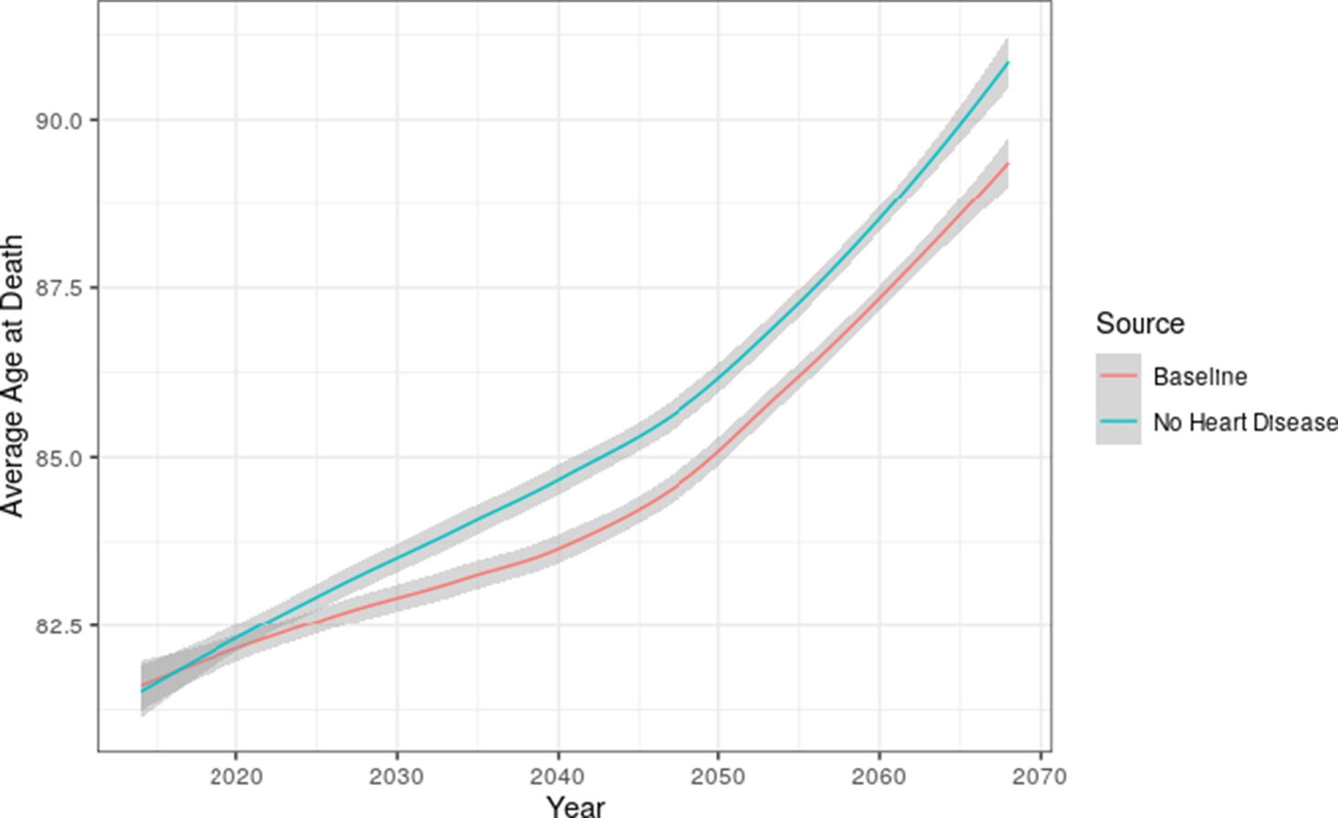
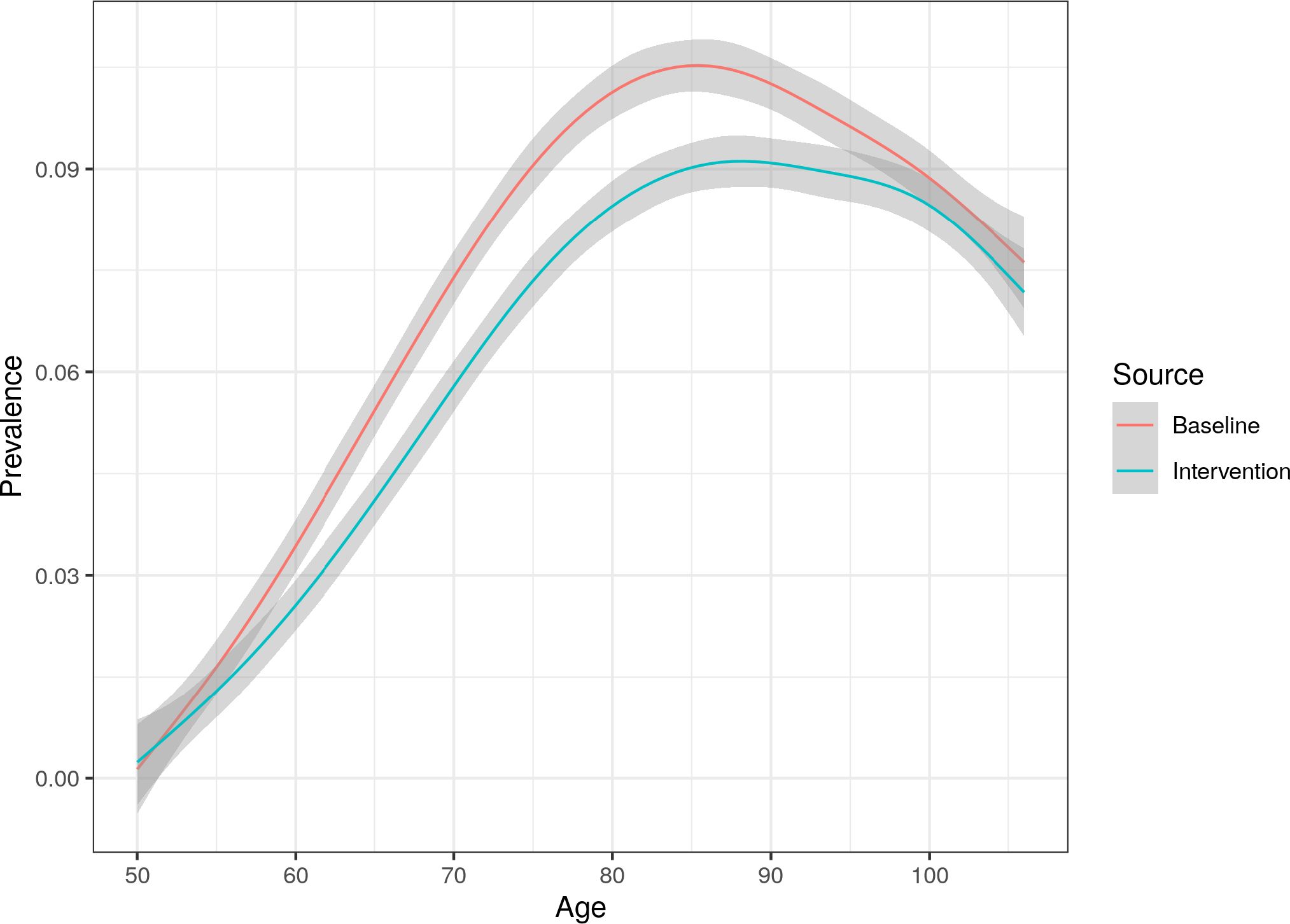
We used the E-FEM to investigate the total burden of disease in the elderly population by comparing the baseline projection to the counterfactual scenario in which nobody developed heart disease whilst in the model. The input populations were not modified in any way for this scenario, so any simulants in the stock or replenishing populations with heart disease were kept in the model. Figure 6 compares the average age at death between the baseline and intervention scenarios. There are improvements to overall survival in the intervention, with a significant difference emerging in 2028 of 0.5 years that increases to 1.2 years in 2050.

Average age at death comparison between baseline and no heart disease intervention. The shaded bands represent Monte Carlo confidence intervals.
5.3. Smoking
The impact of smoking on public health has been studied extensively, and the link between tobacco smoke and chronic health conditions is well understood (Newcomb and Carbone, 1992; Prasad et al., 2009; Al-Bashaireh et al., 2018). Various forms of tobacco control interventions have been attempted around the world, including mass media campaigns (Kuipers et al., 2018), advertising bans (Harris et al., 2006), price increases (Chaloupka et al., 2012), workplace and school smoking bans (Brown et al., 2009), and the addition of warning labels to packaging (Hammond et al., 2006). The outcomes of interest are usually health-related, however some studies have focused on Socio-Economic Status (SES), which has strong links to health. Table 6 shows the transition model for both starting and stopping smoking.
Parameter estimates for probit models of smoking initiation and cessation.
| Smoking | ||
|---|---|---|
| Started | Stopped | |
| Male | 0.112** | 0.0263 |
| White | 0.0228 | 0.257 |
| Less than Secondary education | 0.188*** | -0.106* |
| Higher or Further education | -0.154** | 0.215** |
| Lag of age spline, less than 65 | -0.00572 | 0.0188*** |
| Lag of age spline, 65 to 74 | -0.0186** | -0.00979 |
| Lag of age spline, more than 75 | -0.0289** | 0.0171 |
| Lag of BMI spline, less than 30 | -0.414* | 0.839*** |
| Lag of BMI spline, more than 30 | 0.25 | 0.0703 |
| Constant | -0.649 | -5.060*** |
| N | 41951 | 6157 |
| Pseudo R2 | 0.019 | 0.0129 |
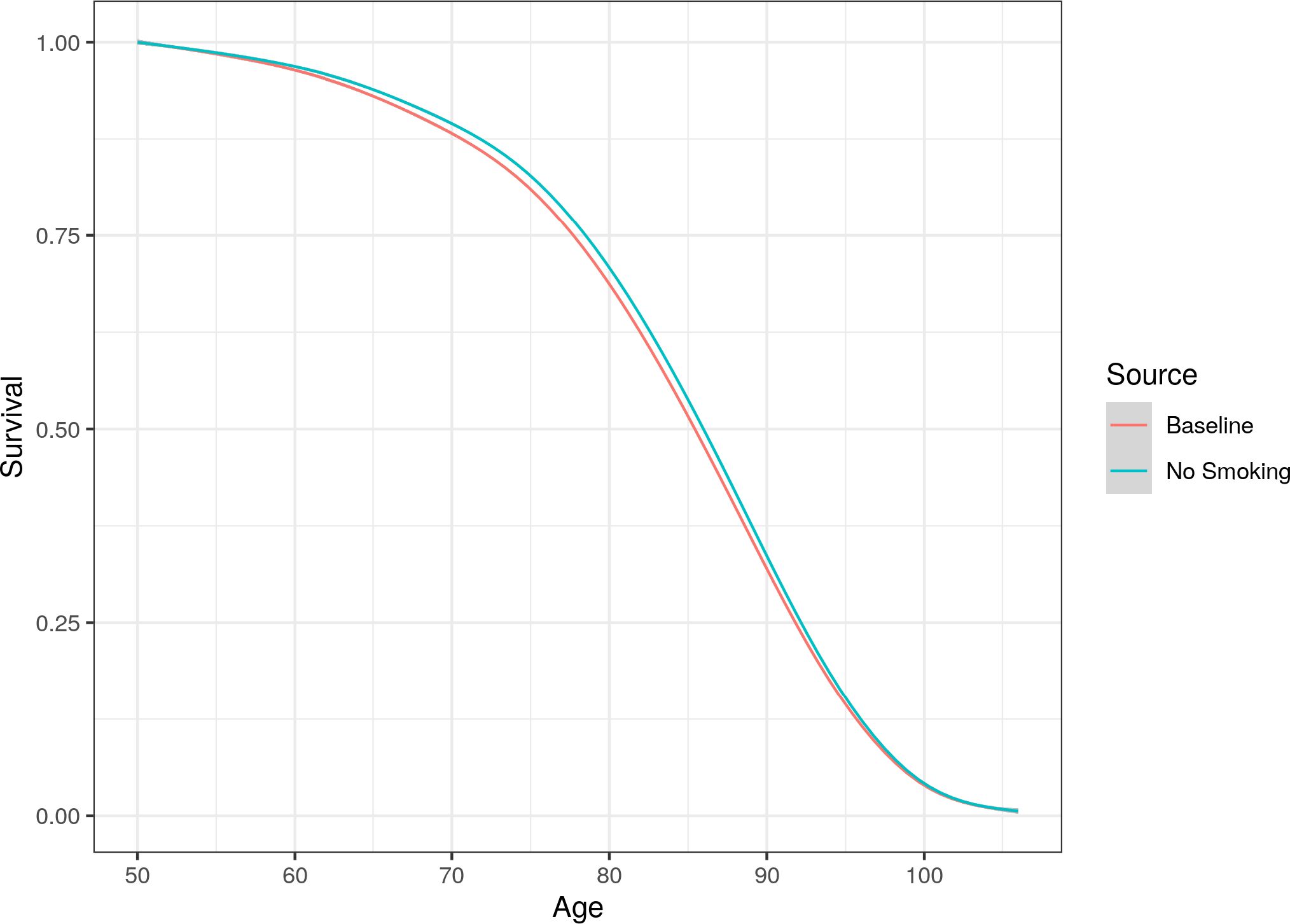
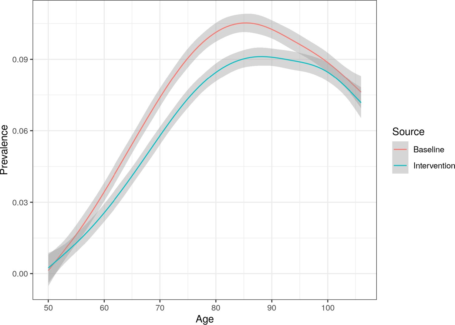
Figure 7 compares the average age at death in both the baseline and intervention case (where smokers in the cohort stop smoking and nobody starts smoking). This figure includes the whole population, including both smokers and non-smokers. Results show that average death age is only slightly higher in the no smoking scenario.
Whole population (including smokers and non-smokers) survival curve compared between the baseline and no smoking scenarios.
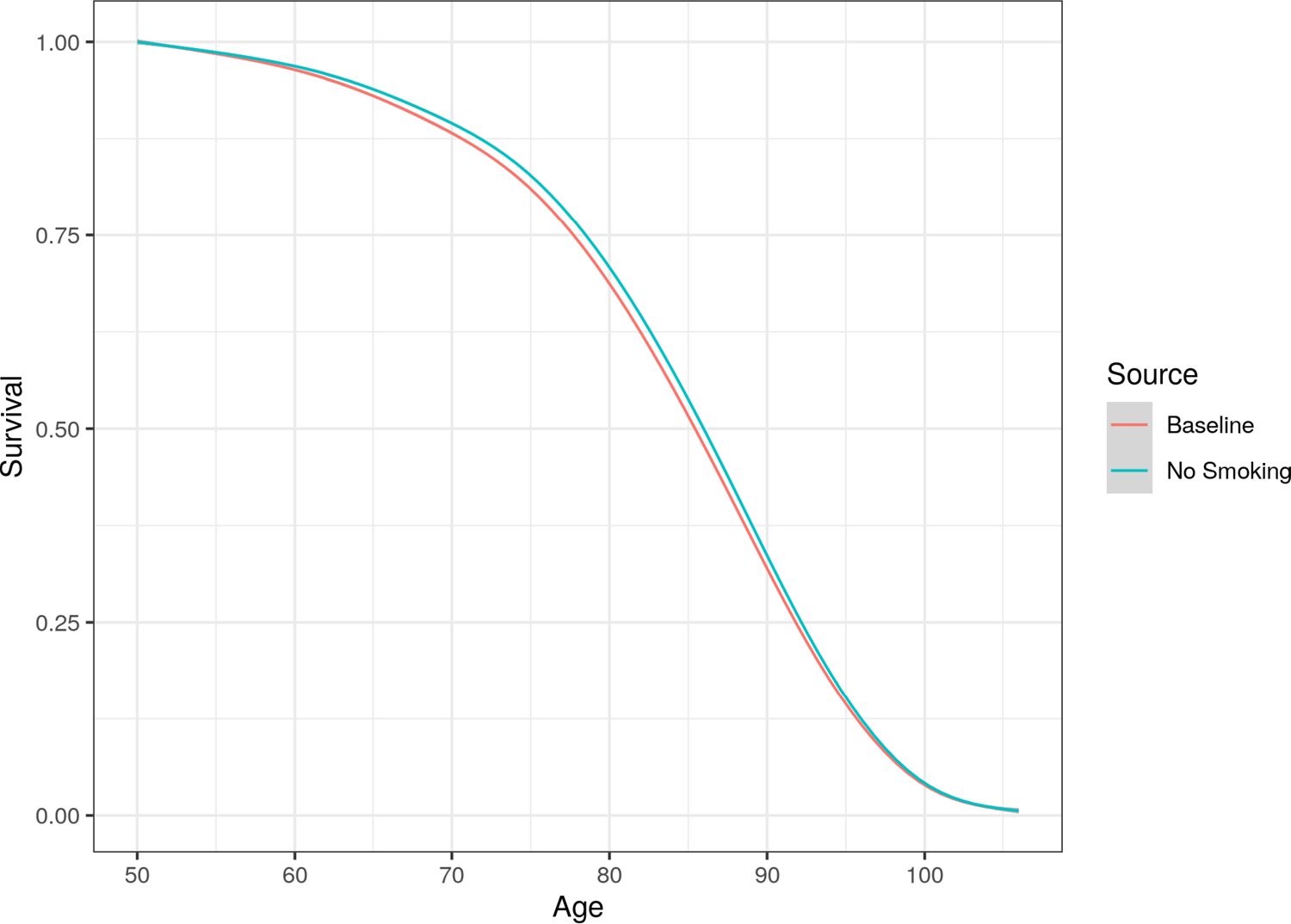
However, smoking does not just impact on mortality, but also has strong links to increased morbidity. This relationship is most obvious when looking at lung disease. Figure 8 plots the prevalence of lung disease in both the baseline and no smoking scenarios, once again including both smokers and non-smokers. There is a clear and significant difference between the scenarios, with prevalence of lung disease being approximately 1.5 percentage points lower after simulating both cohorts for 30 years. This difference is across the whole population, and not just smokers.
Whole population prevalence of lung disease comparison between the baseline and no smoking scenarios, with Monte Carlo confidence intervals.
5.3.1. Treatment on the treated
To further illustrate this link, we looked at the difference in life years and disability-free life years for smokers between the two scenarios, this time in a ’treatment on the treated’ analysis where only smokers are included. The results of this analysis are shown in Table 7. When looking at smokers only as opposed to the whole cohort, the improvement in life expectancy and healthy life expectancy is much more obvious. Smokers who quit at age 50 in this model live on average 7 years longer than if they did not. However, the improvement in disability-free life-expectancy is only approximately 4.5 years, suggesting that while those who quit live longer, only a proportion of this time equates to disability-free years.
Life year and disability-free life year comparison between baseline and no smoking scenario. This is a treatment on the treated analysis, so only including respondents that smoke.
| Scenario | Life Years | Disability-free Life Years |
|---|---|---|
| Baseline | 24.4 | 16.9 |
| Intervention | 31.4 | 21.4 |
We can run analyses by sub-population using the E-FEM. In the case of smoking we investigate how the intervention affects smokers by different levels of education. Table 8 shows the average increase in life years and disability-free life years by level of education. The largest overall improvement in life expectancy can be seen for the median educational level (level 2), with over eight years improvement. Those in the lowest education group (level 1) show the smallest average improvement in life years (5.5), as well as the lowest improvement in disability-free life years (3.4). These results suggest that other comorbidities disproportionately affect those with the lowest educational attainment, so even though intervention on a single attribute (smoking) delivers the substantial improvements in life expectancy, only a proportion of these extra years are disability free.
Average improvement in life years and disability-free life years between scenarios by highest level of education.
| Education Level | Life Years Improvement | Disability-free Life Years Improvement |
|---|---|---|
| 1 | 5.5 | 3.4 |
| 2 | 8.4 | 5.3 |
| 3 | 7.7 | 5.4 |
6. Conclusions
We set out with the aim of discussing the development of a dynamic microsimulation model for an ageing English population, the E-FEM. In this paper we have demonstrated how data from ELSA has been harmonised, cleaned and variables imputed to make it suitable for our model. Validation, both internal and external, demonstrates that the E-FEM is capable of accurately predicting health outcomes and disease states in to the future while results demonstrate that on a whole population and on a cohort the model can inform disease and mortality outcomes under counterfactual scenarios. We show results for a heart disease and a smoking intervention to demonstrate the type of experiments that can be run using the E-FEM but the model can be used to estimate a wide range of potential outcomes.
6.1. Limitations and future work
Developing and using a dynamic microsimulation like the E-FEM requires that some pragmatic decisions are made so as not to be overwhelmed by the complexity of the data, the model itself, and when interpreting outcomes. This can be summed up by considering the sources of uncertainty and bias which come in to play. The first arises from the data used as input. Limitations with ELSA have been discussed in this paper but in brief relate to bias and the representativeness of the data, missing values and changing data collection methods. The first of these have been mitigated somewhat by scaling to other data (Census, mid-year estimates and projections) and through imputation.
A second source of uncertainty arises from the estimation of the transition models. Further work to develop policy specific-models using the E-FEM could utilise non-parametric bootstrapping or other methods to improve these models. Third, that the E-FEM is a Monte Carlo simulation means that outputs are inherently uncertain. We have generally used the average result from 100 runs in our results, and have quantified this uncertainty using confidence intervals where possible.
Fourth, and most difficult to deal with, is that the future is inherently uncertain. Trends in predictors that are important for estimating transitions within the model, such as risk behaviours (smoking, drinking, etc.) are very difficult to predict. Future development of the model could deal with these in a similar way to how we currently deal with changes in educational attainment. Experimentation with trends in risk behaviours and demographic change could be used to modify future populations.
6.1.1. Prediction of cancer incidence
Special mention must be given to the prediction of cancer, which as shown in Figure 3 is not performing much better than chance when compared with original ELSA data. There are a couple of possible contributing factors at play that mean cancer prevalence and mortality may not wholly be captured by ELSA, as well as other reasons why cancer may be difficult to predict from this data. Firstly, the time between diagnosis and death is often short for cancer, which gets progressively worse with age. For example in lung cancer, the 1-year survival rate for someone diagnosed between ages 55-64 is 44.7%, whereas the same diagnosis between ages 75-99 has a 1-year survival rate of 32.0% (ONS, 2019b). There is therefore a significant chance that a respondent diagnosed with cancer between waves may not survive to the next wave. Secondly, cancer is one of the leading reasons for the need for palliative care. As previously stated, respondents who move into assisted living facilities (including palliative care) are given an analysis weight of zero, effectively removing them from our analyses. Thirdly, current predictors taken from ELSA (for example BMI, smoking status) may not be adequate for the prediction of cancer in this case. Further information such as family history, pack-years for smokers, or other environmental exposures may be necessary to improve the model. Also given that different types of cancer can have very specific behavioural and genetic risks, it may be inadequate to predict incidence of all types of cancer with a single set of predictor variables. Finally, cancer could be more of a ’random shock’ than other diseases, meaning prediction of it is more difficult than other diseases even with perfect data.
6.1.2. Summary
This paper has provided an overview of the development of the E-FEM and sought to demonstrate its utility and validity as a model for undertaking policy analysis related to an ageing English population. We set out the basis for further work which will address policy questions which are specifically pertinent to this ageing population. It also marks further expansion of the FEM model developed for the US which has subsequently been adapted and applied to other countries. This will provide an opportunity to undertake cross-country comparisons with the English population represented in our work.
The potential applications of this model are broad, as evidenced by the history of FEM models in the United States and around the world. Moving forward, we intend to use the E-FEM to assess the burden of chronic disease, evaluate the impact of early life experiences on later-life health, investigate the relationship between socio-economic factors and the quality and quantity of life, and quantify the potential impact for interventions targeting key risk factors.
Footnotes
Appendix
Imputation

Handover plots for ADLs and IADLs.

Receiver Operating Characteristic curves.
Summary statistics for raw and imputed stock populations, including the percentage of missing data where applicable.
| Characteristics | Raw Stock | Imputed | Missing (%) |
|---|---|---|---|
| Age, Mean (SD) | 66.5 (10.8) | 66.2 (10.8) | 0 |
| Female (%) | 52.9 | 52.9 | 0 |
| BMI, Mean (SD) | 28.4 (5.4) | 28.4 (5.4) | 19.2 |
| BMI Category (%) | |||
| < 25 | 28.3 | 28.3 | - |
| ≥ 25 & < 30 | 42.2 | 42.2 | - |
| ≥ 30 | 29.5 | 29.5 | - |
| Smoking Status (%) | |||
| Ever Smoked | 62.5 | 62.3 | 1.83 |
| Current Smoker | 12.2 | 13.6 | 0.05 |
| Education Level (%) | 20.9 | ||
| Less than Secondary | 38.6 | 38.6 | - |
| Upper Secondary and Vocational | 48.0 | 47.9 | - |
| Some University or more | 13.5 | 13.5 | - |
| Initial Disease Prevalence (%) | |||
| Cancer | 9.8 | 9.8 | 0.009 |
| Diabetes | 11.1 | 11.1 | 0.009 |
| Heart Disease | 18.9 | 18.9 | 0.009 |
BMI
Raw vs imputed BMI mean and standard deviation at each wave of ELSA.
| Wave | Raw BMI | Imputed BMI |
|---|---|---|
| 1 | - | 28.0 (5.3) |
| 2 | 28.0 (4.9) | 28.0 (5.0) |
| 3 | - | 28.2 (5.2) |
| 4 | 28.3 (5.4) | 28.4 (5.4) |
| 5 | - | 28.4 (5.4) |
| 6 | 28.4 (5.3) | 28.4 (5.4) |
| 7 | - | 28.4 (5.4) |
| 8 | 28.3 (5.5) | 28.3 (5.5) |
T-test results for health outcomes.
| Variable | FEM 3 | ELSA 3 | P value 3 | FEM 5 | ELSA 5 | P value 5 | FEM 8 | ELSA 8 | P value 8 |
|---|---|---|---|---|---|---|---|---|---|
| Alzheimers | 0.0067 | 0.00325 | 0.00076 | 0.0103 | 0.00404 | 0 | 0.0178 | 0.0119 | 0.0204 |
| Any ADLs | 0.184 | 0.213 | 0 | 0.199 | 0.234 | 0 | 0.241 | 0.225 | 0.0938 |
| Any IADLs | 0.204 | 0.222 | 0.012 | 0.230 | 0.255 | 0.00292 | 0.268 | 0.266 | 0.839 |
| Cancer | 0.1 | 0.0863 | 0.00448 | 0.130 | 0.119 | 0.0836 | 0.176 | 0.164 | 0.182 |
| Dementia | 0.0159 | 0.0102 | 0.00156 | 0.0226 | 0.0194 | 0.24 | 0.0324 | 0.164 | 0.0214 |
| Diabetes | 0.109 | 0.0937 | 0.00275 | 0.132 | 0.128 | 0.571 | 0.164 | 0.151 | 0.125 |
| Heart disease | 0.220 | 0.175 | 0 | 0.26 | 0.222 | 0 | 0.328 | 0.29 | 0.00031 |
| Hypertension | 0.453 | 0.448 | 0.555 | 0.491 | 0.506 | 0.115 | 0.549 | 0.538 | 0.381 |
| Lung disease | 0.0836 | 0.0719 | 0.00989 | 0.0957 | 0.0863 | 0.0857 | 0.111 | 0.0898 | 0.00167 |
| Stroke | 0.0558 | 0.0504 | 0.156 | 0.0667 | 0.06743 | 0.875 | 0.082 | 0.089 | 0.289 |
t-test results for economic outcomes.
| Variable | FEM 3 | ELSA 3 | P value 3 | FEM 5 | ELSA 5 | P value 5 | FEM 8 | ELSA 8 | P value 8 |
|---|---|---|---|---|---|---|---|---|---|
| Employed | 0.284 | 0.285 | 0.906 | 0.194 | 0.179 | 0.0412 | 0.0809 | 0.0842 | 0.606 |
| Unemployed | 0.00102 | 0.00662 | 0.0132 | 0.00519 | 0.00675 | 0.321 | 0.00137 | 0.00092 | 0.529 |
| Retired/Disabled | 0.706 | 0.707 | 0.0.84 | 0.801 | 0.811 | 0.167 | 0.918 | 0.912 | 0.411 |
t-test results for risk behaviours.
| Variable | FEM 3 | ELSA 3 | P value 3 | FEM 5 | ELSA 5 | P value 5 | FEM 8 | ELSA 8 | P value 8 |
|---|---|---|---|---|---|---|---|---|---|
| BMI* | 28.4 | 28.0 | 0.0014 | ||||||
| Drinks Alcohol | 0.866 | 0.874 | 0.205 | 0.859 | 0.851 | 0.239 | 0.844 | 0.839 | 0.552 |
| Problem Drinker | 0.12 | 0 | 0 | 0.122 | 0.127 | 0.487 | 0.109 | 0.113 | 0.567 |
| Activity - Low | 0.0907 | 0.101 | 0.0426 | 0.099 | 0.13 | 0 | 0.112 | 0.129 | 0.0304 |
| Activity - Moderate | 0.164 | 0.162 | 0.739 | 0.168 | 0.181 | 0.0775 | 0.183 | 0.201 | 0.0508 |
| Activity - High | 0.745 | 0.736 | 0.231 | 0.733 | 0.689 | 0 | 0.706 | 0.669 | 0.00097 |
| Smoke Now | 0.132 | 0.143 | 0.0678 | 0.106 | 0.116 | 0.106 | 0.076 | 0.0708 | 0.391 |
| Smoke Ever | 0.637 | 0.628 | 0.279 | 0.639 | 0.648 | 0.322 | 0.638 | 0.658 | 0.0646 |
| Heavy Smoker | 0.0234 | 0.0297 | 0.906 | 0.0214 | 0.0229 | 0.595 | 0.0128 | 0.0136 | 0.761 |
-
*
ELSA only reports BMI information for even waves.
t-test results for mortality.
| Variable | FEM 3 | ELSA 3 | P value 3 | FEM 5 | ELSA 5 | P value 5 | FEM 8 | ELSA 8* | P value 8 |
|---|---|---|---|---|---|---|---|---|---|
| Died | 0.0294 | 0.0412 | 0.00033 | 0.0435 | 0.0602 | 0 | 0.0596 | 0 | 0 |
-
*
End of life interviews are only reporte for waves 2-6 (excluding wave 5). There is therefore no mortality informationfor waves 7 or 8.
References
-
1
The Effect of Tobacco Smoking on Musculoskeletal Health: A Systematic ReviewJournal of Environmental and Public Health 2018 :4184190.https://doi.org/10.1155/2018/4184190
- 2
-
3
The future of the elderly population health status: Filling a knowledge gapHealth Economics 30 Suppl 1 :1.https://doi.org/10.1002/hec.4258
-
4
Comparison of Ageing in Europe and Asia: Refining the Prospective Age Approach with a Cross-Country Perspective, Netherlands Interdisciplinary Demographic InstituteComparison of Ageing in Europe and Asia: Refining the Prospective Age Approach with a Cross-Country Perspective, Netherlands Interdisciplinary Demographic Institute.
-
5
English Longitudinal Study of Ageing: Waves 0-9, 1998-2019UK Data Service.https://doi.org/10.5255/UKDA-SN-5050-24
-
6
Attrition and health in ageing studies: Evidence from ELSA and HRSLongitudinal and Life Course Studies 2 :2.https://doi.org/10.14301/llcs.v2i2.115
-
7
A longitudinal study of policy effect (smoke-free legislation) on smoking norms: ITC Scotland/United KingdomNicotine & Tobacco Research 11 :924–932.https://doi.org/10.1093/ntr/ntp087
- 8
-
9
Tobacco taxes as a tobacco control strategyTobacco Control 21 :172–180.https://doi.org/10.1136/tobaccocontrol-2011-050417
-
10
Forecasting Trends in Disability in a Super-Aging Society: Adapting the Future Elderly Model to JapanJournal of the Economics of Ageing 8 :42–51.https://doi.org/10.1016/j.jeoa.2016.06.001
-
11
The Long-Term Impact of Functional Disability on Hospitalization Spending in SingaporeJournal of the Economics of Ageing 14 :100193.https://doi.org/10.1016/j.jeoa.2019.02.002
-
12
LIAM2: a New Open Source Development Tool for Discrete-Time Dynamic Microsimulation ModelsJournal of Artificial Societies and Social Simulation 17 :1–9.https://doi.org/10.18564/jasss.2574
- 13
-
14
Consequences of health trends and medical innovation for the future elderly: When demographic trends temper the optimism of biomedical advances, how will tomorrow’s elderly fareHealth Affairs 24 :W5–R5.
-
15
Health status and medical treatment of the future elderlySanta Monica, CA: RAND Corporatio.
-
16
Projecting diabetes prevalence among Mexicans aged 50 years and older: the Future Elderly Model-Mexico (FEM-Mexico)BMJ Open 7 :e017330.https://doi.org/10.1136/bmjopen-2017-017330
-
17
The MISCAN simulation program for the evaluation of screening for diseaseComputer Methods and Programs in Biomedicine 20 :79–93.https://doi.org/10.1016/0169-2607(85)90048-3
-
18
Effectiveness of cigarette warning labels in informing smokers about the risks of smoking: findings from the International Tobacco Control (ITC) Four Country SurveyTobacco Control 15 Suppl 3 :iii19–25.https://doi.org/10.1136/tc.2005.012294
-
19
Effects of the 2003 advertising/promotion ban in the United Kingdom on awareness of tobacco marketing: findings from the International Tobacco Control (ITC) Four Country SurveyTobacco Control 15 Suppl 3 :iii26–33.https://doi.org/10.1136/tc.2005.013110
-
20
The Population Health Model (POHEM): an overview of rationale, methods and applicationsPopulation Health Metrics 13 :1–12.https://doi.org/10.1186/s12963-015-0057-x
-
21
Towards a computerized demographic microsimulation model for Egypt: experimentation of POPSIM: 1The Egyptian Population and Family Planning Review 5 :153–166.
-
22
Smoking, life expectancy, and chronic disease in South Korea, Singapore, and the United States: A microsimulation modelHealth Economics 30 Suppl 1 :1.https://doi.org/10.1002/hec.3978
-
23
Associations between tobacco control mass media campaign expenditure and smoking prevalence and quitting in england: a time series analysisTobacco Control 27 :455–462.https://doi.org/10.1136/tobaccocontrol-2017-053662
-
24
Predicting quantity and quality of life with the future elderly modelHealth Economics 30 :52–79.https://doi.org/10.1002/hec.4169
-
25
The impacts of international migration on the uk’s ethnic populationsJournal of Ethnic and Migration Studies 46 :177–199.https://doi.org/10.1080/1369183X.2019.1577726
-
26
Variation in adenoma detection rate and the lifetime benefits and cost of colorectal cancer screening: a microsimulation modelJAMA 313 :2349–2358.
-
27
The Ageuk Almanac of Disease Profiles in Later Life, UK, Ageing Research Group, University of ExeterThe Ageuk Almanac of Disease Profiles in Later Life, UK, Ageing Research Group, University of Exeter.
-
28
Differences in health between americans and western europeans: Effects on longevity and public financeSocial Science & Medicine 73 :254–263.
-
29
Fecundability Differentials among Acceptors and Non-Acceptors of Family Planning: A Simulation Experiment,’’ Ph.D. Dissertation, CiteseerFecundability Differentials among Acceptors and Non-Acceptors of Family Planning: A Simulation Experiment,’’ Ph.D. Dissertation, Citeseer.
-
30
The current and potential health benefits of the national health service health check cardiovascular disease prevention programme in england: a microsimulation studyPLoS Medicine 15 :e1002517.
-
31
The health consequences of smoking: cancerMedical Clinics of North America 76 :305–331.https://doi.org/10.1016/S0025-7125(16)30355-8
- 32
- 33
-
34
Validation of a cardiovascular disease policy microsimulation model using both survival and receiver operating characteristic curvesMedical Decision Making 37 :802–814.https://doi.org/10.1177/0272989X17706081
-
35
Smoking and cardiovascular health: a review of the epidemiology, pathogenesis, prevention and control of tobaccoDian Journal of Medical Sciences 63 11 :520–533.
- 36
- 37
-
38
Dynamic microsimulation models for health outcomes: a reviewMedical Decision Making 31 :10–18.
-
39
Thesis (PhDThesis (PhD, A Microsimulation Model of Human Fertility: Theory and Applications to the Yoruba of Western Nigeria.
-
40
A brief, global history of microsimulation models in health: past applications, lessons learned and future directionsT. J. Microsimulation 11 :97–142.
-
41
Stata Statistical Software: Release 17. College Station, Tx: Statacorp LlcStata Statistical Software: Release 17. College Station, Tx: Statacorp Llc.
-
42
Modeling the clinical and economic implications of obesity using microsimulationJournal of Medical Economics 18 :886–897.
-
43
Predicting the effects of mass-screening for disease—a simulation approachEuropean Journal of Operational Research 6 :399–409.
- 44
-
45
Valuing Innovations in Cancer TreatmentJournal of Clinical Oncology 37 :e18176–e18176.
Article and author information
Author details
Funding
This work was supported by Wave 1 of The UKRI Strategic Priorities Fund under the EPSRC Grant EP/T001569/1, particularly the ‘Digital Twins: Urban Analytics’ theme within that grant and The Alan Turing Institute.
Acknowledgements
The English Longitudinal Study of Ageing was developed by a team of researchers based at University College London, NatCen Social Research, the Institute for Fiscal Studies, the University of Manchester and the University of East Anglia. The data were collected by NatCen Social Research. The funding is currently provided by the National Institute on Aging in the US, and a consortium of UK government departments coordinated by the National Institute for Health Research. Funding has also been received by the Economic and Social Research Council. This analysis uses data or information from the Harmonized English Longitudinal Study of Ageing dataset and Codebook, Version E as of April 2017 developed by the Gateway to Global Aging Data. The development of the Harmonized English Longitudinal Study of Ageing was funded by the National Institute on Aging (R01 AG030153, RC2 AG036619, 1R03AG043052). For more information, please refer to www.g2aging.org.
Publication history
- Version of Record published: December 31, 2021 (version 1)
Copyright
© 2021, Archer
This article is distributed under the terms of the Creative Commons Attribution License, which permits unrestricted use and redistribution provided that the original author and source are credited.