Simulations of Policy Responses During the COVID-19 Crisis in Argentina: Effects on Socioeconomic Indicators
- Center for Distributive, Labor and Social Studies (CEDLAS). Institute of Economic Research of the Faculty of Economic Sciences at the National University of La Plata (UNLP), Argentina
Abstract
This paper simulates the effects of policy responses to the COVID-19 pandemic on household income and employment in Argentina, using household survey data and administrative data on employment and wages by economic sectors. The paper also includes a gender and age group analysis. The results indicate that during the COVID-19 crisis, household income decreased. This welfare loss was nonlinear along the income distribution, with the lowest income earners suffering the most due to relatively higher informality at the bottom of the income distribution. The policy responses seem to ameliorate by around one-third what the average drop in household income, and prevented major increases in poverty and inequality.
1. Introduction and background
As in most countries, the COVID-19 pandemic has caused a severe crisis in Argentina. The preventive and mandatory social isolation policy (ASPO in Spanish), established by the national government on March 20, 2020, had the primary objective of immobilizing the population to prevent further transmission and to gain time to prepare the health system for the care of patients. The ASPO had been extended for more than 200 days, being one of the longest isolation periods in the world and greatly affecting the country’s economic activity. According to the National Institute of Statistics and Census (INDEC) of Argentina, economic activity fell by 25 percent in April and by 20 percent in May (compared to the same months of 2019). While many productive and essential services continued normally (e.g., food production, health services), other less essential services were significantly reduced (e.g., transportation, construction, domestic services). Those that required a physical presence in the workplace (e.g., manufacturing, construction) were also restricted, and others were directly suspended (e.g., tourism, recreation). In addition, some activities were adapted and carried out remotely (e.g., many professional services, education). This reduction in economic activity has put the job stability of many people at risk, affecting their income levels and deteriorating social indicators.
In this context, the Argentine government has implemented a series of economic policy responses to face the crisis. To guarantee access to food and to sustain the income of less well-off sectors, it established Emergency Family Income (IFE in Spanish). This was an exceptional monthly payment of $10,000 pesos (around US$120, about 60 percent of the minimum wage) during April, June, and August 2020 to unemployed people, informal workers, low-income self-employed workers, and domestic workers. The social protection system was also reinforced. Beneficiaries of cash transfer programs (e.g., holders of the Universal Child Allowance (AUH) and Universal Allowance for Pregnancy (AUE)) received a bonus payment, and retirees and pensioners received an extra payment.1 This package of measures had an estimated fiscal cost of approximately four points of GDP, and had been in place from the beginning of the crisis until the end of 2020 for activities that were affected by the crisis.2
This paper simulates the effects of policy responses to the COVID-19 pandemic on households’ employment and income distribution, using household survey and administrative data on employment and wages by economic sectors. The underlying hypothesis is that the COVID-19 crisis strongly deteriorated the Argentine economy and household welfare, but the implemented public policies collaborated to counteract (at least partially) these negative effects. To examine this hypothesis, we analyze the impact of the COVID-19 crisis on households’ income, unemployment, poverty, and inequality. Women may have been the most affected by the crisis: the most affected economic sectors are mainly occupied by women (e.g. domestic service) and school closures may have forced them to childcare at home. We then explore heterogeneous effects by gender and age groups. For this purpose, we simulate impacts on welfare at the household level using household survey data, administrative data on employment and wages by economic sectors, and government cash transfers.
We start by considering two different scenarios. We first characterize a pre-COVID-19 scenario in terms of socioeconomic indicators using microdata from Argentina’s household survey corresponding to the first quarter of 2020. We then simulate the effects on unemployment and household income for three quarters after the beginning of the pandemic (i.e., post-COVID-19 scenarios).3 To this aim, we use the latest available figures on the evolution of economic activity and past changes on employment and wages by sector. All scenarios also include public assistance (i.e., policy responses through cash transfers), in line with what the Argentine government is doing to mitigate the crisis, to get a general sense of how effective these policies were in counteracting those effects.
The results indicate that during the COVID-19 crisis, households would have seen their income decline by about 6 percent without the policy responses. This reduction was nonlinear along the income distribution, with the lowest income earners suffering the most in relative terms. This is strongly related to the relatively higher informality at the bottom of the income distribution. The greater negative effects of the pandemic in the less well-off part of the income distribution are in line with results from Bonavida and Gasparini (2020). Furthermore, we find suggestive evidence that the impact was not homogeneous by gender: on average, the employment rate fell more among women than men (–23 percent versus –20.8 percent compared to the second and first quarters of 2020). In early working ages (18–24) the differences are very significant: the fall in the employment rate was 63 percent for men and 80 percent for women. These differences become more pronounced when considering the presence of children. For example, for the age group 18–24, the contraction in employment for men with children was close to 57 percent, while it was 82 percent for women with children. In the 25–40 age group, the falls were 18 percent for men with children and 30 percent for women with children, respectively. Even conditioning on sectors, in 7 of the 11 analyzed sectors, women’s employment was more affected than that of men. These findings are consistent with ILO (2020) and Lustig et al. (2020) and can be associated with the overlap of work responsibilities and care (housework, childcare, and eldercare) responsibilities, which have intensified during the pandemic, especially for households with children (OECD, 2020; WEF, 2021).4
The policy response mitigated the impact of the crisis: households incomes decline by about 4.1 percent. In other words, the policy response reduced the average household income decline by approximately a third (-4.1 percent vs -6.0 percent). This prevented major increases in poverty and inequality. A key aspect of the satisfactory policy response was that public assistance was targeted at informal workers and at less well-off households with children. This policy response’s large offsetting effect is in line with previous findings such as Lustig et al. (2020).5
Given the crisis’ magnitude and the public policy responses, it is very important to determine the damages of the crisis and how effective these policies have been in mitigating it. However, any attempt of studying this phenomenon while the pandemic is going on, faces two main limitations. First, there are limited data available on how COVID-19 is affecting economic activity in real time. For example, at the moment of writing this paper, only the household survey corresponding to the first quarter of 2020 is available in Argentina. Also, information on how employment in the different sectors is being affected has been published with lags. Second, we face a limitation on how to predict the evolution of this uncertain phenomenon. Argentina, like the rest of other countries in the world, is going through the COVID-19 pandemic without certainty about when or how it will stop.
With these caveats in mind, we believe that this paper makes two contributions. First, the paper contributes to the literature studying the effects of the COVID-19 pandemic on socioeconomic variables such as unemployment, poverty, and inequality. To some extent, it fills the gap on the immediate effects of the COVID-19 crisis at the household level for most low- and middle-income countries, as remarked by Janssens et al. (2021).6 Since we focus on Argentina, a Latin American developing country, the paper is closely related to some previous studies for the region on this topic. Lustig et al. (2020) micro-simulate the distributional consequences of COVID-19 in Latin American countries, considering the expanded social assistance that governments introduced in response. Their findings suggest that i) the worst effects are not on the poorest but on those (roughly) in the middle of the income distribution, ii) the policy responses presented a large offsetting effect but with different intensities across countries, and iii) the increase in poverty induced by the lockdown was similar for male- and female-headed households. Moreover, Bonavida and Gasparini (2020) analyze the effects of the COVID-19 pandemic on remote employment, evaluating to what extent this type of employment is feasible for Argentine workers. They suggest that about a quarter could do it remotely, and the degree of applicability of this modality is very heterogeneous (by occupation and industry). Less compatible occupations are characterized by a higher share of informal and self-employed workers, with lower levels of education, skills, and wages. Thus, the short-term negative effects of the pandemic would be greater in the lower-income sectors, implying a significant increase in poverty and income inequality.7 Brum and De Rosa (2021) micro-simulate the short-run effect of the crisis on the poverty rate for Uruguay and estimate the effect of the crisis on formal, informal, and self-employed workers, finding that during the first full month of the lockdown, the poverty rate increased by approximately 3.2 points, from 8.5 percent to 11.7 percent. This represents about 110,037 additional people below the poverty line. Cash transfers implemented by the government would have had a positive but very limited effect in mitigating this poverty spike. Second, the paper provides estimates of the effectiveness of the government’s response to the pandemic with respect to its impact on household welfare. Thus, the paper brings a real time approximation on the effects of the adopted policies for policy makers, highlighting pros and cons to help design a the new round of measures to be adopted at the end of the pandemic.
The rest of the paper is structured as follows. Section 2 details the data and the methodological approach. Section 3 presents the simulation, distinguishing between scenarios before and after COVID-19. Section 4 summarizes the key findings and offers guidelines and recommendations for public policy discussions.
2. Data and methodology
The main source of our data is the Permanent Household Survey (EPH in Spanish), carried out by the INDEC. The survey covers urban areas that represent around 62 percent of the total population.8 It contains information on whether the household member is (labor) active and in which economic sector they work. The survey also reports information on earned income, for both labor and non-labor incomes. The latter includes cash transfers, including those from government.9
Economic shocks like COVID-19 can affect household welfare through different channels (World, 2020; Kokas et al., 2020; Araar et al., 2020). First, through the impact on labor income due to the direct effect of lost earnings because of illness or the need to take care of sick household members. Also, households can experiment shocks to earnings and employment, caused by a decline in aggregate demand and supply disruptions.10 Second, through the impact on non-labor income due to, for example, a decline in international remittances or changes in public transfers. Third, through the impact on consumption if prices changes or shortages of basic consumption goods take place. Finally, through service disruptions with adverse impact on non-monetary dimensions of welfare. For example, the suspension of classes and feeding programs in schools, leading to impacts on student retention, learning, and nutrition, or the potential saturation of health systems in countries with a high incidence of COVID-19. Also, disruptions in mobility can occur due to quarantines and other containment measures, which may drastically reduce public and private transportation services.
The paper focuses on the effects of COVID-19 policy responses on household labor income using different scenarios and considers government policy responses.11 To measure household welfare, we mainly use monthly gross income per capita (gipc). The methodology to simulate the COVID-19 impact in different scenarios involves several steps. First, we characterize the pre-COVID-19 scenario using the EPH corresponding to the first quarter of 2020.12 We denote this initial scenario as the pre-Covid-19 one, providing an accurate representation on how the Argentine scenario—in terms of incomes, poverty, and inequality—was before the pandemic. To measure poverty, we use the same methodology as the INDEC.13 That is, we compare the current household’s total income to its poverty line, based on the market value of a food basket, a non-food basket, and the number of household members.14 We rely on the Gini coefficient and Atkinson indicators to measure the impact on inequality. In this pre-COVID-19 scenario, as in the others, we explore heterogeneity of the results regarding age groups, gender, and economic sectors.
We then simulate the post-COVID-19 scenario for three quarters after the pandemic, considering the effects on employment and on labor incomes.15 We assume that labor income variation affects only households with active members and non-zero labor income. Given that the COVID-19 shock may have differential effects by economic sectors depending on productive sector characteristics, for the employment simulation, we use data on employment variations dis-aggregated by 11 sectors, provided by the Argentine Ministry of Labor, Employment and Social Security.16 We also distinguish between public and private employment and in the latter between formal and informal workers.
The simulations on employment variations involve three steps: (i) determining how much employment falls in each sector and also between formal and informal workers, (ii) determining who loses their jobs, and (iii) determining the variation on wages for those who remain employed. To determine how much employment falls, we rely on past information.17 The COVID-19 shock was the largest economic contraction that Argentina experienced after the Great Recession of 2008/2009, with output contraction being almost twice as high during the COVID-19 shock than it was in the Great Recession. Therefore, for the simulation on employment variations we use the largest quarterly drop in employment during the Great Recession, increased by the relation between output drops during the COVID-19 shock relative to those ones during the Great Recession.18 Given the challenge of simulating a crisis of unprecedented magnitude, we believe that using a major global recession as a reference could be useful, although we are aware that this assumption is not free of limitations (i.e., differences in how each crisis -Great Recession and COVID-19 affected different countries).
To determine who lose their jobs, we rely on a simple selection model based on individual probabilities. Specifically, we estimate logistic regressions for formal and informal workers together with unemployed individuals. The dependent binary variable takes the value of one if the individual is employed and zero otherwise. The vector of independent variables includes a set of characteristics referring to individual and household observable characteristics.19 We then use the estimated probability of those with a lower probability of being employed are more likely to lose their jobs.20 To determine the variation on wages for those who remain employed, we simulate the variation on labor income for those who continue working—as in the pre-COVID-19 scenario—using data on wages from the INDEC. In this case we consider income variation for public employees, private employees, and informal workers (non-registered salaried employees and self-employed workers).21 Note that we follow a standard microsimulation without behavioral responses. Moreover, the microsimulation is parametric: we define those who lose their job based on the estimated probability of being employed through a logit model.
Formally, we define as the pre-COVID-19 (2020, first quarter) total income for individual in household and as the labor income variation for individual :22
where constitutes the simulated total income in the post-COVID-19 scenarios.
Since inflation in Argentina is very high, we further deflate total incomes by the price-level variation of the total basic basket between the first and three subsequent quarters that cover the post-COVID-19 scenario.23 With these real final incomes, we re-estimate total household income and the gipc to compute poverty and inequality indicators. We denote these scenarios as first-, second-, and third-quarter-ahead scenarios without policy responses.
We then simulate government policy responses in line with what the Argentine government is doing to mitigate the crisis, considering the most relevant ones in terms of household welfare (see Appendix Section 4).24 We first consider the IFE, which consisted of three exceptional monthly payments during April, June, and August 2020 of $10,000 pesos each to less well-off families. Note that this policy affects only the first and second quarters after the COVID-19 simulations. We then consider the extra payment to recipients of the AUH and the AUE as well as the payment to retirees. This was an exceptional payment of $3,000 pesos for the first and second quarter of 2020 after COVID-19. For the third quarter, the AUH payment was increased up to $6.000 (corresponding to a 5 percent increase plus 20 percent of the cash transfer that is withheld every month and received at the end of the year). In terms of the simulation, we identify in the EPH all potential beneficiaries of these programs according to eligibility criteria and then simulate the cash transfer .25 Thus, the after-policy response of individual incomes are
We then compute, again, the poverty and inequality indicators for these scenarios, denoted as first-, second-, and third-quarter-ahead scenarios with policy responses. Here, a critical point regarding the evolution of labor incomes must be considered when comparing the post-COVID-19 quarters with the pre-COVID-19 scenario. Workers in Argentina benefit from a wage bonus, known as aguinaldos, that is paid bi-annually during June and December. They are consequently registered and included in the first and third quarters of our simulations but not in the second and fourth ones. Thus, to provide an accurate comparison, the pre-COVID-19 scenario should be compared with the second-quarter-ahead scenario. This is valid for both the scenario with and without policy responses. Finally, leaving aside the pre-COVID-19 scenario, each quarter can be compared between the scenario with and without policy responses, respectively, which provides a good approximation for the effects of policy responses after the pandemic.
3. Results
3.1. Pre-COVID-19 scenario
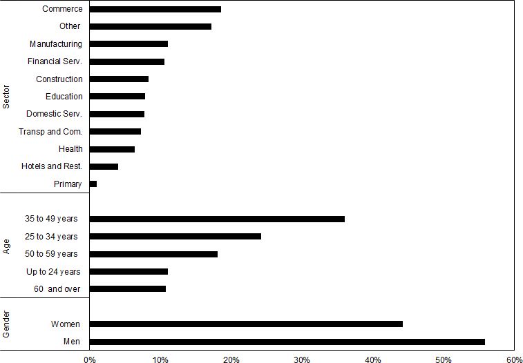
We begin by characterizing the pre-COVID-19 scenario, corresponding to the first quarter of 2020. According to the EPH, approximately 12 million people were employed during the first quarter of 2020. Figure 1 shows the distribution of workers among gender, age groups, and economic sectors. Male workers represent 56 percent of total employees, and around 78 percent of all workers were 25 to 59 years old. The most relevant economic sectors in terms of employment were commerce (19 percent), financial services (11 percent), and manufacturing (11 percent). The informality rate was, on average, 40 percent but was decreasing on the income level.

Pre-COVID-19 scenario. Distribution of workers by gender, age groups, and sectors.. Source: Authors’ own calculations based on Ministry of Labor, Employment and Social Security and INDEC. Notes: In percentage.
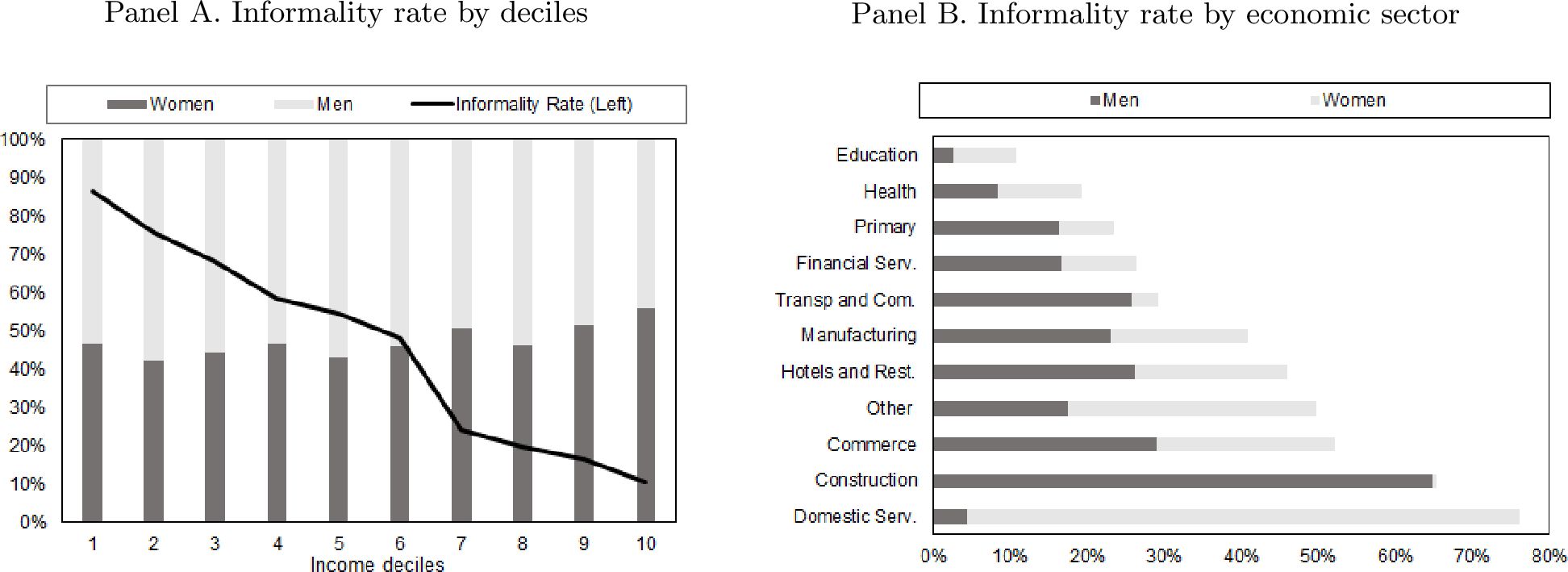
Panel A in Figure 2 indicates that for the lowest (highest) income decile, the informality rate is near 85 (10) percent. The share of woman between informal workers seems to be slightly higher as income levels increase. Informality also varies among economic sectors (see Panel B in Figure 2), with domestic services being the sector with the higher informality rate (76 percent) and with higher relative participation of woman among informal workers. Construction is another sector with high informality but is mostly made up by male workers. Education and health sectors also have a relatively low informality rate.

Pre-COVID-19 scenario. Share of informal workers by deciles, gender, and sectors.
Table 1, Column [1] presents the average per capita income for pre-COVID-19 scenario. For the first quarter of 2020, it was $19,914, slightly higher for households with a male household head (see Table A4). The richest decile shows an income approximately 22 times higher than the poorest. Table 2, Column [1] provides the same information but distinguishes between economic sectors instead of income deciles.26 The table also shows a wide heterogeneity across sectors. Highest per capita incomes can be appreciated in primary activities, financial services, and social and health services. Domestic services, construction, hotels, and restaurants are among sector with lowest incomes.
Average per capita income by deciles. Pre- and post-COVID-19 scenarios with and without policy responses.
| Pre-COVID-19 | Post-COVID-19 scenario (without policy responses) | Post-COVID-19 scenario (with policy responses) | |||||||||||
|---|---|---|---|---|---|---|---|---|---|---|---|---|---|
| 1st quarter 2020 | 1 quarter ahead | 2 quarters ahead | 3 quarters ahead | 1 quarter ahead | 2 quarters ahead | 3 quarters ahead | |||||||
| Decile | [1] | [2] | [3] | [4] | [5] | [6] | [7] | [8] | [9] | [10] | [11] | [12] | [13] |
| Level | Level | Level | Change [4] - [1] (in %) | Level | Change [6] - [2] (in %) | Level | Change [8] - [2] (in %) | Level | Change [10] - [1] (in %) | Level | Change [12] - [6] (in %) | ||
| 1 | 2841.8 | 1974.0 | 2396.1 | -15.69 | 2387.2 | 20.9 | 2842.7 | 44.0 | 3205.8 | 12.8 | 2977.3 | 24.7 | |
| 2 | 5822.4 | 4250.3 | 5004.4 | -14.05 | 4813.7 | 13.3 | 4924.5 | 15.9 | 5623.7 | -3.4 | 5272.9 | 9.5 | |
| 3 | 8189.0 | 6176.9 | 7258.7 | -11.36 | 6884.8 | 11.5 | 6762.2 | 9.5 | 7777.8 | -5.0 | 7216.8 | 4.8 | |
| 4 | 10367.5 | 7807.2 | 9200.6 | -11.26 | 8641.3 | 10.7 | 8294.3 | 6.2 | 9628.1 | -7.1 | 8882.4 | 2.8 | |
| 5 | 12978.9 | 10347.1 | 11763.7 | -9.36 | 11096.3 | 7.2 | 10769.7 | 4.1 | 12139.6 | -6.5 | 11302.5 | 1.9 | |
| 6 | 16019.6 | 12918.2 | 14818.0 | -7.50 | 13599.7 | 5.3 | 13262.0 | 2.7 | 15125.3 | -5.6 | 13778.4 | 1.3 | |
| 7 | 19789.5 | 16368.6 | 18590.6 | -6.06 | 17035.5 | 4.1 | 16628.7 | 1.6 | 18830.7 | -4.8 | 17201.9 | 1.0 | |
| 8 | 25037.3 | 21413.7 | 23702.7 | -5.33 | 21507.7 | 0.4 | 21645.3 | 1.1 | 23917.8 | -4.5 | 21648.2 | 0.7 | |
| 9 | 33516.6 | 28733.5 | 32248.0 | -3.78 | 28544.9 | -0.7 | 28899.3 | 0.6 | 32393.6 | -3.4 | 28632.5 | 0.3 | |
| 10 | 64559.5 | 54499.1 | 62174.1 | -3.69 | 53405.3 | -2.0 | 54617.7 | 0.2 | 62283.2 | -3.5 | 53458.7 | 0.1 | |
| All | 19914.0 | 16450.4 | 18717.4 | -6.01 | 16793.1 | 2.1 | 16866.1 | 2.5 | 19094.2 | -4.1 | 17038.6 | 1.5 | |
-
Source: Authors’ own calculations based on Ministry of Production and Labor and EPH-INDEC. Notes: In pesos and percentage change. Deciles of per capita income. Workers in Argentina benefit from a wage bonus, aguinaldos, that is paid twice a year in June and December. Therefore, they are registered and included in the first and third quarters of our simulations but not in the second and fourth ones. Thus, to provide an accurate comparison, the pre-COVID-19 scenario should be compared with the second-quarter-ahead scenario. This is valid for both the scenario with and without policy responses.
Average per capita income by economic sector. Pre- and post-COVID-19 scenarios with and without policy responses.
| Pre-COVID-19 | Post-COVID-19 scenario (without policy responses) | Post-COVID-19 scenario (with policy responses) | |||||||||||
|---|---|---|---|---|---|---|---|---|---|---|---|---|---|
| 1st quarter 2020 | 1 quarter ahead | 2 quarters ahead | 3 quarters ahead | 1 quarter ahead | 2 quarters ahead | 3 quarters ahead | |||||||
| Sector | [1] | [2] | [3] | [4] | [5] | [6] | [7] | [8] | [9] | [10] | [11] | [12] | [13] |
| Level | Level | Level | Change [4] - [1] (in %) | Level | Change [6] - [2] (in %) | Level | Change [8] - [2] (in %) | Level | Change [10] - [1] (in %) | Level | Change [12] - [6] (in %) | ||
| Primary activities | 35381.3 | 21090.5 | 30087.9 | -15.0 | 26230.8 | 24.4 | 21475.7 | 1.8 | 30381.8 | -14.1 | 26371.9 | 0.5 | |
| Manufacturing | 19020.6 | 15046.6 | 17550.6 | -7.7 | 15612.8 | 3.8 | 15475.1 | 2.8 | 17934.3 | -5.7 | 15805.1 | 1.2 | |
| Construction | 14493.5 | 11537.6 | 13414.3 | -7.4 | 12220.9 | 5.9 | 12143.8 | 5.3 | 13973.7 | -3.6 | 12508.1 | 2.3 | |
| Commerce | 18401.6 | 14723.3 | 17100.0 | -7.1 | 15525.3 | 5.4 | 15222.0 | 3.4 | 17555.6 | -4.6 | 15757.6 | 1.5 | |
| Hotels and rest. | 17049.4 | 12384.3 | 15147.9 | -11.2 | 13652.5 | 10.2 | 12929.2 | 4.4 | 15621.6 | -8.4 | 13863.4 | 1.5 | |
| Transp. and com. | 24533.3 | 19042.1 | 22514.4 | -8.2 | 19857.1 | 4.3 | 19379.4 | 1.8 | 22809.8 | -7.0 | 20001.7 | 0.7 | |
| Financial serv. | 28750.7 | 23060.5 | 26614.6 | -7.4 | 23550.0 | 2.1 | 23382.0 | 1.4 | 26895.2 | -6.5 | 23663.0 | 0.5 | |
| Education | 27983.4 | 23147.5 | 26406.0 | -5.6 | 22707.2 | -1.9 | 23274.8 | 0.5 | 26517.7 | -5.2 | 22749.4 | 0.2 | |
| Social-health serv. | 28959.7 | 24465.7 | 27630.8 | -4.6 | 23864.5 | -2.5 | 24641.0 | 0.7 | 27787.5 | -4.0 | 23940.1 | 0.3 | |
| Domestic serv. | 12080.5 | 9108.9 | 10891.3 | -9.8 | 9969.3 | 9.4 | 9935.1 | 9.1 | 11662.2 | -3.5 | 10285.2 | 3.2 | |
| Other serv. | 21463.2 | 17921.9 | 20225.8 | -5.8 | 18127.4 | 1.1 | 18367.1 | 2.5 | 20634.8 | -3.9 | 18318.0 | 1.1 | |
| All | 24460.2 | 19423.3 | 22737.1 | -7.0 | 19843.0 | 2.2 | 19819.1 | 2.0 | 23093.7 | -5.6 | 20004.7 | 0.8 | |
-
Source: Authors’ own calculations based on Ministry of Production and Labor and EPH-INDEC. Notes: In pesos and percentage change. Deciles of per capita income. Workers in Argentina benefit from a wage bonus, aguinaldos, that is paid twice a year in June and December. Therefore, they are registered and included in the first and third quarters of our simulations but not in the second and fourth ones. Thus, to provide an accurate comparison, the pre-COVID-19 scenario should be compared with the second-quarter-ahead scenario. This is valid for both the scenario with and without policy responses.
Table 3, Panel A, Column [1] shows that these figures on per capita income results in a Gini coefficient of 0.441. Income inequality was more pronounced among female-headed households (0.458; Panel B, Column [1]). In terms of indigence and poverty, 8.59 percent of the population was indigent, and the poverty rate was around 34.5 percent, which represents around 9.8 million people (Panel C, Column [1]). Again, the poverty incidence is higher for households with a female head (38.5 versus 31.8; Panel B, Column [1]).
Poverty, inequality indicators, and number of poor by gender. Pre- and post-COVID-19 scenarios with and without policy responses.
| Pre-COVID-19 | Post-COVID-19 scenario (without policy responses) | Post-COVID-19 scenario (with policy responses) | ||||||||||||
|---|---|---|---|---|---|---|---|---|---|---|---|---|---|---|
| 1st quarter 2020 | 1 quarter ahead | 2 quarters ahead | 3 quarters ahead | 1 quarter ahead | 2 quarters ahead | 3 quarters ahead | ||||||||
| Sector | Group | [1] | [2] | [3] | [4] | [5] | [6] | [7] | [8] | [9] | [10] | [11] | [12] | [13] |
| Level | Level | Level | Change [4] - [1] (in %) | Level | Change [6] - [2] (in %) | Level | Change [8] - [2] (in %) | Level | Change [10] - [1] (in %) | Level | Change [12] - [6] (in %) | |||
| Panel A. Indigence, poverty, and inequality indicators | ||||||||||||||
| Extreme poverty | ||||||||||||||
| FGT (0) | 8.6 | 18.0 | 12.5 | 45.3 | 13.3 | -26.3 | 15.3 | -14.8 | 10.0 | 16.6 | 11.2 | -15.3 | ||
| FGT (1) | 3.2 | 10.1 | 6.1 | 90.9 | 6.1 | -40.3 | 7.1 | -30.4 | 4.1 | 28.9 | 4.8 | -20.2 | ||
| FGT (2) | 1.9 | 7.7 | 4.3 | 123.7 | 4.2 | -46.1 | 4.5 | -42.4 | 2.5 | 31.0 | 3.3 | -20.6 | ||
| Moderate poverty | ||||||||||||||
| FGT (0) | 34.6 | 45.6 | 39.2 | 13.5 | 43.3 | -5.2 | 43.8 | -4.0 | 37.3 | 7.9 | 42.0 | -3.0 | ||
| FGT (1) | 13.6 | 22.9 | 17.7 | 29.7 | 19.0 | -16.9 | 20.2 | -11.7 | 15.5 | 13.4 | 17.5 | -7.9 | ||
| FGT (2) | 7.6 | 15.6 | 11.1 | 46.0 | 11.6 | -25.5 | 12.6 | -18.9 | 8.9 | 17.7 | 10.2 | -12.0 | ||
| Inequality | ||||||||||||||
| Gini | 0.441 | 0.465 | 0.455 | 3.1 | 0.444 | -4.7 | 0.465 | -0.1 | 0.450 | 1.9 | 0.435 | -2.0 | ||
| Theil | 0.345 | 0.382 | 0.366 | 6.0 | 0.347 | -9.1 | 0.381 | -0.2 | 0.357 | 3.5 | 0.333 | -4.0 | ||
| ATK (0) | 0.000 | 0.000 | 0.000 | 0.000 | 0.000 | 0.000 | 0.000 | |||||||
| ATK (0.5) | 0.160 | 0.181 | 0.171 | 6.9 | 0.162 | -10.4 | 0.180 | -0.4 | 0.167 | 4.2 | 0.154 | -4.7 | ||
| ATK (1) | 0.300 | 0.347 | 0.323 | 7.9 | 0.306 | -11.8 | 0.344 | -0.8 | 0.315 | 5.1 | 0.289 | -5.5 | ||
| ATK (2) | 0.546 | 0.645 | 0.596 | 9.0 | 0.562 | -12.9 | 0.625 | -3.1 | 0.582 | 6.4 | 0.525 | -6.7 | ||
| Panel B. Poverty and inequality indicators, by gender | ||||||||||||||
| Moderate poverty | ||||||||||||||
| Poverty | Head male | 31.8 | 43.3 | 36.4 | 14.3 | 41.3 | -4.6 | 41.4 | -4.5 | 34.3 | 8.0 | 40.2 | -2.9 | |
| Incidence | Head female | 38.6 | 49.0 | 43.4 | 12.5 | 46.1 | -5.9 | 47.4 | -3.4 | 41.6 | 7.9 | 44.6 | -5.9 | |
| Population | 34.6 | 45.6 | 39.2 | 13.5 | 43.3 | -5.2 | 43.8 | -4.0 | 37.3 | 7.9 | 42.0 | -4.2 | ||
| Inequality | ||||||||||||||
| Gini | Head male | 0.429 | 0.444 | 0.439 | 2.4 | 0.428 | -3.5 | 0.446 | 0.3 | 0.435 | 1.4 | 0.420 | -5.6 | |
| Head female | 0.458 | 0.496 | 0.478 | 4.2 | 0.465 | -6.2 | 0.492 | -0.9 | 0.470 | 2.5 | 0.454 | -7.6 | ||
| Population | 0.441 | 0.465 | 0.455 | 3.1 | 0.444 | -4.7 | 0.465 | -0.1 | 0.450 | 1.9 | 0.435 | -6.5 | ||
| Panel C. Number of poor | ||||||||||||||
| Head male | 5,376,778 | 7,324,550 | 6,147,894 | 771,116 | 6,986,696 | -337,854 | 6,997,154 | -327,396 | 5,804,325 | 427,547 | 6,795,035 | -191,661 | ||
| Head female | 4,489,291 | 5,698,983 | 5,045,405 | 556,114 | 5,365,024 | -333,959 | 5,505,334 | -193,649 | 4,841,836 | 352,545 | 5,181,325 | -183,699 | ||
| Population | 9,866,069 | 13,023,533 | 11,193,299 | 1,327,230 | 12,351,720 | -671,813 | 12,502,488 | -521,045 | 10,646,161 | 780,092 | 11,976,360 | -375,360 | ||
-
Source: Authors’ own calculations based on Ministry of Production and Labor and EPH-INDEC. Notes: Workers in Argentina benefit from a wage bonus, aguinaldos, that is paid twice a year in June and December. Therefore, they are registered and included in the first and third quarters of our simulations but not in the second and fourth ones. Thus, to provide an accurate comparison, the pre-COVID-19 scenario should be compared with the second-quarter-ahead scenario. This is valid for both the scenario with and without policy responses.
3.2. Post-COVID-19 scenarios without policy responses
As previously mentioned, the COVID-19 shock was the largest economic contraction that Argentina experienced after the Great Recession of 2008/2009. During the second quarter of 2020, the county experienced an output reduction of around 20 percent. Naturally, this shock had considerable effects on employment. Given that this output contraction was almost twice during the COVID-19 shock than it was in the Great Recession, we assume that employment reductions during the second quarter of 2020 were twice as those experienced during the Great Recession.27 Under this assumption, employment among formal workers was reduced—during the second quarter of 2020—by 24.2 percent and by 47 percent among informal workers (see Table A1). Drops in informal employment were higher than those in formal employment for all economic sectors. In our simulations around 2.6 million people lost their jobs between the second and the first quarter of 2020.
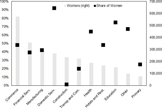
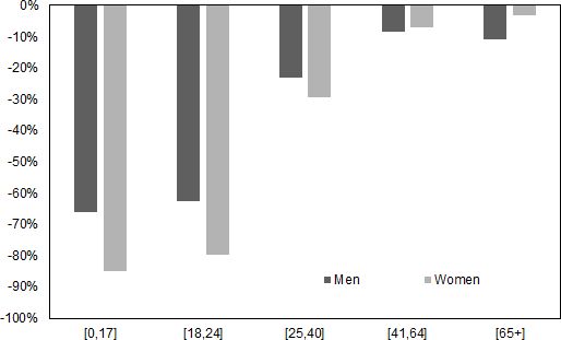
In line with Figure 1, higher absolute drops in employment were in commerce, financial services, manufacturing, domestic services, and construction. The share of women who lost their jobs varies among sectors, with domestic service being the sector in which women were more affected as 92 percent of new unemployed workers were women (Figure 3). When looking at the employment rate, the contraction was relatively higher among women than men (–23 percent versus –20.8 percent, respectively). In early working ages (18–24) the differences are large: the fall in the employment rate was 63 percent for men and 80 percent for women (Figure 4). These differences become more pronounced when considering the presence of children. For example, for the age group between 18 and 24, the contraction in employment for men with children was close to 57 percent, while for women with children it was 82 percent. In the group between 25 and 40 years old, the falls were 18 percent and 30 percent, respectively. Even conditioning on sectors, In 7 of the 11 analyzed sectors, women’s employment was more affected than that of men (see Table A3).28

Post-COVID-19 scenario. Simulation of employment loss and relative participation of woman. By sectors.. Source: Authors’ own calculations based on Ministry of Labor, Employment and Social Security and INDEC. Notes: In thousands of workers and percentage. Second quarter of 2020.

Post-COVID-19 scenario. Change on employment rate by age groups and gender.. Source: Authors’ own calculations based on Ministry of Labor, Employment and Social Security and INDEC. Notes: In percentage. Second quarter versus first quarter 2020.
In the simulated post-COVID-19 scenarios without policy responses, average per capita income decreased by about 6 percent (Table 1, Column [5]).29 However, this reduction was nonlinear along the income distribution. While the richest decile showed an income reduction of approximately 3.7 percent, the reduction among the poorest was around 15.7 percent.30 This is explained by the fact that informal workers are concentrated at the bottom of the income distribution and were the ones most affected by the crisis (they are not protected by labor regulations).31 The results for this scenario in terms of poverty and income distribution were as expected (Table 3, Panel A, Columns [4] and [5]). Indigence sharply rose up to 12.4 percent, 45.3 percent higher when comparing to pre-COVID-19 scenario. Poverty incidence rose up to 39.22 (13.5 percent higher, when comparing with the pre-COVID-19 scenario).
Interestingly, the poverty measures that consider their severity like FGT(1) and FGT(2) present larger increases. Increases in poverty incidence were similar for female-headed households (12.5 percent) and male-headed households (14.3 percent). This change in poverty represented an additional of 1.3 million people under the poverty line (Table 3, Panel C, Column [4]). According to our simulation, these “new poor” individuals are those who work in the informal sector either as wage earners or self-employed, and their dependents. These individuals belong to households with an average size of around five people and where 44 percent are children. They are mostly employed in sectors such as construction, domestic service, hotels and restaurants, and manufacturing. In terms of education, they have approximately 6 years of education, which represents 2.4 years less than the average for the total population. Income inequality also worsened substantially; the Gini coefficient for this scenario was 0.455, 3.1 percent higher than the one corresponding to the pre-COVID-19 scenario. This could be related to the fact that the lowest deciles experienced higher income reductions, relative to the highest deciles.
Continuing with the post-COVID-19 scenarios without policy responses, an interesting exercise is to compare the third quarter ahead with the first quarter ahead (i.e., a comparison with the probable worst moment of the pandemic). This provides a sense of the evolution of income and employment net of public assistance, that is, changes that can be associated with economic activity only. Table 1, Column [7] shows that household income, on average, increased by 2.1 percent, but the differential effect on income distribution remains. The income of the richest decile fell by 2 percent, while the income of the poorest decile increased by 20.9 percent. This, consistent with administrative data, may be due to a faster recovery of informal employment—which has a greater relative weight in the lower part of the income distribution—than formal employment.
Following the INDEC, the employment rate for informal (formal) wage earners increased from 6.1 (19.6) percent to 7.7 (19) percent between the second and the third quarter of 2020. This recovery of income occurs precisely in sectors that have a relatively higher percentage of informality such as domestic services, construction, and commerce (Table 2, Column [7]).32 Consistent with this evolution of income, poverty and income distribution responded as expected (Table 3, Panel A, Column [7]). Indigence was reduced by 26.3 percent, and poverty incidence fell by 5.2 percent; this change represents around 0.6 million people jumping the poverty line (Panel C, Column [6]). Income inequality also improved substantially. The Gini coefficient for the third-quarter-ahead scenario is 0.444, 4.7 percent lower than the first-quarter-ahead scenario after COVID-19 (0.465).
3.3. Post-COVID-19 scenarios with policy responses
When considering government policy responses, the post-COVID-19 scenario seems to have ameliorated. A comparison with the pre-COVID-19 scenario shows a contrast where economic activity and policy responses are, jointly, the main drivers behind changes. In this scenario (Table 1, Column [11]), average per capita income reduced by about 4.1 percent when compared to the pre-COVID-19 scenario. Thus, public assistance cushioned by around one-third what the average drop in household income would have been (–4.1 in Column [11] versus -6.0 in Column [5]). For a household at the second decile, income was reduced by 3.4 percent with policy responses, but without public assistance this reduction would have been 14.1 percent. This “cushioning” effect of public assistance occurred, albeit with decreasing intensity, in the following deciles.
Further, as expected, the policy responses do not seem to have been impacted substantially in the top 20 percent of the income distribution. And when analyzing by economic sectors, the findings are similar. It is worth noting, though, that public assistance ameliorated the scenario of some exposed (to COVID-19) activities. For example, construction workers’ incomes reduced by 3.6 percent (Table 2, Column [11]). This reduction would have been 7.4 percent without policy responses (Column [5]). Similar conclusions can be found for other sectors such as domestic services and hotels and restaurants.
Public assistance also ameliorated the scenario in terms of poverty and income distribution (Table 3, Panel A, Columns [10] and [11]). Indigence increased by 10.02 percent, 16.6 percent more when compared to the pre-COVID-19 scenario. It is worth recalling that this 10.02 would have been 12.48 in the absence of policy responses (Panel A, Columns [5]). Poverty incidence rose up to 37.31 (2.73 percentage points or 7.9 percent higher, when comparing with the pre-COVID-19 scenario), implying a reduction of 2.46 (1.92) percentage points in the indigence (poverty) rate when compared to the scenario without policy responses (Panel A, 10.02 (37.31) in Column [10] versus 12.48 (39.22) in Column [5]). This effect prevented more than 0.55 million people from falling into poverty (Panel C, Column [10]).
Policy responses were equally important in alleviating poverty in female- and male-headed households. For the former, poverty rose from 38.58 to 41.65 (Panel B, Column [1] and [10]), while it would have increased to 43.40 in the scenario without policy responses (Column [4]). This represents a cushion of 1.75 percentage points, or 4 percent (1.75/43.40). In the case of male-headed households, the cushion was 2.03 percentage points (34.34 –- 36.37), or 5.6 percent (2.03/36.37). Income inequality also ameliorated substantially. The Gini coefficient for this scenario is 0.450, pretty similar to the one corresponding to that of the pre-COVID-19 scenario (Panel A, Column [10]).
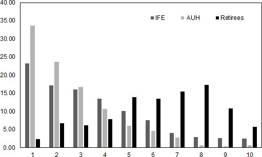
To better understand these results, it is useful to characterize the public assistance beneficiaries. In our simulations, around 10 million people received some kind of public cash transfers. We identify 4.7 million who received IFE, 3.5 million who received a bonus for AUH, and 2.7 million retirees. The share of women among these groups is 54 percent, 57 percent, and 67 percent, respectively. Figure 5 presents how these beneficiaries are distributed along the income distribution. The figure shows that AUH is the most pro-poor cash transfer, with around 84 percent of its beneficiaries at the bottom 40 percent of the income distribution. Approximately 72 percent of IFE´s beneficiaries are also at this bottom 40 percent. This is in line with previous figures on informality. Given that eligibility criteria for IFE were informal workers, unemployed workers, and low-income self-employed workers and that informal workers are in the bottom of the income distribution, logically, IFE´s beneficiaries will be concentrated there. Finally, the less pro-poor distribution is associated with retirees and pensioners; only around 23 percent are at the bottom 40 percent of the income distribution.

Distribution of public assistance beneficiaries.. Source: Authors’ own calculations based on EPH-INDEC. Notes: In percentage. By deciles of per capita income. Second quarter of 2020.
Finally, comparing the same quarters between scenarios with and without policy responses could provide additional relevant insights regarding policy effects. Note that here, policy responses will be, uniquely, the main driver behind the changes since the economic activity driver is the same in both scenarios. For this purpose, in Column [9] of each table (i.e. Tables 1 and 2), we compare the percentage change of income levels and poverty and inequality indicators at the first quarter after the pandemic with and without policy responses. In Column [13] of Tables 1 and 2 we do the same for the third quarter. The results indicate that average per capita familiar income was consistently higher, on average, in all quarters compared to what it would have been without public assistance. This holds, naturally with a different intensity, for both the lower and upper sides of the income distribution. Given that we assume that the intensity of public assistance decreases as the economy reduced its rate of contraction, this seems to be correlated with the fact that in the first quarter after the pandemic, household income was, on average, 2.5 higher compared to what it would have been without public assistance (Table 1, Column [9]). During the third quarter, this difference decreased to 1.5 percent (Column [13]). This phenomenon can also be seen when analyzing the dynamics of income by economic sectors (Columns [9] and [13]).
The gradual withdrawal of public assistance is also consistent with its lower intensity to reduce indigence and poverty and to improve the income distribution. In terms of indigence reduction, during the first quarter post-COVID-19, public assistance reduced the indigence rate by 14.8 percent (Table 3, Panel A, Column [9]). Despite the economy falling so much, and incomes slowly recovering, lower public assistance reduced indigence by 15.3 percent in the third quarter (Panel A, Column [13]). In terms of poverty, it is interesting to look at the absolute values of individuals. During the first quarter, public assistance contributed to preventing nearly a half million people from falling into poverty (521,045 in Table 3, Panel C, Column [9]). Yet, in the third quarter, and with a lower number of poor people, public assistance helped another 400,000 people avoid becoming poor (375,360 in Panel C, Column [13]).
4. Conclusions and recommendations for policy discussion
While the health effects of the COVID-19 crisis were the initial focus of the government, its socioeconomic effects and accompanying policy responses have been receiving more attention, mainly in low- and middle-income countries. In this context we analyze the impact of the COVID-19 crisis on households’ incomes, unemployment, poverty, and inequality in Argentina. For this purpose, using a standard microsimulation methodology we simulate impacts on welfare at the household level using household survey data and administrative data on employment and wages by economic sectors. The simulations also include public cash transfers (i.e., policy responses), implemented by the government to mitigate the crisis, to get a sense of how effective these policy measures were in counteracting those negative effects.
The results indicate that during the COVID-19 crisis, households would have experienced a reduction of about 6 percent on their incomes without any policy responses. This reduction was nonlinear along the income distribution, with the lowest income earners suffering the most in relative terms. This result is strongly related with relatively higher informality at the bottom of the income distribution. The greater negative effects of the pandemic in less well-off parts of the income distribution are in line with results from Bonavida and Gasparini (2020). Furthermore, the impact was not homogeneous by gender: on average, the employment rate fell more among women than men (–23 percent versus –20.8 percent when comparing the second and first quarters of 2020). In early working ages (18–24), the differences are very significant: the fall in the employment rate was 63 percent for men and 80 percent for women. These differences become more pronounced when considering the presence of children. For example, for the 18–24 age group, the contraction in employment for men with children was close to 57 percent, while it was 82 percent for women with children. In the 25–40 age group, the contractions were 18 percent and 30 percent, respectively. Moreover, even when conditioning on sectors, in 7 of the 11 analyzed sectors, women’s employment was more affected than that of men. These findings are consistent with ILO (2020) and are associated with the overlap of work responsibilities and care responsibilities (housework, childcare and eldercare), which have intensified during the pandemic, especially for households with children (OECD, 2020; WEF, 2021). In addition, we find that the policy response cushioned by around one-third what the average drop in household income would have been. This prevented major increases in poverty and inequality. A key aspect of the satisfactory policy response was that public assistance was targeted at informal workers and at less well-off households with children. This policy response’s large offsetting effect is in line with previous findings such as Lustig et al. (2020).
Our simulations face two main limitations. First, there are limited data available on how the pandemic is affecting economic activity in real time. At the moment of writing this paper, only the household survey corresponding to the first quarter of 2020 was available in Argentina. Also, information on how employment in the different sectors was being affected has been published with lags. Second, we have lack knowledge on how to predict how the pandemic will evolve. Argentina, like the rest of the countries in the world, are going through the pandemic without certainty about when or how it will yield.
In the transition toward the end of the pandemic, policy discussions should include short- and medium-term policies. For short-term policies, policymakers and academics should focus on how to accurately target public assistance. An important lesson from the Argentine case is that as most of poorest households are employed in the informal sector, relief measures—such as those applied in this paper—considering informality becomes crucial. Thus, it becomes very important to discuss policies aimed at reducing labor informality as labor market policies play an important role in the formalization of employment. Given that most informal workers have low qualifications and work in jobs that are difficult to identify for public policies, an integrated policy approach is necessary, which includes economic, social, and labor policies (Bertranou et al., 2013). Along these lines, it is also important to address how to adapt people to the transformation of the workplace in the post-COVID-19 era since the crisis may allow wider adoptions of teleworking practices.
Also crucial in policy discussions is accurately identifying those who really need public assistance. All information about citizens, contained in the administrative records of the different divisions of the public sector, must be used. Invest in resources and modern technologies to obtain a good handling of this information should also be considered to have it available at the right times. In turn, it is important to make efforts to get this information as updated as possible. All this aims to minimize the typical errors of inclusion and exclusion that arise when targeting social policies. An adequate use of the administrative records of the Argentine social security, through its different contributory and non-contributory programs, despite its limitations, is a key aspect since it already covers most of the population (Giuliano et al., 2020).
Footnotes
1.
Additionally, with the objective of containing the decline in productive activity, the government created the Assistance Program for Emergency to Work and Production (ATP in Spanish). Through this program, the national government helps firms—that applied to the program—by paying 50 percent of wages to employees.
2.
According to Argentina’s Ministry of Economy, during 2020, current transfers registered a year-on-year increase of $153 billion pesos, of which $114 billion were received by the private sector. Payments for the Emergency Family Income (IFE) and the ATP amounted to $11 billion (2 GDP points), and family allowances increased by $22 billion by virtue of the increases granted through decrees no. 163/20, no. 495/20, and no. 692/20 and the mobility applied during 2019.
3.
These are the periods between June and March 2020 (first-quarter-ahead scenario), July and September 2020 (second-quarter-ahead scenario), and October and December 2020 (third-quarter-ahead scenario).
4.
Women usually bear most of the childcare and housework; see Angelov et al. (2016) and Bertrand (2020).
5.
For the San Francisco Bay area, Martin et al. (2020) also find that government benefits decrease the amplitude of the crisis.
6.
As remarked by Janssens et al. (2021), most of the evidence is from developed countries. See, for example, Coibion et al. (2020), Forsythe et al. (2020), and Montenovo et al. (2020).
7.
Similarly, and for the United States, Montenovo et al. (2020) show that job loss is larger in occupations that cannot be performed remotely.
8.
Unfortunately, the EPH, which is the main household survey in Argentina, does not cover rural areas. This is a strong data limitation that prevents us from understanding the distributional effects of COVID-19 in rural areas. Beyond the possibility that urban areas have been the epicenter of the pandemic, we believe that this paper is an appropriate attempt to approximate the effects of COVID-19 in Argentina at the beginning of the pandemic given the data availability.
9.
We do not impute the rental value of owner-occupied housing.
10.
The impacts can take one or more of the following forms: (a) a decline in quantity of work, either hours (intensive margin) or employment (extensive margin); (b) a decline in wages, which is unlikely for salaried workers in the short run but may occur over time due to furloughs or wage cuts by some employers to avoid layoffs; (c) a decline in the income of self-employed workers due to the reduction of economic activity (sales, production) in micro and small enterprises due to the fall in demand and disruptions in supply of inputs or due to mobility restrictions, particularly for migrants engaged in seasonal agriculture.
11.
We do not consider the effect of price changes given that in Argentina home production is negligible, and so net producer/consumer models are not relevant for this country. In addition, we also do not consider the remittances given that they are not a relevant component of households’ income. In 2019, remittances only accounted for 0.11 of GDP.
12.
This is the latest wave available at the time of writing this paper.
13.
See here for the official methodology on poverty estimation in Argentina.
14.
To calculate poverty and indigence (i.e., extreme poverty) following INDEC, we modify the gipc by dividing the total income of the household by the number of equivalent adult members of the household (that is, a man between 30 and 60 years based on calorie needs) instead of just the number of members. We use the traditional FGT poverty indicators (Foster et al., 1984), considering poverty lines (and extreme poverty) that vary according to the geographical location of the household (i.e., region) due to the variation in the price level. Specifically, these regions are: Gran Buenos Aires, Noroeste Argentino, Noreste Argentino, Cuyo, Pampa, Patagonia.
15.
Note that the quarters correspond to the second, third, and fourth quarters of 2020.
16.
See here. These data provide quarterly information on the number of formal and informal workers by economic sector.
17.
Given that at the time of this simulation there are no data on changes in employment.
18.
For example, during the Great Recession, output experienced the highest contraction during the second quarter of 2009, of 11.3 percent. Formal (informal) employment in primary sector fell, on average, by 33.1 (47.3) percent. During the second quarter of 2020, output reduced by 19 percent. Thus, we assume that the primary sector reduction on formal employment was 62.9 (89.8). See Table A1.
19.
The first group includes age, age squared, gender, marital status, and indicator variables for educational levels. Household-level variables include the logarithm of the household’s per capita income and the number of household members. See Table A2. Although some of these variables may be endogenous, we do not think it is a major concern since the aim of this model is prediction.
20.
An implicit assumption that we are making is that there are no formal-informal transitions and all of those selected to lose their job go to unemployment/inactivity. Note that allowing for formal-informal transitions would lead to smaller effects on poverty. Consequently, we are estimating an upper-bound of that effect. Although it can be considered as a limitation of the microsimulation, our intention is to capture the maximum effect on the poverty rate (i.e., the most damaging scenario for the Argentine economy).
21.
We exclude business owners, non-salaried family workers, and public sector employees when simulating employment losses. Public sector employment is very stable in Argentina and there were no systematic layoffs during this period. See Table A1.
22.
We collapse labor income to zero for those individuals who are selected to lose their job, and we impute the percentage change in wages for those who remain employed. Note that the income that collapses to zero is labor income, which is the focus of our simulation. This assumption could be very restrictive if individuals lose their jobs, lose their income, and use savings or sell assets during unemployment. These income components—other than labor—are not modeled or considered in equation 1. If these types of effects exist, the income effects captured in this paper could be considered bound effects (e.g., lower bound effects if the income collapse is, partially or completely, offset through assets sales or spending saving).
23.
According to the INDEC, 36.1 percent was the annual rate of inflation for 2020.
24.
Our simulations only indirectly consider the ATP program. Since this program was granted to companies to pay salaries and avoid dismissals, the wage and employment figures we use for the simulation implicitly contemplate it.
25.
In other words, we follow the benefit incidence analysis, one of the most widely used methodologies for policy response simulation (van de Walle, 1995; Bourguignon et al., 2003; Gasparini et al., 2014; Lustig, 2017).
26.
See Table A5 for a more detailed sectorial effect when considering the household head’s gender.
27.
Output reductions during the third and fourth quarters of 2020 represent 1.1 and 0.9 times the decline associated with the Great Recession, respectively. Therefore, the simulated scenarios for these periods assume that the falls in employment were 1.1 and 0.9 times the falls in employment experienced during the Great Recession, respectively.
28.
These results should be taken with caution since we are not testing the significance of the gender differences.
29.
Remember that given the inclusion of aguinaldos, an accurate comparison with the pre-COVID-19 scenario (first quarter of 2020) must be made with the second quarter ahead of the post-COVID-19 scenario.
30.
For the case of Janssens et al. (2021) find a similar reduction of around one-third in the poorest household incomes. Martin et al. (2020) perform a simulation for the San Francisco Bay area and also document that the lowest income earners suffer the most in relative terms.
31.
32.
See Table A1.
Appendix
Simulated policy response to mitigate the effects of the COVID-19 crisis
At the beginning of the COVID-19 crisis, on March 23, 2020, through decree 310/2020, the National Social Security Administration (ANSES) created the IFE benefit aimed at the most vulnerable sectors of the population. The IFE consists of an exceptional non-contributory monetary benefit, intended to compensate the loss or serious decrease in income of people affected by the health emergency scenario (declared by decree no. 260/2020). To mitigate the increase in poverty and indigence, this measure was aimed at households composed of informal workers, unemployed workers, and low-income self-employed workers. The latter are those with an monthly average gross income of less than $17,394 (around US$220); that is, those sectors of the population with the highest degree of vulnerability in socioeconomic terms.
The amount of the IFE was $10,000 (around US$120, which represents 60 percent of the minimum wage) and can be collected by a member of the household who is under conditions of exclusion or job insecurity and is facing socioeconomic vulnerability. The IFE presents two exclusive definitions regarding the delimitation of the beneficiary population. On the one hand, it provides assistance to workers affected by precarious job placement (low-income self-employed workers, domestic workers, informal employees, and unemployed workers). On the other hand, the program limits this coverage to the employment and economic situation of the household to which the beneficiary belongs, in the sense that all its members must meet the conditions to access the IFE and only one of them may receive the benefit. The IFE was compatible with the receipt of other social programs like the AUH or the AUE.
Simultaneously with the IFE, a bonus of up to $3,000 (around US$40) was granted to more than 4.6 million retirees and pensioners who received a single pension until reaching $18,892 (around US$240). In addition, the amount of the AUH and the AUE was doubled, benefiting more than 4.3 million children and adolescents who received a supplementary income of $3,103.
Supplementary Tables
Employment and wage variations.
| Employment variations | ||||||
|---|---|---|---|---|---|---|
| Sector | 1q ahead | 2q ahead | 3q ahead | |||
| Formal | Informal | Formal | Informal | Formal | Informal | |
| Primary | -0.63 | -0.90 | -0.36 | -0.52 | -0.30 | -0.43 |
| Manufacturing | -0.18 | -0.33 | -0.10 | -0.19 | -0.08 | -0.16 |
| Construction | -0.17 | -0.27 | -0.10 | -0.15 | -0.08 | -0.13 |
| Commerce | -0.12 | -0.44 | -0.07 | -0.25 | -0.06 | -0.21 |
| Hotels and rest. | -0.31 | -0.45 | -0.18 | -0.26 | -0.15 | -0.21 |
| Transp. and com. | -0.19 | -0.44 | -0.11 | -0.25 | -0.09 | -0.21 |
| Financial serv. | -0.25 | -0.44 | -0.14 | -0.26 | -0.12 | -0.21 |
| Education | -0.28 | -0.72 | -0.16 | -0.42 | -0.13 | -0.34 |
| Health | -0.17 | -0.58 | -0.10 | -0.33 | -0.08 | -0.27 |
| Domestic serv. | -0.24 | -0.29 | -0.14 | -0.17 | -0.11 | -0.14 |
| Other | -0.12 | -0.33 | -0.07 | -0.19 | -0.06 | -0.15 |
| Average | -0.24 | -0.47 | -0.14 | -0.27 | -0.11 | -0.22 |
| Wage variations | ||||||
| Formal | Informal | Formal | Informal | Formal | Informal | |
| -0.0034 | 0.02 | 0.05 | 0.13 | 0.16 | 0.25 | |
-
Source: Authors’ own calculations based on Ministry of Production and Labor and EPH-INDEC. Notes: We assume zero variations on public employment. For wage variations, we use the same criteria than for the rest of employees (INDEC). These are, for each quarter, 1,95 percent, 7.19 percent, and 15.22 percent, respectively.
Logistic regression on the probability of being employed: Formal and informal workers.
| Pr (employed=1) | ||
|---|---|---|
| Formal | Informal | |
| Gender (male==1) | 1.307*** | 1.275*** |
| (0.344) | (0.317) | |
| Age | 0.212*** | 0.0964*** |
| (0.0157) | (0.0135) | |
| Age2 | -0.00198*** | -0.000818*** |
| (0.000184) | (0.000165) | |
| Incomplete primary | -0.265 | -0.891 |
| (0.976) | (0.804) | |
| Complete primary | 0.496 | -0.561 |
| (0.925) | (0.782) | |
| Incomplete secondary | 0.334 | -0.773 |
| (0.918) | (0.776) | |
| Complete secondary | 0.637 | -0.86 |
| (0.915) | (0.774) | |
| Incomplete tertiary | 0.406 | -0.897 |
| (0.917) | (0.776) | |
| Complete tertiary | 1.053 | -1.14 |
| (0.904) | (0.763) | |
| Head of HH | 0.845*** | 0.484*** |
| (0.121) | (0.104) | |
| # of children | 0.237** | 0.127 |
| (0.111) | (0.0968) | |
| Marriage status | 0.627*** | 0.368*** |
| (0.0796) | (0.0674) | |
| # HH members | 0.156*** | 0.0783*** |
| (0.0231) | (0.0177) | |
| HH per capita income (log) | 2.013*** | 0.552*** |
| (0.062) | (0.0439) | |
| Observations | 11,656 | 8,478 |
| R2 | 0.3613 | 0.0645 |
-
Source: Authors’ own estimates based on the Permanent Household Survey (EPH). Notes: Robust standard errors are in parentheses. Statistical significance *** p < 0.01, ** p < 0.05, * p < 0.1. Interaction terms and intercept are included but not reported for briefness.
Employment by gender. Pre-COVID-19 (1st quarter of 2020) versus Post-COVID-19 (2nd quarter of 2020). Number of employed people and percentage change.
| 1st quarter 2020 | 2nd quarter 2020 | Change | |||||||
|---|---|---|---|---|---|---|---|---|---|
| Level | Level | % | |||||||
| Male | Female | All | Male | Female | All | Male | Female | All | |
| Primary | 91,750 | 29,883 | 121,633 | 34,636 | 10,945 | 45,581 | -62.2 | -63.4 | -62.5 |
| Manufacturing | 874,726 | 451,827 | 1,326,553 | 708,487 | 332,908 | 1,041,395 | -19.0 | -26.3 | -21.5 |
| Construction | 1,044,273 | 22,001 | 1,066,274 | 810,563 | 19,909 | 830,472 | -22.4 | -9.5 | -22.1 |
| Commerce | 1,311,071 | 883,783 | 2,194,854 | 1,012,360 | 608,865 | 1,621,225 | -22.8 | -31.1 | -26.1 |
| Hotels and rest. | 278,457 | 183,943 | 462,400 | 191,980 | 104,309 | 296,289 | -31.1 | -43.3 | -35.9 |
| Transp. and com. | 778,999 | 135,834 | 914,833 | 598,012 | 91,637 | 689,649 | -23.2 | -32.5 | -24.6 |
| Financial serv. | 783,739 | 528,898 | 1,312,637 | 566,354 | 389,737 | 956,091 | -27.7 | -26.3 | -27.2 |
| Education | 239,797 | 735,108 | 974,905 | 201,445 | 623,182 | 824,627 | -16.0 | -15.2 | -15.4 |
| Health | 1,033,530 | 1,123,807 | 2,157,337 | 965,203 | 1,004,377 | 1,969,580 | -6.6 | -10.6 | -8.7 |
| Domestic serv. | 47,380 | 942,717 | 990,097 | 24,948 | 697,099 | 722,047 | -47.3 | -26.1 | -27.1 |
| Other | 246,806 | 276,809 | 523,615 | 214,327 | 211,890 | 426,217 | -13.2 | -23.5 | -18.6 |
| Total | 6,730,528 | 5,314,610 | 12,045,138 | 5,328,315 | 4,094,858 | 9,423,173 | -20.8 | -23.0 | -21.8 |
-
Source: Authors’ own estimates based on Permanent Household Survey (EPH). Notes: The table includes all types of employment (public, private, and self-employment).
Average per capita income by deciles and by gender. Pre- and post-COVID-19 scenarios with and without policy responses. In pesos and percentage change.
| Pre-COVID-19 | Post-COVID-19 scenario (without policy responses) | Post-COVID-19 scenario (with policy responses) | ||||||||||||
|---|---|---|---|---|---|---|---|---|---|---|---|---|---|---|
| 1st quarter 2020 | 1 quarter ahead | 2 quarters ahead | 3 quarters ahead | 1 quarter ahead | 2 quarters ahead | 3 quarters ahead | ||||||||
| Decil | Group | [1] | [2] | [3] | [4] | [5] | [6] | [7] | [8] | [9] | [10] | [11] | [12] | [13] |
| Level | Level | Level | Change[4] - [1](in %) | Level | Change[6] - [2](in %) | Level | Change [8] - [2](in %) | Level | Change [10] - [1](in %) | Level | Change [12] - [6] (in %) | |||
| 1 | Head male | 2876.8 | 2019.1 | 2386.4 | -17.05 | 2382.7 | 18.0 | 2812.6 | 39.3 | 3114.0 | 8.2 | 2856.4 | 19.9 | |
| Head female | 2810.4 | 1933.5 | 2404.7 | -14.43 | 2391.3 | 23.7 | 2869.8 | 48.4 | 3288.3 | 17.0 | 3085.9 | 29.1 | ||
| Decile | 2841.8 | 1974.0 | 2396.1 | -15.69 | 2387.2 | 20.9 | 2842.7 | 44.0 | 3205.8 | 12.8 | 2977.3 | 24.7 | ||
| 2 | Head male | 5881.1 | 4534.6 | 5227.2 | -11.12 | 5008.1 | 10.4 | 5173.8 | 14.1 | 5795.6 | -1.5 | 5413.6 | 8.1 | |
| Head female | 5754.5 | 3920.8 | 4746.2 | -17.52 | 4588.4 | 17.0 | 4635.6 | 18.2 | 5424.5 | -5.7 | 5109.7 | 11.4 | ||
| Decile | 5822.4 | 4250.3 | 5004.4 | -14.05 | 4813.7 | 13.3 | 4924.5 | 15.9 | 5623.7 | -3.4 | 5272.9 | 9.5 | ||
| 3 | Head male | 8223.8 | 6429.1 | 7382.5 | -10.23 | 6966.7 | 8.4 | 7001.6 | 8.9 | 7889.2 | -4.1 | 7301.9 | 4.8 | |
| Head female | 8138.5 | 5810.2 | 7078.7 | -13.02 | 6765.8 | 16.4 | 6414.1 | 10.4 | 7615.7 | -6.4 | 7093.1 | 4.8 | ||
| Decile | 8189.0 | 6176.9 | 7258.7 | -11.36 | 6884.8 | 11.5 | 6762.2 | 9.5 | 7777.8 | -5.0 | 7216.8 | 4.8 | ||
| 4 | Head male | 10352.4 | 7943.7 | 9356.1 | -9.62 | 8676.8 | 9.2 | 8400.7 | 5.8 | 9757.7 | -5.7 | 8876.9 | 2.3 | |
| Head female | 10389.5 | 7609.1 | 8974.6 | -13.62 | 8589.7 | 12.9 | 8139.7 | 7.0 | 9439.9 | -9.1 | 8890.4 | 3.5 | ||
| Decile | 10367.5 | 7807.2 | 9200.6 | -11.26 | 8641.3 | 10.7 | 8294.3 | 6.2 | 9628.1 | -7.1 | 8882.4 | 2.8 | ||
| 5 | Head male | 12904.4 | 10491.4 | 11875.5 | -7.97 | 11122.0 | 6.0 | 10852.8 | 3.4 | 12204.3 | -5.4 | 11323.5 | 1.8 | |
| Head female | 13082.1 | 10147.3 | 11608.8 | -11.26 | 11060.8 | 9.0 | 10654.5 | 5.0 | 12050.0 | -7.9 | 11273.4 | 1.9 | ||
| Decile | 12978.9 | 10347.1 | 11763.7 | -9.36 | 11096.3 | 7.2 | 10769.7 | 4.1 | 12139.6 | -6.5 | 11302.5 | 1.9 | ||
| 6 | Head male | 16017.4 | 13231.7 | 14856.3 | -7.25 | 13547.2 | 2.4 | 13519.3 | 2.2 | 15123.6 | -5.6 | 13710.4 | 1.2 | |
| Head female | 16023.9 | 12326.6 | 14745.6 | -7.98 | 13698.8 | 11.1 | 12776.4 | 3.6 | 15128.6 | -5.6 | 13906.7 | 1.5 | ||
| Decile | 16019.6 | 12918.2 | 14818.0 | -7.50 | 13599.7 | 5.3 | 13262.0 | 2.7 | 15125.3 | -5.6 | 13778.4 | 1.3 | ||
| 7 | Head male | 19768.0 | 16373.9 | 18662.9 | -5.59 | 17113.0 | 4.5 | 16612.0 | 1.5 | 18883.1 | -4.5 | 17261.5 | 0.9 | |
| Head female | 19819.5 | 16361.2 | 18490.0 | -6.71 | 16927.5 | 3.5 | 16651.9 | 1.8 | 18757.7 | -5.4 | 17118.9 | 1.1 | ||
| Decile | 19789.5 | 16368.6 | 18590.6 | -6.06 | 17035.5 | 4.1 | 16628.7 | 1.6 | 18830.7 | -4.8 | 17201.9 | 1.0 | ||
| 8 | Head male | 24920.4 | 21226.2 | 23533.0 | -5.57 | 21187.1 | -0.2 | 21430.0 | 1.0 | 23721.8 | -4.8 | 21320.8 | 0.6 | |
| Head female | 25243.5 | 21744.7 | 24002.2 | -4.92 | 22073.2 | 1.5 | 22025.2 | 1.3 | 24263.6 | -3.9 | 22225.9 | 0.7 | ||
| Decile | 25037.3 | 21413.7 | 23702.7 | -5.33 | 21507.7 | 0.4 | 21645.3 | 1.1 | 23917.8 | -4.5 | 21648.2 | 0.7 | ||
| 9 | Head male | 33505.8 | 28632.5 | 32187.2 | -3.94 | 28267.5 | -1.3 | 28791.9 | 0.6 | 32330.1 | -3.5 | 28354.1 | 0.3 | |
| Head female | 33536.6 | 28922.2 | 32361.5 | -3.50 | 29063.2 | 0.5 | 29100.1 | 0.6 | 32512.2 | -3.1 | 29152.7 | 0.3 | ||
| Decile | 33516.6 | 28733.5 | 32248.0 | -3.78 | 28544.9 | -0.7 | 28899.3 | 0.6 | 32393.6 | -3.4 | 28632.5 | 0.3 | ||
| 10 | Head male | 64176.4 | 53944.6 | 61847.3 | -3.63 | 52654.1 | -2.4 | 54050.2 | 0.2 | 61947.0 | -3.5 | 52708.0 | 0.1 | |
| Head female | 65193.7 | 55416.9 | 62714.9 | -3.80 | 54648.5 | -1.4 | 55557.0 | 0.3 | 62839.6 | -3.6 | 54701.1 | 0.1 | ||
| Decile | 64559.5 | 54499.1 | 62174.1 | -3.69 | 53405.3 | -2.0 | 54617.7 | 0.2 | 62283.2 | -3.5 | 53458.7 | 0.1 | ||
| All | Head male | 20717.0 | 17218.3 | 19557.8 | -5.60 | 17406.4 | 1.1 | 17583.7 | 2.1 | 19888.1 | -4.0 | 17616.4 | 1.2 | |
| Head female | 18746.6 | 15334.1 | 17495.6 | -6.67 | 15901.6 | 3.7 | 15823.0 | 3.2 | 17940.1 | -4.3 | 16198.6 | 1.9 | ||
| Population | 19914.0 | 16450.4 | 18717.4 | -6.01 | 16793.1 | 2.1 | 16866.1 | 2.5 | 19094.2 | -4.1 | 17038.6 | 1.5 | ||
-
Source: Authors’ own calculations based on Ministry of Production and Labor and EPH-INDEC. Notes: Workers in Argentina benefit from a wage bonus, aguinaldos, that is paid twice a year in June and December. Therefore, they are registered and included in the first and third quarters of our simulations but not in the second and fourth ones. Thus, to provide an accurate comparison, the pre-COVID-19 scenario should be compared with the second-quarter-ahead scenario. This is valid for both the scenario with and without policy responses.
Average per capita income by economic sector and by gender. Pre- and post-COVID-19 scenarios with and without policy responses. In pesos and percentage change.
| Pre-COVID-19 | Post-COVID-19 scenario (without policy responses) | Post-COVID-19 scenario (with policy responses) | ||||||||||||
|---|---|---|---|---|---|---|---|---|---|---|---|---|---|---|
| 1st quarter 2020 | 1 quarter ahead | 2 quarters ahead | 3 quarters ahead | 1 quarter ahead | 2 quarters ahead | 3 quarters ahead | ||||||||
| Sector | Group | [1] | [2] | [3] | [4] | [5] | [6] | [7] | [8] | [9] | [10] | [11] | [12] | [13] |
| Level | Level | Level | Change [4] - [1] (in %) | Level | Change [6] - [2] (in %) | Level | Change [8] - [2] (in %) | Level | Change [10] - [1] (in %) | Level | Change [12] - [6] (in %) | |||
| Primary act. | Head male | 36813.8 | 22837.4 | 32161.1 | -12.6 | 27830.7 | 21.9 | 23202.8 | 1.6 | 32424.3 | -11.9 | 27945.6 | 0.4 | |
| Head female | 30860.1 | 15576.9 | 23544.3 | -23.7 | 21181.2 | 36.0 | 16024.4 | 2.9 | 23934.9 | -22.4 | 21405.0 | 1.1 | ||
| Sector | 35381.3 | 21090.5 | 30087.9 | -15.0 | 26230.8 | 24.4 | 21475.7 | 1.8 | 30381.8 | -14.1 | 26371.9 | 0.5 | ||
| Manufac- turing | Head male | 19989.8 | 16026.3 | 18621.2 | -6.8 | 16331.7 | 1.9 | 16396.8 | 2.3 | 18954.0 | -5.2 | 16485.8 | 0.9 | |
| Head female | 17260.7 | 13267.5 | 15606.6 | -9.6 | 14307.4 | 7.8 | 13801.5 | 4.0 | 16082.7 | -6.8 | 14568.9 | 1.8 | ||
| Sector | 19020.6 | 15046.6 | 17550.6 | -7.7 | 15612.8 | 3.8 | 15475.1 | 2.8 | 17934.3 | -5.7 | 15805.1 | 1.2 | ||
| Constru- ction | Head male | 14908.3 | 12140.8 | 13967.8 | -6.3 | 12659.0 | 4.3 | 12779.0 | 5.3 | 14558.4 | -2.3 | 12928.4 | 2.1 | |
| Head female | 13641.8 | 10299.1 | 12277.8 | -10.0 | 11321.5 | 9.9 | 10839.4 | 5.2 | 12773.2 | -6.4 | 11645.0 | 2.9 | ||
| Sector | 14493.5 | 11537.6 | 13414.3 | -7.4 | 12220.9 | 5.9 | 12143.8 | 5.3 | 13973.7 | -3.6 | 12508.1 | 2.3 | ||
| Commerce | Head male | 18750.6 | 15335.0 | 17579.7 | -6.2 | 15853.3 | 3.4 | 15799.7 | 3.0 | 18006.8 | -4.0 | 16066.3 | 1.3 | |
| Head female | 17827.3 | 13716.8 | 16310.7 | -8.5 | 14985.7 | 9.3 | 14271.4 | 4.0 | 16813.1 | -5.7 | 15249.8 | 1.8 | ||
| Sector | 18401.6 | 14723.3 | 17100.0 | -7.1 | 15525.3 | 5.4 | 15222.0 | 3.4 | 17555.6 | -4.6 | 15757.6 | 1.5 | ||
| Hotels and rest. | Head male | 17423.5 | 13116.4 | 15739.9 | -9.7 | 14196.0 | 8.2 | 13640.7 | 4.0 | 16204.1 | -7.0 | 14368.0 | 1.2 | |
| Head female | 16560.2 | 11427.0 | 14373.7 | -13.2 | 12941.8 | 13.3 | 11998.8 | 5.0 | 14859.8 | -10.3 | 13203.5 | 2.0 | ||
| Sector | 17049.4 | 12384.3 | 15147.9 | -11.2 | 13652.5 | 10.2 | 12929.2 | 4.4 | 15621.6 | -8.4 | 13863.4 | 1.5 | ||
| Tran. and com. | Head male | 24247.9 | 19141.4 | 22432.7 | -7.5 | 19678.4 | 2.8 | 19477.1 | 1.8 | 22731.1 | -6.3 | 19824.2 | 0.7 | |
| Head female | 25173.4 | 18819.4 | 22697.5 | -9.8 | 20257.9 | 7.6 | 19160.1 | 1.8 | 22986.2 | -8.7 | 20399.6 | 0.7 | ||
| Sector | 24533.3 | 19042.1 | 22514.4 | -8.2 | 19857.1 | 4.3 | 19379.4 | 1.8 | 22809.8 | -7.0 | 20001.7 | 0.7 | ||
| Financial serv. | Head male | 29727.0 | 24441.8 | 27713.6 | -6.8 | 24574.5 | 0.5 | 24728.0 | 1.2 | 27967.8 | -5.9 | 24683.9 | 0.4 | |
| Head female | 26969.8 | 20540.5 | 24609.8 | -8.8 | 21681.1 | 5.6 | 20926.5 | 1.9 | 24938.6 | -7.5 | 21800.6 | 0.6 | ||
| Sector | 28750.7 | 23060.5 | 26614.6 | -7.4 | 23550.0 | 2.1 | 23382.0 | 1.4 | 26895.2 | -6.5 | 23663.0 | 0.5 | ||
| Education | Head male | 28563.8 | 23565.4 | 26985.3 | -5.5 | 22982.5 | -2.5 | 23658.5 | 0.4 | 27069.8 | -5.2 | 23015.4 | 0.1 | |
| Head female | 27261.2 | 22627.4 | 25685.2 | -5.8 | 22364.7 | -1.2 | 22797.2 | 0.8 | 25830.7 | -5.2 | 22418.4 | 0.2 | ||
| Sector | 27983.4 | 23147.5 | 26406.0 | -5.6 | 22707.2 | -1.9 | 23274.8 | 0.5 | 26517.7 | -5.2 | 22749.4 | 0.2 | ||
| Soc. and health | Head male | 30351.3 | 25821.1 | 29034.2 | -4.3 | 25062.0 | -2.9 | 25963.8 | 0.6 | 29162.2 | -3.9 | 25120.4 | 0.2 | |
| Head female | 26952.0 | 22510.3 | 25606.0 | -5.0 | 22136.8 | -1.7 | 22732.7 | 1.0 | 25804.1 | -4.3 | 22237.4 | 0.5 | ||
| Sector | 28959.7 | 24465.7 | 27630.8 | -4.6 | 23864.5 | -2.5 | 24641.0 | 0.7 | 27787.5 | -4.0 | 23940.1 | 0.3 | ||
| Domestic serv. | Head male | 12683.2 | 9882.2 | 11586.0 | -8.7 | 10526.5 | 6.5 | 10427.7 | 5.5 | 12094.6 | -4.6 | 10771.9 | 2.3 | |
| Head female | 11652.9 | 8560.4 | 10398.5 | -10.8 | 9574.0 | 11.8 | 9585.7 | 12.0 | 11355.6 | -2.6 | 9939.9 | 3.8 | ||
| Sector | 12080.5 | 9108.9 | 10891.3 | -9.8 | 9969.3 | 9.4 | 9935.1 | 9.1 | 11662.2 | -3.5 | 10285.2 | 3.2 | ||
| Other serv. | Head male | 21020.8 | 17336.8 | 19808.2 | -5.8 | 17438.2 | 0.6 | 17710.4 | 2.2 | 20149.1 | -4.1 | 17577.5 | 0.8 | |
| Head female | 22221.4 | 18924.4 | 20941.3 | -5.8 | 19308.4 | 2.0 | 19492.4 | 3.0 | 21467.2 | -3.4 | 19586.9 | 1.4 | ||
| Sector | 21463.2 | 17921.9 | 20225.8 | -5.8 | 18127.4 | 1.1 | 18367.1 | 2.5 | 20634.8 | -3.9 | 18318.0 | 1.1 | ||
| All | Head male | 24977.5 | 20058.8 | 23392.5 | -6.3 | 20294.4 | 1.2 | 20405.7 | 1.7 | 23705.5 | -5.1 | 20434.2 | 0.7 | |
| Head female | 23659.2 | 18439.3 | 21722.3 | -8.2 | 19144.0 | 3.8 | 18910.9 | 2.6 | 22146.5 | -6.4 | 19339.6 | 1.0 | ||
| All Sectors | 24460.2 | 19423.3 | 22737.1 | -7.0 | 19843.0 | 2.2 | 19819.1 | 2.0 | 23093.7 | -5.6 | 20004.7 | 0.8 | ||
-
Source: Authors’ own calculations based on Ministry of Production and Labor and EPH-INDEC. Notes: Workers in Argentina benefit from a wage bonus, aguinaldos, that is paid twice a year in June and December. Therefore, they are registered and included in the first and third quarters of our simulations but not in the second and fourth ones. Thus, to provide an accurate comparison, the pre-COVID-19 scenario should be compared with the second-quarter-ahead scenario. This is valid for the scenario with and without the policy response.
References
-
1
Parenthood and the Gender Gap in PayJournal of Labor Economics 34:545–579.https://doi.org/10.1086/684851
-
2
COVID19 on Welfare: A Microsimulation Approach. Unpublished Technical NotePartnership for Economic Policy (PEP).
-
3
Gender in the Twenty-First CenturyAEA Papers and Proceedings 110:1–24.https://doi.org/10.1257/pandp.20201126
-
4
Dónde, Cómo y Por Qué Se Redujo La Informalidad Laboral En Argentina Durante El Período 2003-2012Documentos de trabajo, N° 1. Oficina de País de la OIT para la Argentina.
-
5
El Impacto Asimétrico de la Cuarentena. CEDLAS, Working Papers 0261CEDLAS, Universidad Nacional de La Plata.
-
6
The Impact of Economic Policies on Poverty and Income Distribution: Evaluation Techniques and ToolsWorld Bank Publications, no. 15090. The World Bank.
-
7
Too little but not too late: nowcasting poverty and cash transfers’ incidence during COVID-19’s crisisWorld Development 140:105227.https://doi.org/10.1016/j.worlddev.2020.105227
-
8
The Cost of the Covid-19 Crisis: Lockdowns, Macroeconomic Expectations, and Consumer Spending. NBER Working Papers 27141National Bureau of Economic Research, Inc.
-
9
Labor demand in the time of COVID-19: Evidence from vacancy postings and UI claimsJournal of Public Economics 189:104238.https://doi.org/10.1016/j.jpubeco.2020.104238
- 10
-
11
CEDLAS, Working Papers 0171Pobreza y Desigualdad en America Latina: Conceptos, Herramientas y Aplicaciones, CEDLAS, Working Papers 0171, CEDLAS, Universidad Nacional de La Plata.
-
12
Distributional effects of reducing energy subsidies: Evidence from recent policy reform in ArgentinaEnergy Economics 92:C.
- 13
-
14
The short-term economic effects of COVID-19 on low-income households in rural Kenya: An analysis using weekly financial household dataWorld Development 138:C.https://doi.org/10.1016/j.worlddev.2020.105280
-
15
Policy Research Working Paper Series 9503Impacts of COVID-19 on Household Welfare in Tunisia, Policy Research Working Paper Series 9503, The World Bank, 10.1596/1813-9450-9503.
-
16
El impacto del sistema tributario y el gasto social en la distribución del ingreso y la pobreza en América Latina. Una aplicación del marco metodológico del proyecto Compromiso con la Equidad (CEQ)El Trimestre Económico pp. 493–568.
-
17
The Impact of COVID-19 Lockdowns and Expanded Social Assistance on Inequality, Poverty and Mobility in Argentina, Brazil, Colombia and MexicoECINEQ, Society for the Study of Economic Inequality.
-
18
Socio-Economic Impacts of COVID-19 on Household Consumption and PovertyEconomics of Disasters and Climate Change 4:453–479.https://doi.org/10.1007/s41885-020-00070-3
-
19
Determinants of Disparities in Covid-19 Job LossesNational Bureau of Economic Research, Inc.
-
20
https://www.oecd.org/coronavirus/policy-responses/women-at-the-core-of-the-fight-against-covid-19-crisis-553a8269/https://www.oecd.org/coronavirus/policy-responses/women-at-the-core-of-the-fight-against-covid-19-crisis-553a8269/.
-
21
Policy Research Working Paper Series 1476Public spending and the poor: what we know, what we need to know, Policy Research Working Paper Series 1476, The World Bank.
- 22
-
23
Poverty and Distributional Impacts of COVID-19: Potential Channels of Impact and Mitigating PoliciesThe World Bank.
Article and author information
Author details
Julian Martinez-Correa

Funding
No specific funding for this article is reported.
Acknowledgements
This work was carried out with financial and scientific support from the Partnership for Economic Policy (PEP), with funding from the Government of Canada through the International Development Research Centre (IDRC). We thank three anonymous reviewers for suggestions, clarification requests, and useful comments. We also thank Edgar Cooke and the attendees at our presentation during PEP´s Annual Conference for useful comments and suggestions. Antonn Park provided an excellent edition of the paper. The usual disclaimer applies.
Publication history
- Version of Record published: December 31, 2022 (version 1)
Copyright
© 2022, Martinez-Correa et al.
This article is distributed under the terms of the Creative Commons Attribution License, which permits unrestricted use and redistribution provided that the original author and source are credited.