The ‘German Job Miracle’ and Its Impact on Income Inequality: A Decomposition Study

Cite this article as: J. Mühlhan; 2023; The ‘German Job Miracle’ and Its Impact on Income Inequality: A Decomposition Study; International Journal of Microsimulation; 16(1); 28-64. doi: 10.34196/ijm.00274

Article
Figures and data
Jump to

Abstract

In the last 15 years before the COVID-19 crisis, Germany has experienced a strong and continuous increase in employment - the ‘German job miracle’. During this period, income inequality, which had previously increased sharply, remained relatively stable. This paper analyzes the impact of employment changes on disposable income inequality between 2004 and 2015 and gives an answer to the question why inequality remained constant despite the dramatic increase in employment. It is the first study to examine the effect of changing labor supply patterns due to changes in policies, wages and preferences, as well as the role that labor market constraints have played for inequality of disposable income. It finds that inequality would have increased further due to a transforming population structure, but increasing employment and policy changes almost completely offset this development. The results show that employment growth due to the reduction of labor market constraints has been more important in slowing down the increase in inequality than changes in labor supply.

1. Introduction

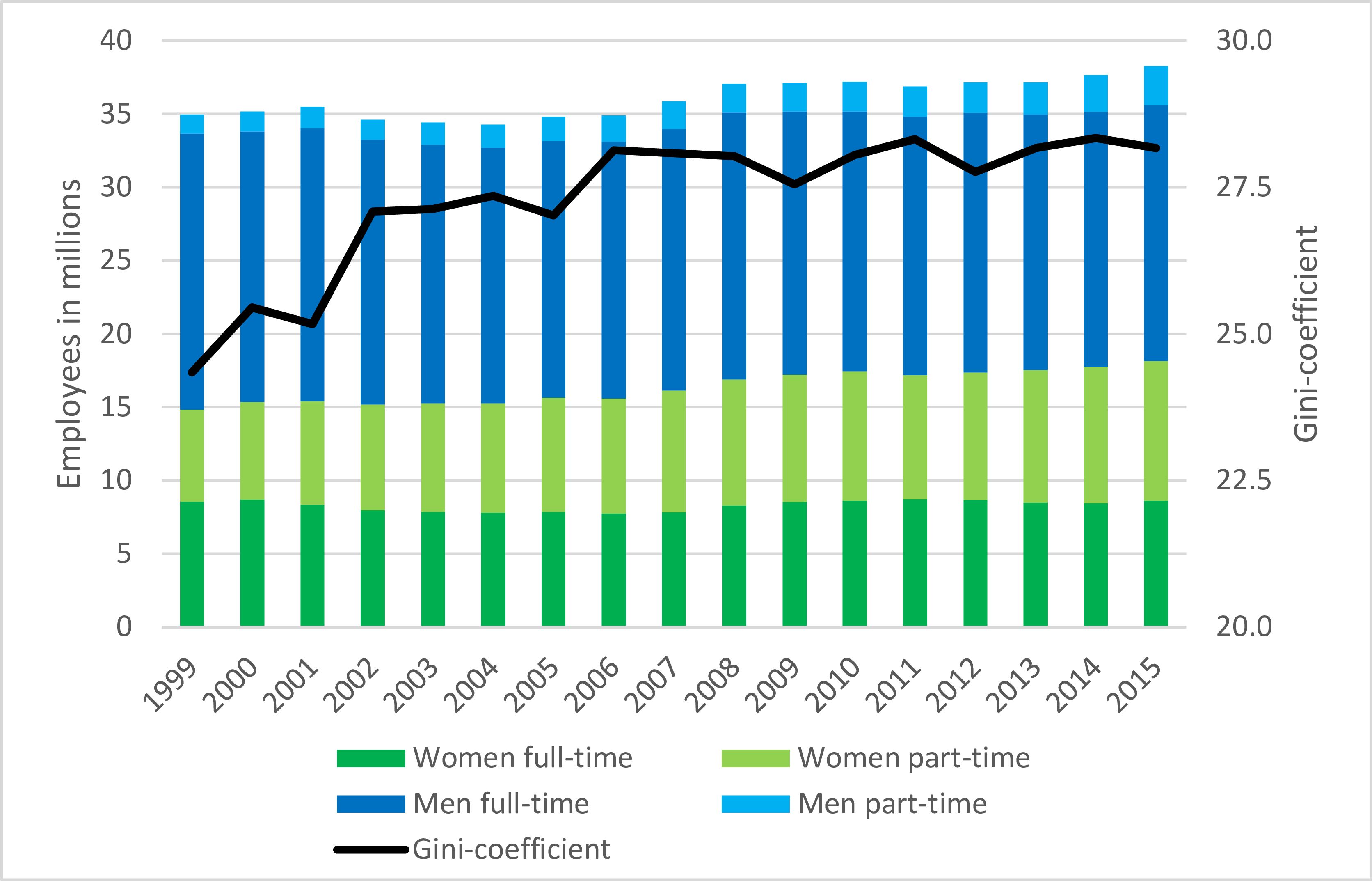
Income inequality in Germany stayed relatively stable at a low level compared to other industrialized countries and in particular the Anglo-Saxon countries until the end of the last century OECD (2008); (2011). From 1999 onward, however, there was a brief phase characterized by a sharp rise in income inequality that lasted until 2005. Between 2002 and 2005, this sharp rise in inequality was accompanied by a decline in the number of people employed. Since 2005, inequality of disposable income remained relatively stable in Germany (Peichl et al., 2018) as well as in most EU countries (Eurofound, 2017). But while other European countries experienced a long lasting and dramatical increase in unemployment rates during the global financial crisis and the European debt crisis, Germany has seen a substantial rise in employment: the ‘German job miracle’. The number of employees subject to social insurance contributions increased by more than four million between 2005 and 2015 and continued to increase until March 2020, the start of the COVID-19 crisis (Bundesagentur für Arbeit, 2019). Figure 1 shows the development of employment and inequality in Germany between 1999 and 2015 based on the German Socio-economic Panel (SOEP). It can be seen that the increase in employment is almost entirely due to the increase in part-time employment of women, which rose from 6.3 million in 1999 to 9.5 million in 2015. Increasing part-time work among men is offset by a simultaneous decline in full-time employment.

Figure 1

Download asset Open asset

Trends in inequality and employment in Germany. Note: Inequality of equivalized disposable household income. Employment numbers includes the full population and self-employment.Source: SOEP v32.1; author’s own presentation.

Since income from employment is by far the most important income source for private households in Germany (Statistisches Bundesamt, 2021), it is reasonable to assume that the German job miracle had a noticeable impact on income distribution. If the increase in employment is predominantly due to previously unemployed people from the bottom of the income distribution, this impressive increase in employees should strengthen smaller incomes in particular and reduce disposable income inequality (Eurofound, 2017; Bargain et al., 2017). This paper examines the questions whether rising employment has reduced inequality of disposable income in Germany between 2004 and 2015 and and if so, why inequality did not then decline overall. Between 2004 and 2015 Germany has seen a number of substantial social, political and economic changes that may have affected employment and the distribution of income: the revision of the welfare system completed in 2005 as well as multiple smaller adjustments in the tax and benefit system; the global financial crisis which was followed by the European debt crisis and an economic recession; an increase in wage inequality; changes in the population structure, not only due to migration. To evaluate the impact of different changes on disposable income, a static policy and wage effect as well as four different employment effects are identified: (1) labor market constraints, (2) changes in working preferences of individuals, (3) labor supply adjustments to changes in the tax and benefit system, and (4) changes in the wage structure.

The distribution of disposable income measures the actual financial inequalities between households and is therefore the relevant indicator for social policy. However, the distribution of disposable income results from the interplay of various influencing factors such as labor and other income, household composition, and the tax and transfer system. This study identifies partial changes in income inequality by generating counterfactual distributions using microsimulation techniques. A detailed depiction of the tax and benefit system allows for the analysis of employment changes not only in terms of market income but also in terms of disposable household income. Literature analysing causes of changes in disposable income inequality is surprisingly small (Biewen and Sturm, 2022) . The applied decomposition strategy builds upon a model by Bargain and Callan (2010), which quantifies the effect of tax and benefit policy on the income distribution and follows the suggestion of Bargain (2012) to additionally account for behavioral responses. Jessen (2019) extends this framework to include the introduction of wage changes. Herault and Kalb (2020) consider preference changes. This is the first decomposition that uses a double hurdle model (Bargain et al., 2010) instead of an unrestricted labor supply model to estimate the impact of behavioral responses. It provides an estimator for employment instead of supply changes by accounting for involuntary unemployment and allows to differentiate between demand and supply side induced employment changes as well as different causes of changing labor supply. Comparable to O’Donoghue (2021), this analysis measures the partial effects at the full set of possible permutations and evaluates the effect heterogeneity. It shows that the results are sensitive to the chosen decomposition order.

The ‘German job miracle’ is the subject of numerous research projects and has attracted considerable attention from policymakers in Germany and beyond, raising the question of whether the German trend could and should be emulated. However, there is no clear consensus in the literature about the causes for the increasing employment rates and the role played by the landmark Hartz reforms (Burda and Seele, 2020).

Previous decomposition studies analyze the role of employment changes and other factors for inequality in Germany, but findings differ across analytical strategies and investigated periods. Biewen and Sturm (2022) analyze the effect of employment changes on net income inequality in Germany between 2005 and 2016 by predicting employment probabilities before and after the employment boom and calculating counterfactual distributions. They find that employment changes led to income growth across all parts of the distribution, with the lower part benefiting most. This equalizing effect of employment is attenuated by other factors, mainly changes in household as well as individual characteristics and the dampening effect of the tax and benefit system. For the period between 2005 and 2011, Biewen et al. (2019) find employment gains all over the income distribution and therefore no remarkable decrease of equivalized net income inequality. Using unconditional quantile regressions, Haupt and Nollmann (2014) find that employment has been the main driver of increasing inequality of disposable income between 1999 and 2005, while demographic changes reduced poverty between 1990 and 2000. Biewen and Juhasz (2012) also assign the inequality increase between 1999 and 2006 to employment outcomes, and do not find a relevant influence of changes in the household structure. Using the same approach, combining reweighting and microsimulation techniques, Biewen et al. (2019) do also find no significant effect of population changes for 2005 to 2011. The increase in gross wage inequality is no longer reflected in disposable household inequality. Both studies find that policy has reduced inequality slightly between 1999 and 2011, while Bargain et al. (2017) detect no policy effect on inequality, but a small poverty reduction between 2008 and 2013 using static microsimulation. Using static microsimulation with behavioral adjustments, Jessen (2019) finds an inequality reducing static effect of tax and benefit as well as payment structure changes on disposable inequality for 2002 to 2011, partly compensated by behavioral responses, while population changes are the main driver of increasing inequality. Peichl et al. (2012) also argue that changes in the population structure contributed to increasing inequality in pre- and post-tax income between 1991 and 2007.

This analysis shows that employment changes, together with policy changes, played an important role in slowing down the increase of disposable income inequality since 2004. However, increasing employment does not necessarily lead to homogeneous changes of inequality. While the reduction of labor market restrictions leads to a strong employment growth and reduces inequality of disposable household income, the effects of labor supply changes on inequality between 2004 and 2015 differ by cause. Adjustments in labor supply due to policies and wage changes offset each other. Preference changes lead to a strong increase in female employment but a slight increase in inequality, as predominantly women from the upper part of the income distribution enter employment. Changes in the payment structure results in increasing gross wage inequality, but due to the redistribution within households and the tax and benefit system this is not reflected in disposable household income. Without policy changes and the reduction of involuntary unemployment, the rise in inequality would have continued between 2004 and 2015 due to changes in the population structure and non-labor income. Population trends have strong inequality-increasing effects between 2004 and 2015. Potential causes include the aging population, educational expansion, declining household sizes in particular a strong increase in single households, and increasing numbers of single parents.

The paper is structured as follows. Section 2 explains the applied decomposition approach and introduces the utilized microsimulation model of the IAB (IAB-MSM) and the SOEP data. Section 3 introduces the partial effects and shows which changes caused the employment boom. Section 4 presents the simulation results of pre-tax labor income inequality and disposable income inequality and analyzes differences between decomposition paths. Section 5 concludes.

2. Empirical strategy

2.1. Data and microsimulation model

The analysis uses data from the SOEP, a representative yearly household survey for Germany.¹ The SOEP yields information on household structure and socio-demographic characteristics of each household member, information on labor market participation, actual and desired working hours as well as income from different sources of each household member.

To calculate the income distribution in the counterfactual scenarios, the disposable income of each household for each scenario is generated using the microsimulation model of the IAB (IAB-MSM). A detailed depiction of the German tax-benefit system for the periods under investigation allows the IAB-MSM to simulate disposable income for each household of the respective population, given the respective gross income according to hourly wage rates and working hours of all household members. Deductions from gross wage income, i.e. income tax and social security contributions, and means-tested benefits are simulated using the tax and benefit functions of the IAB-MSM. For the tax-benefit simulation, the statutory regulations are implemented in the IAB-MSM as far as possible, whereby information on socio-demographic and regional variables, the income of individuals and households, and current and past working hours provided in the SOEP are used. A detailed description of the calculation of a household’s needs and income in the IAB-MSM is provided in Bruckmeier and Wiemers (2011). Other income, e.g., capital income and pensions, is taken from survey information (see Table A2 in Appendix A).

Due to high demands on the data, a household selection for the microsimulation analysis is necessary.² In a first step, households are dropped in which either the head of the household or their partner could not be interviewed or the address register data indicate for some households that a partner has not been interviewed in that respective year. Approximately 80% of all households are surveyed in the first quarter of a year. Therefore, income data collected retrospectively in the following year is exploited. This analysis employs data of the SOEP waves 2004 and 2005 as well as 2015 and 2016. Therefore, in a second step, households that have not been observed for two consecutive years are excluded from the income simulation but kept in the data for inequality analysis. Additionally, missing information on certain household and personal variables requires further adjustments on the data: Missing values in variables on wages, hours worked, income from renting, etc. are imputed as long as they cannot be deduced satisfactorily from other variables. If an indirect determination of important missing values is not possible, households are excluded from the simulation sample. In total 6.2% (2004) and 12.2% (2015) needs to be dropped and another 16.5% (2004) respective 21.6% (2015) can not be exploited for income simulation but considered in the inequality analysis.

The model accounts for dropped households by adjusting the households weights so that the selected sample is still representative for all private households in Germany. This is done by grouping the data using all combinations of certain discrete household variables (e.g. type of family, sex, region, formal skill, age group, number of children) and then multiplying the original household weights with the inverse of the group specific rates of exclusion.

To account for behavioral adjustments after policy changes or income changes, the IAB-MSM applies a discrete choice labor supply model (van Soest, 1995).³ Policy changes affect households’ budget constraints and employment behavior. The structural model allows to simulate the distributional effects of those labor supply adjustments. Information on desired working hours allows to estimate a double hurdle model of labor supply along the lines of Bargain et al. (2010). In order to account for involuntary unemployment, the double hurdle approach supplements the discrete choice model by a binary model restriction probability.

Following the assumption of Bargain and Callan (2010) that the error terms of the preference and restriction model are independent, both models can be estimated separately.⁴ Three different labor states are now possible for a single individual. Voluntary non-participation (NP), involuntary unemployment (UE) and employment (EMP). Equations (1) to (3) show the respective probabilities for singles.⁵

P^{N P} = P r (d = 0) = \frac{\exp (U_{0})}{\sum_{j = 0}^{J} \exp (U_{j})}

P^{U E} = P r (d §gt; 0, r = 1) = ϕ (β X) \sum_{k = 1}^{J} \frac{\exp (U_{k})}{\sum_{j = 0}^{J} \exp (U_{j})}

P^{E M P} = P r (d §gt; 0, r = 0) = (1 - ϕ (β X)) \sum_{k = 1}^{J} \frac{\exp (U_{k})}{\sum_{j = 0}^{J} \exp (U_{j})} .

The variable $d$ describes the desired working hours and variable $r$ indicates if an individual is restricted or not. The term $\phi\left(\beta X\right)$ represents the estimated individual probability of involuntary unemployment. The term $\frac{\exp\left(U_{0}\right)}{\sum_{j=0}^{J}\exp\left(U_{j}\right)}$ gives the estimated probability for the 0-hours category and $\sum_{k=1}^{J}\frac{\exp\left(U_{k}\right)}{\sum_{j=0}^{J}\exp\left(U_{j} \right)}$ gives the probability over all positive working hour categories.

The restriction model is estimated separately for women and men, while the preference model is estimated separately for different household types: single women, single men, single parents, semiflexible couples and flexible couples. In semiflexible couples, one partner is assumed not to be available for the labor market. Individuals younger than 20 or older than 64, people in education or training, self-employed and receivers of old-age pension are assumed to be inflexible.

2.2. Decomposition approach

This study aims to decompose the total difference in inequality measures between 2004 and 2015 by generating counterfactual distributions that “lie between” the observed income distribution of both years. The period between 2004 and 2015 is characterized by a strong increase in employment while inequality remained constant. This period is particularly interesting as the labor market reforms are taking effect and employment is rising continuously despite the global financial and European debt crises. Immigration to Germany is rising but moderate, so the results are not affected by the high level of immigration in the wake of the humanitarian crisis since 2015.

The applied method builds on the approach of Bargain and Callan (2010) using behavioral microsimulation to identify the effect of tax and benefit policy on the distribution of disposable income between a base period and a final period. Utilizing a structural labor supply model allows to additionally account for indirect policy effects by simulating the effects of behavioral responses due to changes in the budget constraint of households (Bargain, 2012). To evaluate the effect of wage structures on disposable income, this paper follows an approach of Bourguignon et al. (2008) and Jessen (2019). Furthermore, the behavioral microsimulation framework enables to obtain indirect wage effects due to labor supply adjustments following changes in the pricing of labor. Contrary to previous decomposition studies with indirect effects, this analysis employs a double hurdle model accounting for involuntary unemployment when estimating labor supply responses Bargain et al. (2010). Individual labor market restrictions and working preferences enter the distribution of working hours separately. This paper exploits this in order to differentiate between the impact of changes in preferences and restrictions.

The measures

I [τ_{0}^{p} (y^{00}), {P^{N P}, P^{U E}, P^{E M P}}_{0000}] a n d I [τ_{1}^{p} (y^{11}), {P^{N P}, P^{U E}, P^{E M P}}_{1111}]

describe inequality of disposable income in the base period (2004, indexed with “0”) and in the final period (2015, indexed with “1”), respectively. Thus, the total difference in inequality between the final and base period is given by

Δ = I [τ_{1}^{ρ} (y^{11}), {P^{N P}, P^{U E}, P^{E M P}}_{1111}] - I [τ_{0}^{ρ} (y^{00}), {P^{N P}, P^{U E}, P^{E M P}}_{0000}] .

The first argument of the inequality measure $I\left[\cdot\right]$ is the tax and benefit function $\tau^{l}_{k}\left(y^{mn}\right)$ , which applies the policy regime of period $k\in\{0,1\}$ to turn pre-tax labor and nonlabor income $y^{mn}$ (calculated using the population from period $m\in\{0,1\}$ and wages from period $n\in\{0,1\}$ ) into disposable income. The index $l\in\{\rho,\alpha\rho\}$ means that the set of monetary policy parameters $\rho$ (e.g., tax-brackets thresholds and maximum benefit levels) corresponding to the policy regime d_k are either used as given or are uprated according to the factor $\alpha§gt;1$ .

The second argument of the inequality measure $I\left[\cdot\right]$ is the set of choice probabilities from equations 1 - 3, $\{P^{NP},P^{UE},P^{EMP}\}_{opqr}$ , where indices $o,p,q,r\in\{0,1\}$ mean that the choice probabilities are calculated assuming the policy regime of period $o$ , wages of period $p$ , preferences as estimated for period $q$ , and labor market restrictions of period $r$ . For brevity, $\{P^{NP},P^{UE},P^{EMP}\}_{opqr}$ will be referred as $\{P\}_{opqr}$ hereafter.

The total difference $\Delta$ in inequality measure $I$ between base and final period is decomposed into a static policy and static wage effect, the effects of corresponding labor supply adjustment due to policy (indirect policy effect) and wage changes (indirect wage effect), the effect of changes in labor supply preferences and labor market restrictions and a residual population effect:

\begin{array}{ll} Δ & = I [τ_{1}^{ρ} (y^{11}), {P}_{1111}] - I [τ_{0}^{α ρ} (y^{11}), {P}_{1111}] (p o l i c y e f f e c t) \\ + I [τ_{0}^{α ρ} (y^{11}), {P}_{1111}] - I [τ_{0}^{α ρ} (α y^{10}), {P}_{1111}] (w a g e e f f e c t) \\ + I [τ_{0}^{α ρ} (α y^{10}), {P}_{1111}] - I [τ_{0}^{α ρ} (α y^{10}), {P}_{0111}] (i n d i r e c t p o l i c y e f f e c t) \\ + I [τ_{0}^{α ρ} (α y^{10}), {P}_{0111}] - I [τ_{0}^{α ρ} (α y^{10}), {P}_{0011}] (i n d i r e c t w a g e e f f e c t) \\ + I [τ_{0}^{α ρ} (α y^{10}), {P}_{0011}] - I [τ_{0}^{α ρ} (α y^{10}), {P}_{0001}] (p r e f e r e n c e e f f e c t) \\ + I [τ_{0}^{α ρ} (α y^{10}), {P}_{0001}] - I [τ_{0}^{α ρ} (α y^{10}), {P}_{0000}] (r e s t r i c t i o n e f f e c t) \\ + I [τ_{0}^{α ρ} (α y^{10}), {P}_{0000}] - I [τ_{0}^{α ρ} (α y^{00}), {P}_{0000}] (p o p u l a t i o n e f f e c t) \\ + I [τ_{0}^{α ρ} (α y^{00}), {P}_{0000}] - I [τ_{0}^{ρ} (y^{00}), {P}_{0000}] (i n c o m e g r o w t h) . \end{array}

Monetary parameters of the tax-benefit system are uprated with the parameter $\alpha$ when applying the base period tax-benefit system to the income of final period population. The same applies to the nominal income when applying the final period tax-benefit system to the base period population. Uprating ensures that the policy effect is not affected by price inflation. Bargain et al. (2015) this study uses uprating according to consumer price inflation.⁶ Adjustments of monetary parameters of the tax-benefit system by the same factor do not affect the decomposition of disposable income in linearly homogeneous tax and transfer systems (Bargain and Callan, 2010). Although the German tax and benefit system do partly not fulfill this condition (Bargain et al., 2017), the empirical findings show that the income growth effect is small for most inequality measures.⁷

The static policy effect describes differences in disposable income between the base and final periods due to changes in the income tax and social benefit system. Applying the tax-benefit system of two different years on the identical population using the tax and benefit calculator of the IAB-MSM reveals the proportion of the total difference in disposable income that is attributable to policy changes between both points in time.⁸ The policy effect comprises effects of changed tax and benefit rules as well as effects of changes in monetary parameters. Changes in the parameters deviating from the uprating parameter $\alpha$ , including constant parameters, are, however, considered policy measures. This is of particular relevance, as there was no uprating policy embedded in the German tax legislation until 2016.

The static wage effect describes distributional changes due to changes in hourly gross wages between 2004 and 2015. Following Jessen (2019), this analysis uses an Oaxaca-Blinder inspired approach to measure the distributional effect of wage changes on disposable income (Blinder, 1973; Oaxaca, 1973). A wage regression is estimated for the 2004 and 2015 populations. This analysis utilizes the Heckman-type wage regression included in the IAB-MSM accounting for selection bias Heckman (1979).⁹ Using the other period’s estimation results allows to predict counterfactual wages. In order to retain the full distribution of wages and to account for differences in the unexplained variance of wages between both periods, a random term is drawn from the distribution of residuals of the respective year and added to the deterministic part of the wage. Comparing the counterfactual with the observed distribution yields the effect of changes in the payment structure. This reflects the wage distribution if the population of one period received wages according to the wage distribution of the other period. This approach ensures that the estimated conditional wage effect includes only differences in the payment structure of a given workforce and does not cover changes in the composition of the workforce. Differences in wages due to differences between both populations – the endowment effect – are not part of the wage effect, but included in the population effect.

The decomposition strategy distinguishes further four different drivers of employment changes: labor supply adjustments due to changes in the tax and benefit system, labor supply adjustments due to hourly wage changes, changes in labor supply preferences and changes in involuntary unemployment due to labor market restrictions.

The indirect policy and wage effects describe income changes due to behavioral adjustments to policy and wage changes. The indirect policy effect comprises changes in the income distribution due to employment changes as a consequence of changes in the tax and benefit system, since policy changes affect households budget constraints and households may adjust their labor supply. Like policy changes, also changes in the hourly wages can affect the budget constraint of a household and may cause behavioral adjustments of the labor force. Both indirect employment changes are calculated by simulating the working hour distribution under the policy and wage of both period using the double hurdle model. Running the simulation on a given population for the different working hour distribution gives the indirect policy and wage effects.

The preference and restriction effect captures employment and income changes due to differences in labor supply preferences and involuntary unemployment probabilities between the base and final periods. Probabilities for different working hour categories are estimated using equations 1 - 3 for both periods.

The preference effect on employment and the distribution of income is simulated by estimating the preference towards consumption and leisure for base and final period population.¹⁰ In the next step the preferred working hour distribution for a given population under the same policy and wage is calculated by applying the preferences of 2004 and 2015. The differences in the simulated income distribution after running the tax and benefit model for both working hour distributions gives the preference effect. The procedure is the same for determining the restriction effects, but the restriction effect comprises differences in employment due to changes in individual unemployment probabilities $\phi$ estimated in the restriction part of the double hurdle model.¹¹

Further changes in inequality due to differences in the population of 2004 and 2015 are captured by the population effect. The population effect is calculated by actually changing the underlying SOEP sample. The effect describes the difference in inequality between 2004 and 2015 if both populations faced the same tax-benefit policies, wage structures, and labor market constraints and made their labor supply decisions based on the same preferences. This effect is not negligible, since it captures all differences in the characteristics of individuals and households that are not explained by the previous effects. Important population changes with a potentially relevant impact on inequality include differences in household and family types, population aging and educational expansion.

Equation 5 shows only one possible decomposition of the total effect into the eight different partial effects. However, the estimated results for each effect may depend on the underlying population. The literature on tax progressivity discusses this issue in more detail (see for example Dardanoni and Lambert (2002) or Lambert and Thoresen (2009)). O’Donoghue (2021) shows that the results of the decomposition might be very sensitive to the chosen decomposition order. Since there is no justification for a particular order and to avoid biased results by analyzing only a subset of possible permutations, this study analyzes all possible permutations of the decomposition and evaluates each effect on all different counterfactual distributions.¹² The full set of decompositions allows to identify effect heterogeneity and possible interactions between the underlying population and the different effects. The Shorrocks-Shapley value of each effect is measured by the arithmetic mean values over all decompositions (Shapley, 1953; Shorrocks, 2013). Inequality is measured via the Gini coefficient, the Atkinson index with inequality aversion parameter $\epsilon=0.5$ , and quantile ratios.

3. Simulated partial effects

3.1. Policy changes

In 2005, a general reform of the German social benefit system took place. The so-called “Hartz IV” reform was the last of a bundle of labor market reforms. While “Hartz I” and “Hartz II” expanded non-standard employment and “Hartz III” restructured the Federal Employment Agency, “Hartz IV” overhauled the transfer system. The reform aimed to activate unemployed to participate in the labor market by a variety of activating measures, following the principle of promoting and demanding (“fördern und fordern”), like training programs and sanctions.

The income-tested and non-means-tested Unemployment Benefit (UB) for the short-term unemployed remained in force after the reform, but was adjusted in terms of the maximum duration of benefit receipt and the qualifying period. In contrast, the system for long-term unemployed was generally restructured: Before 2005, two different kinds of transfers where available for employable long-term unemployed in addition to UB. Unemployment Assistance (UA) paid 53% (57% if a child lived in the household) of previous labor income and the Social Assistance (SA) guaranteed the minimum subsistence level. After the reform, the Unemployment Benefit II (UB II) replaced the UA and SA for employable individuals and their families. Social assistance continues to be in force as basic security benefit for those who are unable to work due to their age or full reduction in earning capacity.

The reform has mixed effects on households, depending on their prior income and earnings situation. Households that received relatively high UA before the reform due to a previously high income and receive UB II after the reform are among the losers of the reform. Approximately 60 % of the former UA receiving household are worse off after the reform. Because of the stricter deduction rules, employed benefit recipients are usually among the losers of the reform. However, formerly SA receiving households due to low or no UA eligibility predominantly benefit from the reform. These households are mostly among the lowest income households (Arntz et al., 2007; Becker and Hauser, 2006; Blos and Rudolph, 2005; Schulte, 2004).

The reform was perceived by many as unfair, as previous employment was no longer a determining factor for the level of long-term benefits. However, overall government spending for social benefits has increased (Biewen and Juhasz, 2012) and households in the first two income deciles have benefited financially (Arntz et al., 2007).¹³ In the following years after the Hartz reforms only minor corrections were made to the transfer system.

Contrary to the transfer system, the period between 2004 and 2015 has not seen a comprehensive tax reform, but a number of small changes to certain tax parameters. In 2005, the last step of a decrease of the top marginal tax rate was carried out. From 2002 to 2005, the rate decreased gradually from 49% to 42%, the last step in 2005 lowered it from 45% to 42%. Also the initial marginal tax rate of 19.9% was decreased gradually since 2002. In the period under investigation it has been lowered from 16% in 2004 to 15% in 2005 to finally 14% in 2009. In 2007, the so-called “rich tax” was introduced. Gross taxable incomes exceeding € 250,000 a year are taxed since then by 45%. The thresholds of the tax brackets have not been adjusted with price inflation. While the basic tax allowance was raised regularly from € 7,664 in 2004 to € 8,472 in 2015, the tax brackets slightly moved by € 400 in 2009 and by additional € 330 in 2010.

The full social security contribution rate, including contributions by employee and employer, decreased from 41.9% in 2004 to 39.55% in 2015. The upper income threshold, the individual monthly gross income above which no contributions are due, was uprated annually corresponding to wage inflation from monthly incomes of € 3,488 in 2004 to € 4,125 in 2015 for health and long-term care insurance, from € 5,200 to € 6,050 for pensions and employment insurance in West Germany and from € 4,400 to € 5,200 in East Germany. The upper bound of marginal employment income (so-called “mini-jobs”) was increased from € 400 to € 450 in 2013. Earnings below this threshold are not subject to social security contributions by the employee.

While the UB and SA parameters are uprated regularly according to income changes at the lower end of the income distribution, there was no periodic uprating policy adjusting the tax brackets according to price inflation in Germany until 2016. Therefore, households move to higher tax brackets due to nominal wage increases, even though their real income has not increased. The consequence is a creeping tax increase due to price and income inflation. Between 2004 and 2015, the lower bound of tax brackets has shifted to the right by € 730. This corresponds to an increase by 5.7 percent of the lower bound of the first progressive zone in the tax tariff and a raise of 1.4 percent of the lower bound of the linear zone while prices inflated by 19.9 percent during this period. Immervoll (2005) and Heer and Süssmuth (2013) show that the absence of an inflation adjustment may have a crucial impact on individual tax burdens, even with low inflation. Dorn et al. (2017) show that between 2011 and 2018 bracket creep in Germany reduced tax progressivity and led to an expansion of the total tax ratio. Immervoll (2005) shows that the overall increase in tax revenues dominates the bracket creep, leading to a slight decrease of disposable household income inequality. Table A3 in the Appendix presents the most important policy parameter for 2004 and 2015 as well as the uprated monetary parameter for 2004 to compare which monetary parameter have kept pace with price inflation.

3.2. Wage changes

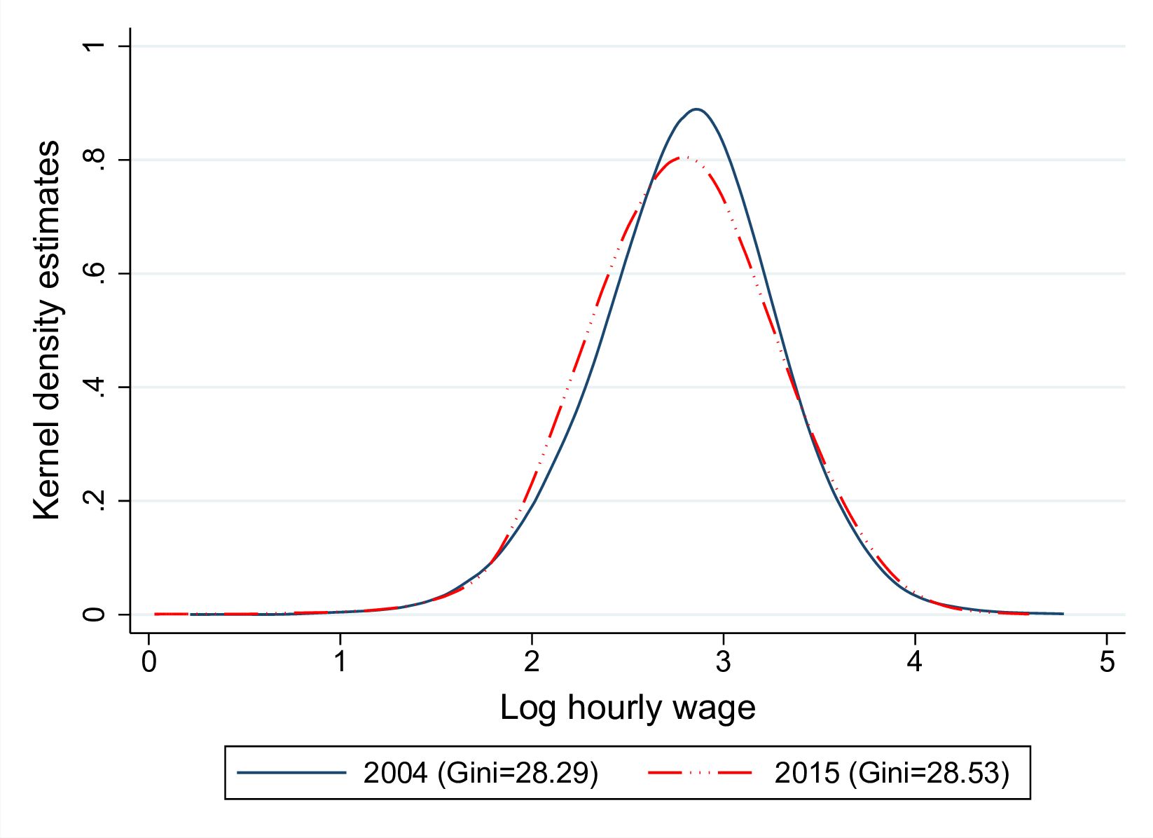
Inequality of paid wages in Germany increased strongly between 1990 and 2010. This trend was first driven by increasing wages of high incomes and since the mid 1990’s by decreasing real wages at the lower end of the income distribution (Dustmann et al., 2014; Card et al., 2013). Since 2011 this process has slowed down (Fitzenberger and Seidlitz, 2020; Möller, 2016). Figure 2 shows the growing spread of observed hourly wages between 2004 and 2015 accompanied by a small decrease of real wages due to an increasing number of employees earning low-wages.

Figure 2

Download asset Open asset

Kernel density estimate of log hourly wages for 2004 and 2015. Source: IAB-MSM; author’s own presentation.

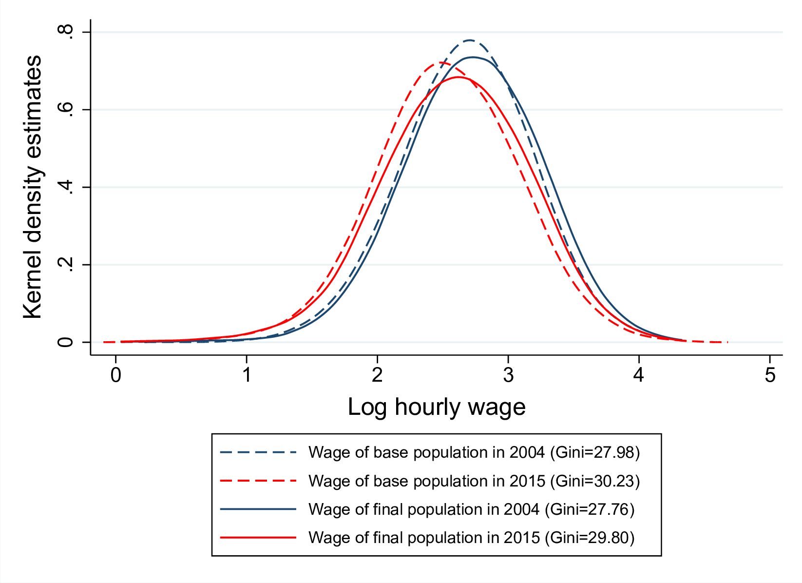
Figure 3 presents the wage distribution of predicted wages for the full population of flexible workers – including non-working but employable individuals – for 2004 and 2015 as well as their respective counterfactual distributions if the coefficient of the other periods’ estimation are used for prediction. The predicted distributions for all flexible workers confirm the picture of observed wages: The wage distribution in 2015 is flatter and slightly shifted to the left compared to 2004. An increase of wage inequality and decrease of real wages due to wage structure changes can be found for both, the final and base period population (comparing lines of the same type). This also indicates that the increase of observed wage inequality is not only due to composition changes of the workforce, but also the result of changes in the wage structure of a given population. Changes of the population between 2004 and 2015 increases wage inequality further, but shifts the wage distribution to the right (comparing lines of the same color). This wage increasing effect of composition changes is even stronger when measured at the 2015 wage structure.

Figure 3

Download asset Open asset

Simulated kernel density estimate of log hourly wages. Source: IAB-MSM; author’s own presentation.

The finding of increasing wage dispersion due to changes in the payment structure as well as compositional changes is consistent with findings in the literature. Drivers are the skill-bias in labor demand (Dustmann et al., 2009; Antonczyk et al., 2011) and changes in the composition of the workforce accompanied by the increase of employment (Dustmann et al., 2009; Biewen and Seckler, 2019). Besides population ageing and an expansion of education also the increase in heterogeneity of employment histories plays and important role (Biewen et al., 2018). The Hartz reforms are held responsible for the rise in low-wage employment (Bradley and Kügler, 2019; Hochmuth et al., 2021). Although the introduction of a general minimum wage in 2015 increased wages in the first wage decile significantly (Bossler and Schank, 2020; Fedorets et al., 2019), it has not yet fully counteracted the rise of low-wage employment (Fedorets et al., 2019). Using the SOEP data, Fedorets et al. (2019) show that a substantial share of workers in 2015 still earned less than the minimum wage. Non-compliance decreased in 2016, but rose again after an increase of the minimum wage in 2017 (Schröder et al., 2020).

3.3. Employment changes

Table 1 displays the simulated marginal employment effects per working hour category for men and women. The simulation finds a total increase in the number of employees between 2004 and 2015 by approximately 2.2 million (bottom left in Table 1), which represents an increase of approximately 8.2 percent compared to the 27.2 million simulated employed worker in 2004. Much of this increase is attributable to women: Female employment increases by 1.6 million or 12.1 percent. Measured in full-time equivalents, the overall increase of 1.8 million (bottom right in Table 1) and 7.4 percent is slightly smaller. Differences to the official employment figures are due to different definitions of employment. In addition, only main employment is considered in the simulation model. Further deviations may also occur due to the SOEP sample. Differences to Figure 1 appear due to self-employment and inflexible employees.

Table 1

Simulated employment changes per working hour category

Employment change in 1000		Working hour category							FTE
Partial effect		0	10	15	20	30	40	50	FTE
Base period	Men	2,073	42	26	125	281	11,312	2,105	14,237
	Women	5,375	1,228	664	2,203	2,074	6,581	561	10,496
	Total	7,448	1,270	690	2,328	2,355	17,893	2,667	24,734
Indirect policy	Men	$-$ −175	$-$ −18	−1	−5	−3	+126	+75	+210
	Women	$-$ −186	$-$ −56	$-$ −20	$-$ −3	+35	+198	+33	+242
	Total	$-$ −361	$-$ −74	$-$ −21	$-$ −8	+32	+324	+107	+452
Indirect wage	Men	+124	+11	+6	+8	+2	−84	−66	−156
	Women	+154	+26	+12	$-$ −10	$-$ −34	$-$ −121	$-$ −26	$-$ −174
	Total	+278	+36	+18	−2	−32	−206	−92	−330
Preference	Men	+156	+32	+27	+46	+115	−480	+105	$-$ −223
	Women	$-$ −490	$-$ −12	+15	+155	+749	−703	+285	+296
	Total	$-$ −334	+20	+43	+201	+864	−1183	+390	+73
Restriction	Men	$-$ −789	+22	+22	+35	+60	+574	+75	+744
	Women	$-$ −431	+42	+34	+90	+125	+130	+10	+304
	Total	$-$ −1220	+65	+56	+126	+186	+704	+84	+1049
Population	Men	+66	−20	−12	−41	−91	−320	+106	$-$ −286
	Women	−655	−269	+26	−361	+146	+873	+99	+869
	Total	−589	−289	+14	−402	+56	+553	+204	+582
Total changes	Men	$-$ −617	+27	+42	+43	+84	−185	+294	+289
	Women	−1,609	−269	+67	−128	+1,022	+377	+400	+1,537
	Total	−2,226	−242	+109	$-$ −85	+1,105	+192	+694	+1,826

Note: FTE = Full-time equivalent.
Source: IAB-MSM; author’s own calculation.

The indirect policy effect describes the employment adjustments due to tax or benefit changes. The simulation results suggest that the strong increase in employment between 2004 and 2015 is partly a consequence of changes in the tax and transfer system, making work, in particular full-time work, more attractive. Policy changes lead to an estimated increase of working individuals by approximately 360,000 (change in 0 working hour category due to indirect policy). In addition, policy changes have caused part-time employment of up to 20 hours to decline (total change in working hour categories 10, 15 and 20 due to indirect policy), so that the employment effect measured in full-time equivalents is even higher (+452,000, see column FTE of Table 1). This pattern is evident for men and women.

The analysis in Section 3.2 has shown that real hourly wages have decreased and dispersed between 2004 and 2015. The potential effect of decreasing hourly wages on labor supply is ambiguous: Decreasing real wages could lead to declining labor supply via the substitution effect or increasing labor supply via the income effect. With wage inequality growing at the same time, wage change varies across the income distribution, making an a priori assessment of the employment effect difficult. The simulation finds that employment decreased by about 280,000 workers (change in 0 working hour category) due to wage changes between 2004 and 2015. The results show a decline of jobs with higher volume of hours but a small increase in part-time jobs with few hours worked, resulting in a decrease of full-time equivalent workers by 330,000. The changes are very similar for women and men.

Simulated employment effects of preference changes on the other hand vary strongly between men and women. Labor market participation of women increases by 490,000 due to preference changes. The strong participation effect is related to an increase of women willing to work 20, 30 or 50 hours a week, while the number of women working 40 hours a week decreases. This pattern is quite similar for men, but the increase of male employment in part-time and overtime work do not equalize the decrease of full-time work. Preference changes lead to an overall decrease of male participation by 160,000 (change in 0 working hour category). Measured in full-time equivalents, male employment decreases by 220,000, while female employment increases by 300,000 full-time equivalents. The estimated preference effect is in line with findings by Blömer et al. (2021) about changes in desired working hours during this period. Changes of labor supply preferences can be caused by difference reasons. Direct drivers of preference changes are for example changes in the attitude toward the division of paid and unpaid labor within families and self-actualization goals of individuals and workers. Additionally, external and policy changes not covered by the tax and benefit function may affect labor supply preferences. Examples are the availability and costs of child care facilities or changes in obligations and work requirements for benefit recipients by Hartz IV. Changes in the number of available child care facilities are more likely to affect the preference than the restriction equation, since the possibility to take up work within the next four weeks is a condition for involuntary unemployment. This is usually not the case for parents without childcare options. The expansion of subsidized early child care during this period is therefore likely a main driver of increasing preferred working hours of women (Zimmert, 2019) as well as the female catch-up of educational attainments. Hartz IV did not only introduce the new benefit UB II, directly affecting the tax and transfer system, but also conditions for transfer receipt have been tightened, following the principles of promoting and demanding. Obligations to apply for jobs, participate in training, regular appointments at the job center and sanctions for the refusal of job offers likely led to the reduced attractiveness of non-employment and changed labor supply preferences (Bradley and Kügler, 2019; Burda and Seele, 2020; Hochmuth et al., 2021; Krebs and Scheffel, 2013).

The simulation shows that the reduction of labor market restrictions is the main reason for the employment boom between 2004 and 2015: involuntary unemployed decreased by almost 1.2 million (change in 0 working hour category). The reduction of labor market restrictions accounts for more than half of the overall employment upswing. With almost 790,000 additional workers, most of whom are employed full-time, men are the main beneficiaries of the reduction in labor market restrictions. However, also female employment increases by more than 430,000 over all working hour categories. Measured in full-time equivalents male employment rises by almost 750,000 and female employment by over 300,000 due to the decline of involuntary unemployment. Estimated involuntary unemployment decreases strongly from 9% in 2004 to 4% in 2015, which is close to the reduction of ILO unemployment rate from 10% to 4%. The decline can be observed across different subgroups, while differences in simulated involuntary unemployment rates between the subgroups persist. Improved matching efficiency in the wake of the labor market reforms plays a decisive role in the decline in the unemployment rate and the individual restriction probability (Hutter et al., 2022; Klinger and Rothe, 2012; Klinger and Weber, 2016; Launov and Wälde, 2016), changes in separation propensity and job creation intensity (Hartung et al., 2018; Klinger and Weber, 2016), and increased working hour flexibility (Bradley and Kügler, 2019; Carrillo-Tudela et al., 2018; Weber, 2015). The business cycle and technology shocks are of minor importance (Hutter et al., 2022; Klinger and Weber, 2019).

Population changes between 2004 and 2015 cause a further increase in employment by about 590,000 workers (change in 0 working hour category). Reasons for this could be differences in individual and household characteristics and the total number of working-age individuals between both samples. This is in line with the results of Hutter et al. (2022), who find that an expanding labor force explains part of the employment boom in Germany. Increasing employment due to population changes enters the other effect in the decomposition of income inequality.

Figure 4 presents the employment changes by deciles of household’ disposable income. This provides a first insight into the likely distributional impact of the partial effects. The employment growth due to labor supply adjustments to policy changes is distributed across the full income range, but being strongest in the first and lowest in the tenth decile. Also the employment reduction following wage changes does not show substantial differences across the income distribution. Employment declines in all deciles, but most sharply in the 20 percent of households with the lowest income. It is therefore reasonable to assume that the indirect policy and wage effects do not have a large impact on income inequality.

Figure 4

Download asset Open asset

Simulated employment changes per income decile and effect type. Note: The columns represent the employment change per households’ disposable income decile from first (left) to tenth (right) decile. Source: IAB-MSM; author’s own presentation.

Changes in preferences affect employment of high- and low-income households very differently. While employment in the lower income groups declines significantly as a result of preference changes, it rises significantly at the upper end of the income distribution. The previous analysis showed that women are joining and men withdrawing from the workforce due to preference shifts. This suggests that the additional women in the labor force mostly come from higher-income households and the men who leave the labor force come from lower-income households. In contrast, households from the lower end of the income distribution benefit in particular from the reduction in labor market restrictions. The analysis finds that a predominant portion of the employment growth occurs in the first five deciles. Households with higher income benefit as well from the reduction of labor market restrictions, but to a smaller extent.

3.4. Population changes

Differences in individual and household characteristics of the underlying populations may additionally affect the income distribution. The residual population effect captures all differences between the base and final period income distribution not explained by policy, wage and employment changes due to restriction and preference changes. Using a similar approach like the decomposition method applied in this paper, Jessen (2019) finds a strong inequality increasing effect of population changes between 2002 and 2011.

Table 2 shows descriptive statistics of the underlying populations. The upper part of the table shows some serious household changes: The number of single households¹⁴ and single parents, who face a high risk of poverty, increased strongly, while the number of couples with children decreased. Accordingly, the average household size declined from 2.07 persons per household in 2004 to 1.96 person in 2015. Table 2 shows in particular a remarkable increase in one-person households. Peichl et al. (2012) show that decreasing household sizes increase inequality. Additionally, less obvious changes in household compositions like assortative mating may affect disposable income inequality (Blundell et al., 2018).

Table 2

Population changes

	2004	2015
Household characteristics
Household type
Singles	39.69%	46.39%
Single parents	9.20%	10.05%
Couples without children	28.42%	27.06%
Couples with children	22.70%	16.50%
Household size
1 person	38.30%	41.88%
2 persons	33.81%	34.05%
3 persons	14.38%	13.97%
4 persons	9.98%	7.73%
5 or more persons	3.53%	2.37%
Individual characteristics
Age
0 - 16 years	17.50%	15.34%
17 - 65 years	63.42%	62.62%
> 65 years	19.08%	22.04%
Nationality (of adults)
German	92.40%	90.90%
Other	7.60%	9.10%
Educational degree (25 - 65 years)
Low degree	37.25%	25.66%
Medium degree	39.78%	43.50%
High degree	22.97%	30.84%
Vocational degree (25 - 65 years)
Vocational degree	86.28%	85.85%
No vocational degree	13.72%	14.15%
Employment status (25 - 65 years)
Blue collar	23.36%	17.92%
White collar	35.66%	48.42%
Self-employed	6.56%	6.03%
Civil servant	4.45%	4.81%
Not employed	29.29%	21.58%
Other	0.68%	1.24%

IAB-MSM = author’s own calculation;
Note: Population shares after household selection with adjusted SOEP weights.

The lower part of Table 2 presents change in individual characteristics between base and final period. Population aging results in a larger share of people of retirement age and a decreasing share of minors and adults in working age. Although the special migration patterns due to the humanitarian crisis starting in 2015 are not reflected by the data, the share of non-German already increased between 2004 and 2015.

While the wage effect captures inequality changes due to changes in the hourly wages of a given population, differences in the wage distribution resulting from differences in potential wages of the underlying populations, comparable to the endowment effect of an Oaxaca-Blinder decomposition, are reflected by the population effect. Section 3.2 shows that additional to the payment structure also population differences between 2004 and 2015 explain changes in simulated hourly wages. Key drivers of individual wage potential are education and employment type. Between 2004 and 2015 the share of better educated individuals increased strongly. However, also the share of working age individuals without any vocational degree increased. Regarding the employment status we also see some serious shifts between base and final period population potentially affecting the income distribution. White collar work increased strongly while the share of blue collar workers and not employed people decreased. While the share of self-employed remained relatively constant, they face a slight increase of poverty risks. Most of the difference in the number of not employed can be explained by changes in labor supply due to policy, wage and preference changes as well as restriction changes. However, as Table 1 has shown, population changes further increased employment by almost 600,000. The resulting changes in inequality are captured by the population effect. Biewen and Sturm (2022) find an inequality increase due to changes in individual characteristics. This is also in line with findings in the literature that address a notable share of rising wage inequality in individual wage potentials (Dustmann et al., 2009; Biewen and Seckler, 2019).

Besides the presented changes in household and individual characteristics, the residual population effect captures other changes which may be not discussed here like further population changes, differences in non-labor income, Biewen and Sturm (2022) find no relevant change in capital incomes, and the distribution of income from self-employed. However, the descriptive summary of changes in some important characteristics in this section already shows that population trends may well affect the distribution of household disposable income significantly.

4. Results

4.1. Changes in inequality

Changes in employment and wages affect disposable household income via gross income changes. Therefore, it is insightful to take a look at changes of gross income first before analyzing the changes in disposable income inequality. Looking at the distribution of positive households’ gross income, the simulation finds a strong increase in inequality between 2004 and 2015. Table 3 presents the results for the decomposition of gross income of households from employment.

Table 3

Decomposition results: Percentage change in inequality of gross household income from employment

Inequality change
Partial effect	Gini	Atkinson	P90/P10	P90/P50	P50/P10
Indirect policy	-1.14%	-1.27%	-2.81%	-0.64%	-1.95%
Wage	+2.56%	+7.47%	+7.79%	+2.64%	+4.72%
Indirect wage	+1.27%	+0.61%	+1.27%	+0.32%	+0.86%
Preference	+0.76%	+5.73%	+8.95%	+2.14%	+6.38%
Restriction	-4.33%	-0.22%	-0.27%	-0.39%	+0.11%
Population	+2.89%	+5.21%	+3.94%	+5.18%	-1.31%
Total employment	-3.44%	+4.85%	+7.14%	1.43%	+5.40%
Total change	+2.01%	+17.52%	+18.88%	+9.25%	+8.81%

Note: Inflexible households are excluded. For Atkinson and percentile ratios households without income from employment are excluded.
The five columns present the Shorrock-Shapley value of the change in inequality measured with the Gini-coefficient, the Atkinson-index with inequality aversion parameter ∈ = 0.5, and the ratios between the 90th and 10th, the 90th and 50th, and the 50th and 10th income percentiles in percent.
Source: IAB-MSM; author’s own calculation.

The simulation finds a widening spread of households’ gross income inequality between 2 percent, measured by the Gini-coefficient, and almost 19 percent when looking at the ratio between the ninth and first deciles. The strong difference between the Gini-coefficient and the Atkinson-coefficient and quantile ratios is partly due to the fact, that households without income from employment are incorporated when calculating the Gini-coefficient but not in the calculation of the other measures.¹⁵

Changes in income tax and transfers do not directly affect gross income, but determine the calculation of net income for a given gross income. Therefore, the effect of policy changes on gross income is null. The increase in gross income inequality due to changes of the payment structure reflects the findings discussed in section 3.2. Employment changes in total have an ambiguous effect on inequality of gross income, depending on the applied measure. While employment changes reduce the Gini-coefficient, percentile ratios and the Atkinson index increase. An important difference is the inequality decreasing restriction effect, which plays a bigger role when considering zero incomes. Labor supply changes have a mixed effect on inequality: The indirect policy effect, resulting from labor supply reactions to the transformation of gross into disposable income, reduces inequality of gross working income slightly. The employment reduction following wage changes, the indirect wage effect, have the opposite effect. The increase in employment due to preference changes leads to an increase in gross income inequality. While the reduction of involuntary unemployment, the restriction effect, reduces inequality. A large share of the overall increase in inequality in gross income is explained by changes in the population. The percentile ratio suggests that these changes play an important role, especially at the tails of the distribution. Overall, between 2004 and 2015 inequality of gross labor income increased significantly.

Looking at the change in disposable household income, a different picture emerges. While the overall change in inequality measured by the Gini coefficient is similar for gross ( $+$ 2.0 percent) and disposable ( $+$ 2.3 percent) household income, it is much smaller for disposable income and even becomes negative when measured by the Atkinson-index (-1.5 percent) or percentile ratios (between -3.3 and +1.8 percent). Changes in gross income are not necessarily accompanied by corresponding changes in disposable income. The redistribution through the tax and benefit system stabilizes the distribution of disposable income and attenuates changes in market income (Doorley et al., 2021; Paulus and Tasseva, 2020). This automatic stabilization was particularly strong in Germany during the Great Recession and the resulting European sovereign debt crisis (Dolls et al., 2022). Differences between market income and disposable income may also result from differences in the samples studied that are due to inflexible households.

Table 4 presents the decomposition results for households’ disposable income. Compared to the gross income distribution the simulated overall change in disposable income inequality is small, but the decomposition shows that the total change masks several opposing trends. Policy changes do not have an direct effect on gross income, but cause a reduction in the inequality of household’s disposable income. This is in line with the findings of Jessen (2019) and Biewen and Sturm (2022). The changes in tax and benefits lead to a sizeable decrease. Although no major income tax reform has taken place, taxation is relevant due to bracket creep in addition to transfer changes. Corresponding to the literature, this analysis finds an increase in inequality of the hourly wages and subsequently households’ gross income. However, the redistribution of the tax and benefit system cushions this effect to a large extent, so that only a negligible increase in inequality of disposable household income due to wage changes remains. This is consistent with the findings of Biewen and Sturm (2022), who also provide evidence that changes in the payment structure only play a minor role for disposable income inequality changes. However, this result deviates from Jessen (2019), who finds a significant inequality-reducing effect of wage changes between 2002 and 2011.

Table 4

Decomposition results: Percentage change in inequality of disposable household income

Inequality change
Partial effect	Gini	Atkinson	P90/P10	P90/P50	P50/P10
Policy	-2.30%	-2.91%	-3.33%	-2.39%	-1.07%
Indirect policy	-0.57%	-1.46%	-0.47%	+0.01%	-0.47%
Wage	+0.04%	+0.16%	+0.00%	+0.00%	+0.00%
Indirect wage	+0.38%	+0.65%	-0.06%	-0.01%	-0.05%
Preference	+0.65	+0.32%	-1.42%	-0.01%	-1.41%
Restriction	-1.84%	-3.72%	+0.10%	-0.02%	+0.11%
Population	+6.31%	+6.47%	+8.27%	+4.66%	+3.80%
Growth	-0.34%	-0.97%	-4.70%	-0.47%	-4.25%
Total employment	-1.38%	-4.21%	-1.85%	-0.03%	-1.81%
Total change	+2.33%	-1.46%	-1.62%	+1.78%	-3.34%

Note: The five columns present the Shorrock-Shapley value of the change in inequality measured with the Gini-coefficient, the Atkinson-index with inequality aversion parameter ∈ = 0.5, and the ratios between the 90th and 10th, the 90th and 50th, and the 50th and 10th income percentiles.
Source: IAB-MSM; author’s own calculation.

In total, employment changes reduce inequality of disposable income. However, as the decomposition reveals, the partial effects do not uniformly affect the distribution of disposable income. Labor supply adjustments following policy changes, the indirect policy effect, reduce inequality slightly. The indirect wage effect counteracts this partially. Increasing employment due to preference changes has different impacts on inequality depending on the applied measure of inequality: Gini- and Atkinson-index rise, while the percentile ratios decline. The strong employment increase by 1.2 million due to restriction changes results in a decrease of disposable income inequality measured by Gini- and Atkinson-index. However, the effect of less involuntary unemployment on the percentile ratios is negligible.

The decrease of inequality due to policy and employment changes is overcompensated by a strong increase of inequality due to population changes when looking at the Gini-coefficient. Comparable to Jessen (2019) for the period 2002 to 2011, a remarkable inequality increasing residual effect remains.

4.2. Effect heterogeneity: estimation results

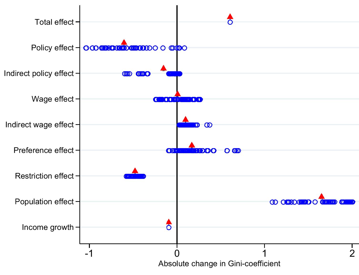
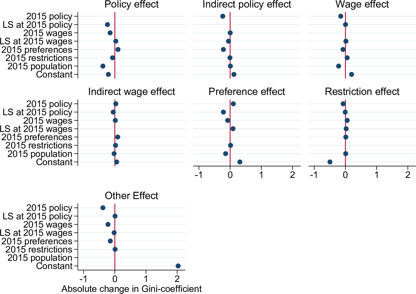
Figure 5 shows the simulated effects of each decomposition of the inequality change measured by the Gini-coefficient together with the Shorrocks-Shapley value. It becomes apparent that the simulated results, with the exception of the indirect wage and restriction effect, diverge strongly depending on the underlying population. This is in line with the results of O’Donoghue (2021), who also finds considerable differences between different decomposition paths. To gain further insight into how differences in the population affect the estimated effects, I regress each simulated effect on a series of binary variables indicating if the characteristics of the underlying counterfactual population are from the base or final period. The estimation is performed on the 64 different combinations of final and base period characteristics, not on the 5,040 permutations, so that each underlying population is considered only once.

Figure 5

Download asset Open asset

Decomposition of change in Gini-coefficient. Note: The triangles mark the Shorrocks-Shapley Value of each effect. Each circle represents one different decomposition.Source: IAB-MSM; author’s own presentation.

Figure 6 shows the estimation results for each of the seven factors.¹⁶ The constant represents the respective effect estimated on base period characteristics. The coefficients can be interpreted as the interaction effect of the two partial effects (dependent and independent variable) on inequality.

Figure 6

Download asset Open asset

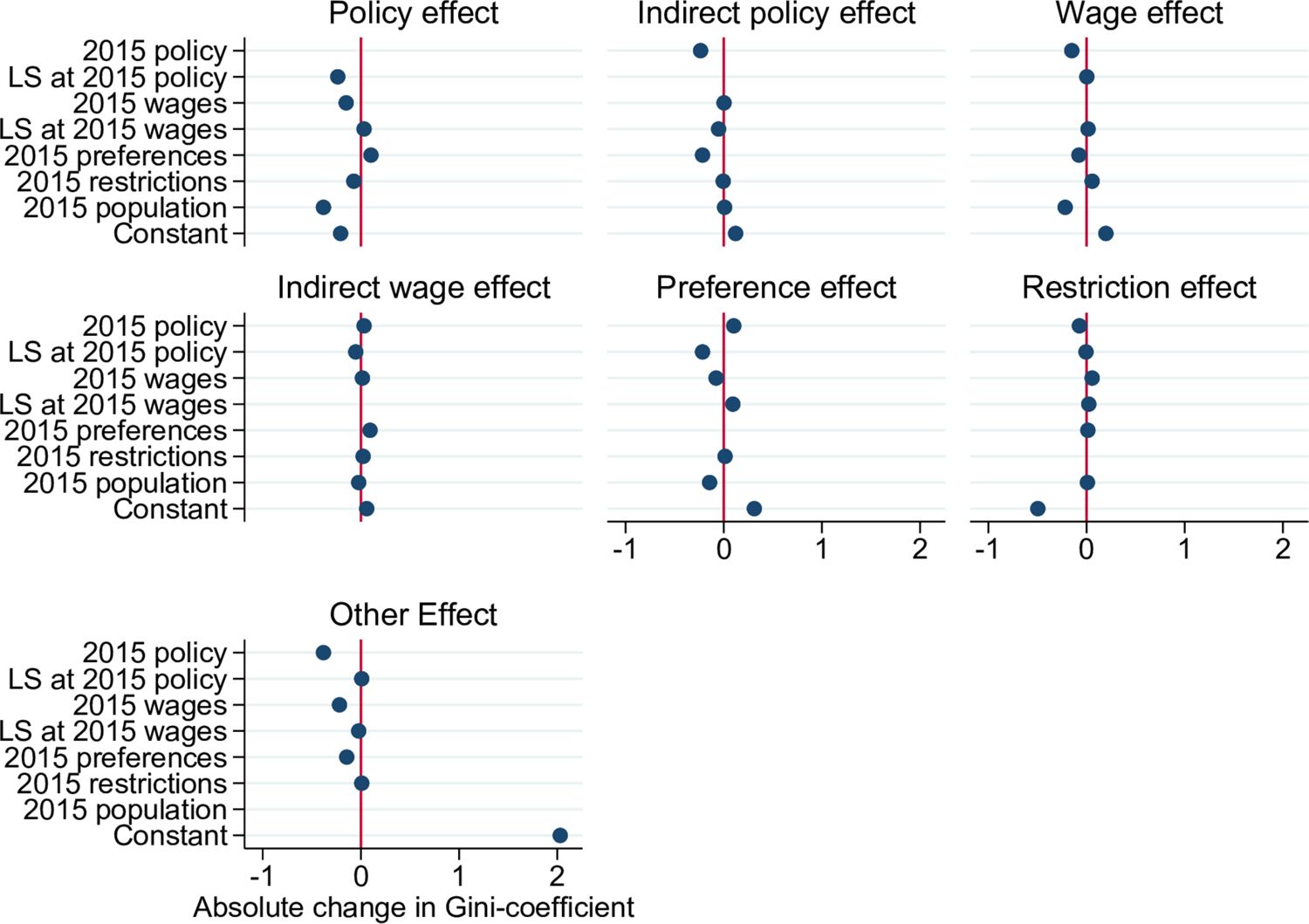
Effect heterogeneity. Note: The effect changes are estimated on all 64 possible counterfactual distributions. The constant describes the average effect size when measured at the base period situation.Source: IAB-MSM; author’s own presentation.

The policy effect is quite unstable depending on the underlying scenario. The equalizing effect of policy changes is stronger when considering accompanying labor supply adjustments and measuring at wages, restrictions and the population of 2015. That implies that policy changes and subsequent labor supply adjustments are mutually reinforcing. This is presumably the case because labor supply adjustments are achieved by supporting the financial situation of those who have adjusted their labor supply at the lower end of the income distribution.

The indirect policy effect on inequality also varies substantially over the decomposition paths. When simulation the effect with base period characteristics, it even changes its direction. Not only does the underlying policy alternate the indirect policy effect, also changing preferences significantly reduce it. The small effect of wage changes turns negative when evaluated at policy and population of 2015. Preference and restriction changes work slightly in the opposite direction. The indirect wage effect differs only slightly between underlying characteristics of base and final period.

The inequality amplifying preference effect estimated at the base period is about twice the size of the average over all decompositions. Labor supply adjustments to policy, wage changes and the final period population reduce the effect of preference changes significantly, while policy changes and behavioral adaptions to wage changes work in the opposite direction. The levelling effect of restriction changes is found across all underlying scenarios. The strong effect of population changes gets smaller when considering policy, wage and preference changes.

The analysis of effect heterogeneity shows that it is important to estimate the impact of particular changes on more than just the base or final period population to avoid biased conclusions. This is not only relevant for the review of decomposition studies, but also important to keep in mind when designing policy changes or discussing the transfer of successful reforms between countries.

5. Conclusion

This paper applies a decomposition framework using behavioral microsimulation to identify the role of the ‘German job miracle’ on inequality in disposable household income between 2004 and 2015. This period is characterised by a variety of factors possibly influencing the inequality of disposable household income. These include a big welfare reform in the beginning, the financial and economic crisis in between as well as a long lasting labor market upswing and changes of the population structure.

Previous decomposition studies for Germany have examined the role of changing employment in disposable income changes. However, they lack differentiation between the underlying causes of employment growth (Biewen and Juhasz, 2012; Biewen et al., 2019; Biewen and Sturm, 2022; Haupt and Nollmann, 2014). The utilized approach extends the framework of Bargain (2012) and Jessen (2019) by the usage of a double hurdle model of labor supply. It is the first analysis that identifies the effects of employment changes due to labor supply preferences and labor market constraints and isolates employment changes due to policy and wage changes. Additionally, direct effects of policy and wage changes on inequality are considered. Hence, this paper adds another piece to ‘Germany’s inequality puzzle’ (Biewen and Sturm, 2022).

The simulation finds that the increase in employment is driven by changes in labor supply preferences as well as a reduction of labor market restrictions. Labor supply adjustments to policy and payment structure changes largely cancel each other out. While the increase in employment due to changes in preferences is exclusively accounted for by women, men benefit more from the strong employment growth due to eliminated restrictions.

The results show why inequality has remained relatively stable between 2004 and 2015 despite this remarkable increase in employment. Across the income distribution, households have increased their labor supply, so the overall income distribution has consequently not changed significantly. In contrast, the reduction of labor market restrictions has a particular strong impact on employment of low income households and therefore reduces inequality significantly. Additionally, changes in the tax and benefit system have led to a stronger redistribution of disposable income. However, changes in the population, including changes in income-related characteristics and thus in the wage potential of the population, counteract employment and policy changes and lead to a small overall increase in inequality. Changes in the wage structure itself increase inequality of pre-tax household income but do not affect the dispersion of disposable income. Without policy adjustments and the elimination of labor market restrictions, Germany would have seen a further increase in income inequality between 2004 and 2015 due to changes in population. An important question beyond the scope of this paper is how population changes will affect income distribution in the future, which should be analyzed by using a dynamic framework.

The strong effect of population changes on inequality highlights the importance of redistributing measures if politics intends to stabilize, or even reduce, inequality. Between 2004 and 2015, the reduction of labor market restrictions, along with policy changes, offset this trend. This remarkable employment effect is not repeatable, as involuntary unemployment is already at a low level and – as this study shows – incentives aiming at increasing labor supply do not necessarily decrease inequality. Therefore, redistributive policies are likely to play an even greater role in maintaining the level of inequality in Germany in the future if inequality increasing population changes continue. However, as the comparison of gross and disposable income changes has shown, the German tax and benefit system attenuates inequality of market incomes and automatically stabilizes the income distribution.

The cross-sectional perspective of the applied framework does not consider the effects of employment changes on inequality over the life-cycle. Women’s employment, in particular, is important to compensate for poverty and income disparities in old age or when life situations change, for example after a separation. In this respect, the positive employment effects due to preference changes may also be able to reduce inequalities in the long run, even if they initially increase inequality. The inter-temporal perspective of the ‘German job miracle’ and its impact on inequality are beyond the scope of this paper and might be the subject of future research.

Contrary to related decomposition studies, in this analysis the partial effects are not only evaluated at the base or final period situation or one counterfactual distribution in between, but on the full set of possible permutations following the suggestion of Bargain and Callan (2010). The findings illustrate that the simulation results differ notable with the underlying population. An evaluation based on only one distribution might lead to biased conclusions. Furthermore, this emphasizes the importance to consider the properties of a population when designing policy changes or discussing the transfer of successful reforms between countries.

Footnotes

1.

See Goebel et al. (2018) for a documentation on the SOEP.

2.

Table A1 in the Appendix shows the number of affected households at each selection step.

3.

The model is estimated with the user written command lslogit developed by Max Löffler in Stata.

4.

This specification ignores a possible correlation between unexplained differences of unemployment risks and preferred working hours, for example unobservable discouragement effects (Bargain and Callan, 2010).

5.

The extension for couple household is straightforward. The probabilities for all different labor states of couples are shown in Appendix A3.

6.

Alternatively nominal wage increase can be used as uprating parameter. See for example Bargain and Callan (2010). A discussion of the uprating parameter can be found in Bargain and Callan (2010) and Bargain (2012). Sutherland et al. (2008) provides an overview over different uprating strategies governments use and their effects on income and poverty.

7.

The housing benefit (Wohngeld) is not linearly homogeneous in its parameters. Therefore, the applied uprating strategy of the housing benefit differs: The benefit is first calculated according to the respective regulations and is up- or downrated afterwards.

8.

Bruckmeier and Wiemers (2018) show that the non-take-up of benefits in Germany is not negligible. The proposed simulation procedure assumes full take-up of transfer benefits, which lowers the level of inequality but do not distort the decomposition results if take-up rates do not change systematically over time.

9.

Log hourly wages are regressed on years of education, years worked in full-time and part-time employment, tenure, age, German nationality, marital status, and age and number of children in the household. The number of years not worked within the last 10 years controls for human capital depreciation and a Berlin dummy accounts for the difference in wages between Berlin and the other East German states. Categorical education variables, work experience, years without employment in the last 10 years, age categories, marital status, age and number of children living in the household, degree of disability and the income of other household members serve as exclusion restrictions. For each period, four estimations are run separately for women and men in East and West Germany. See estimation tables A4–A7.

10.

Tables A9–A13 in the Appendix present the estimation results of the preference model for different household types in the base and final period.

11.

Table A8 in the Appendix presents the results of the restriction estimation for men and women in both periods.

12.

Each effect is measured on 64 different underlying populations. In total 128 counterfactual scenarios are simulated and 5,040 different (factorial 7) decompositions are calculated. The income growth effect is small and of minor interest for the analysis. Therefore, it is solely estimated on the basis of the base period population. This reduces the number of necessary simulations by half and the number of possible permutations to one eighth.

13.

For more details on the Hartz IV reform and its impact on different households budgets see Arntz et al. (2007), Becker and Hauser (2006), Blos and Rudolph (2005), and Schulte (2004) or Bradley and Kügler (2019) for a recent evaluation.

14.

Single households are defined as households in which the head of household does not have a partner in the same household. Thus, a single household is not necessarily a one-person household.

15.

The total increase of gross income inequality measured by the Gini-coefficient calculated without zero incomes is 8.65 percent.

16.

Table A14 presents the respective estimation tables.

17.

To simplify the notation, I omit the index for the households.

18.

Following the definition of the International Labor Organization non-working individuals are considered involuntary unemployed if they searched for a job within the last four weeks and are able to start working within the next two weeks.

Appendices

A. Technical appendix

A.1. Household selection

Table A1

Household selection

Selection step	2004		2015
	N	$\Delta$	N	$\Delta$
Initial number of private households in GSOEP	11,795	(-)	15,996	(-)
Exclusion of households without interviewed head of HH and/or partner	11,721	74	15,952	44
Exclusion of couple households with survey non-response of partner	11,067	654	14,051	2,126
Households interviewed in the simulation year and the following year	9,905	1,162	11,614	1,433
Exclusion of households with missing information on worked hours, wages and other income variables	9,112	972	8,949	3,972
Excluded households	728		1,945
Households considered for income simulation	9,112		10,594
Households considered for inequality analysis	11,067		14,051

Note: N = remaining number of households, $\Delta$ = change in numbers of households in the respective selection step. Exclusions are overestimated, if one simply counts the households affected by a certain condition, since households may be affected more than once.
Source: IAB-MSM; author’s own presentation.

A.2. Double hurdle labor supply model

The discrete hours approach supposes that agents choose the utility maximizing number of working hours, $h$ , with $h\in\{h_{0},h_{1},h_{2},\ldots,h_{J}\}$ and $h_{0}=0$ , i.e., subject to the constraint that only a discrete number $J+1$ of hours categories (including zero hours) is available (couples choosing from a set that includes all combinations of choices of both partners).¹⁷ Each choice is associated with a specific net income, depending on the individuals’ hourly gross wage rate $w$ , household characteristics and the design of the tax and benefit system. The IAB-MSM computes the disposable income at all hour categories for each household. This allows to estimate the parameters of a utility function. Utility is assumed to increase in its arguments leisure $L$ and consumption $C$ , bounded by the time endowment $T$ and the budget constraint. The deterministic utility $V$ derived from choice $h$ is given by $V\left(h\right)=v\{\tau\left(wh,I\mid X\right),T-h\mid Z\}$ where the function $\tau(\cdot)$ refers to the tax-transfer rule transforming gross earned income $w h$ and exogenous non-labor income $I$ into disposable income. Relevant characteristics $X$ of the individual and household for the calculation of disposable income (e.g., marital status, number and age of children in the household) are considered in $\tau(\cdot)$ . Systematic taste shifters $Z$ regarding the preference for consumption and leisure (e.g., age, education and children in the household) are captured in the utility function $v(\cdot)$ . In order to capture unobserved utility components, which stem from the existence of unobserved preference characteristics and optimization or measurement errors, a random variable $\varepsilon$ is added to the deterministic utility function. The utility derived from working $h$ hours is the sum of deterministic utility $V$ and the random component $\varepsilon$ . Assuming a (type I) extreme-value distribution for $\varepsilon$ leads to the choice probabilities of the multinomial or conditional logit model (McFadden1974),

P (h) = \frac{\exp v {τ (w h, I ∣ X), T - h ∣ Z}}{\sum_{j = 0}^{J} \exp v {τ (w h_{j}, I ∣ X), T - h_{j} ∣ Z}} .

The unrestricted model assumes that each person is free to choose their preferred working hour category. Demand side constraints and involuntary unemployment are not considered, as each observed number of working hours is interpreted as the utility maximizing labor supply choice. In contrast, a double hurdle model of labor supply accounts for labor market constraints. It uses information on desired working hours (part-time or full-time) of involuntary unemployed.¹⁸ In this approach, the desired instead of the actual working hours are applied to model (1). The probabilities of choice categories with positive working hours are then multiplied by individual restriction risks. The latent equation of involuntary unemployment of each person is given by a stochastic function of characteristics $X$ that likely affect involuntary unemployment:

R^{*} = β X + υ .

The matrix $X$ includes individual characteristics as age, education and employment history but also the regional unemployment rate to consider for heterogeneity in labor market conditions. The assumption of normality of random term $\upsilon$ allows to estimate the restriction probability with a standard probit model. Table A8 presents the results of the estimation of unemployment probabilities.

A.3. Probabilities of labor market states for couples

1) Man and woman voluntary unemployed

P_{i}^{N P_{m} N P_{f}} = \frac{\exp (U_{i 0})}{\sum_{j = 0}^{J} \exp (U_{i j})},

2) Man involuntary unemployed and woman voluntary unemployed

P_{i}^{U E_{m} N P_{f}} = ϕ_{m} (β X) \sum_{k \in (h_{m} §gt; 0, h_{f} = 0)}^{J} \frac{\exp (U_{i k})}{\sum_{j = 0}^{J} \exp (U_{i j})},

3) Man voluntary unemployed and woman involuntary unemployed

P_{i}^{N P_{m} U E_{f}} = ϕ_{f} (β X) \sum_{k \in (h_{m} = 0, h_{f} §gt; 0)}^{J} \frac{\exp (U_{i k})}{\sum_{j = 0}^{J} \exp (U_{i j})},

4) Man and woman involuntary unemployed

P_{i}^{U E_{m} U E_{f}} = ϕ_{m} (β X) ϕ_{f} (β X) \sum_{k \in (h_{m} §gt; 0, h_{f} §gt; 0)}^{J} \frac{\exp (U_{i k})}{\sum_{j = 0}^{J} \exp (U_{i j})},

5) Man employed and woman voluntary unemployed

P_{i}^{E M P_{m} N P_{f}} = (1 - ϕ_{m} (β X)) \sum_{k \in (h_{m} §gt; 0, h_{f} = 0)}^{J} \frac{\exp (U_{i k})}{\sum_{j = 0}^{J} \exp (U_{i j})},

6) Man voluntary unemployed and woman employed

P_{i}^{N P_{m} E M P_{f}} = (1 - ϕ_{f} (β X)) \sum_{k \in (h_{m} = 0, h_{f} §gt; 0)}^{J} \frac{\exp (U_{i k})}{\sum_{j = 0}^{J} \exp (U_{i j})},

7) Man employed and woman involuntary unemployed

P_{i}^{E M P_{m} U E_{f}} = (1 - ϕ_{m} (β X)) ϕ_{f} (β X) \sum_{k \in (h_{m} §gt; 0, h_{f} §gt; 0)}^{J} \frac{\exp (U_{i k})}{\sum_{j = 0}^{J} \exp (U_{i j})},

8) Man involuntary unemployed and woman employed

P_{i}^{U E_{m} E M P_{f}} = ϕ_{m} (β X) (1 - ϕ_{f} (β X)) \sum_{k \in (h_{m} §gt; 0, h_{f} §gt; 0)}^{J} \frac{\exp (U_{i k})}{\sum_{j = 0}^{J} \exp (U_{i j})},

9) Man and woman employed

P_{i}^{E M P_{m} E M P_{f}} = (1 - ϕ_{m} (β X)) (1 - ϕ_{f} (β X)) \sum_{k \in (h_{m} §gt; 0, h_{f} §gt; 0)}^{J} \frac{\exp (U_{i k})}{\sum_{j = 0}^{J} \exp (U_{i j})} .

A.4. Income components

Table A2

Components of net household income in the IAB-MSM

Model stage		Income components	Determined in tax and transfer module?
1		Earned income	no
	+	Self-employed income	no
	+	Capital income	no
	+	Rental income	no
	+	Other income sources (pensions)	no
2	-	Social security contributions	yes
	-	Income tax	yes
	-	Alimony payments	yes
3	+	Child benefit	yes
	+	Child-raising allowance	yes
	+	Unemployment benefits	yes
	+	Federal student support, stipends, claims to maintenance, widow’s allowance, maternity allowance, reduced hours compensation	no
4	+	Housing allowance	yes
	+	Supplementary child allowance	yes
	+	Social assistance for employable persons (SGB II)	yes
	+	Social assistance for unemployable persons (SGB XII)	yes
	=	Net household income	yes

A.5. Policy parameter

Table A3

Policy parameter

Policy parameter	2004	αρ2004	2015
Benefits
Unemployment Benefit (share of previous net income)	60% (67%)*		60% (67%)*
Unemployment Assistance (share of previous net income)	53% (57%)*
Social Assistance	291€̂	349€	404€
Unemployment Benefit II			404€
Income tax
Marginal tax burden in 1st progressive zone	16% - 24.05%		14% - 23.97%
Marginal tax burden in 2nd progressive zone	24.05% - 45%		23.97% - 42%
Marginal burden in 1st linear zone	45%		42%
Marginal burden in 2nd linear zone (rich tax)			45%
Basic tax allowance	7,664€	9,187€	8,472€
Lower threshold of 2nd progressive zone	12,739€	15,271€	13, 469€
Lower threshold of 1st linear zone	52,151€	62,515€	52,881€
Lower threshold of 2nd linear zone (rich tax)			250,730€
Social security contributions
Contributions to statutory pension insurance	19.5%		18.7%
Contributions to statutory unemployment insurance	6.5%		3.0%
Contributions to statutory health insurance	14.2%		15.5%
Contributions to statutory long-term care insurance	1.7%		2.6% (2.35%)*
Upper threshold of marginal employment (SSC free jobs)	400€	479€	450€
Upper threshold of contributions to statutory pension insurance	5,150€ (4,350€)̂*	6,173€ (5,214€)̂*	6,700€ (6,150€)̂*
Upper threshold of contributions to statutory unemployment insurance	5,150€ (4,350€)̂*	6,173€ (5,214€)̂*	6,700€ (6,150€)̂*
Upper threshold of contributions to statutory health insurance	3,488€	4,181€	4,125€
Upper threshold of contributions to statutory long-term care insurance	3,488€	4.181€	4,125€

Note: The Table includes only the most important policy parameter. Uprating parameter $\alpha$ is set to 1.1987 according to consumer price inflation between 2004 and 2015.
∗ with children.
∗∗ unweighted average over all federal states.
∗∗∗East Germany.
Source: IAB-MSM; author’s own presentation.

B. Estimation tables

Table A4

Estimation results for wage equation of men in East Germany

	2004		2015
	b	se	b	se
Log hourly wages
Years in education	0.0603 ${}^{***}$	(0.0068)	0.0951 ${}^{***}$	(0.0055)
Full-time	-0.0157 ${}^{*}$	(0.0061)	0.0011	(0.0041)
Part-time	-0.0228 ${}^{**}$	(0.0084)	-0.0060	(0.0062)
Human capital dep.	-0.2667 ${}^{***}$	(0.0627)	-0.0622	(0.0654)
Human capital dep. sq.	0.0691 ${}^{***}$	(0.0209)	-0.0438	(0.0318)
Tenure	0.0116 ${}^{*}$	(0.0048)	0.0198 ${}^{***}$	(0.0039)
Tenure sq.	-0.0180	(0.0121)	-0.0216	(0.0112)
Age	0.1133 ${}^{*}$	(0.0496)	0.0444	(0.0510)
Age sq.	-0.2132	(0.1186)	-0.0576	(0.1219)
Age cub.	0.1496	(0.0920)	0.0065	(0.0931)
Married	0.0812 ${}^{*}$	(0.0382)	0.0693 ${}^{*}$	(0.0319)
Separated	0.1510 ${}^{*}$	(0.0733)	0.0363	(0.0969)
Divorced	0.0744	(0.0478)	0.0561	(0.0484)
Children 0-3	-0.0035	(0.0443)	-0.0413	(0.0386)
Children 4-6	0.0346	(0.0502)	0.0618 ${}^{*}$	(0.0315)
Berlin	0.1924 ${}^{***}$	(0.0401)	0.0841 ${}^{**}$	(0.0326)
Constant	-0.1285	(0.6634)	0.3731	(0.6789)
Selection
Low education	0.4902	(0.6294)	0.6708	(0.5615)
Medium education	0.8935	(0.6048)	0.4006	(0.4904)
High education	-1.1962	(0.6265)	-0.5408	(0.5210)
Vocational degree	1.1709 ${}^{*}$	(0.5873)	0.8428	(0.4529)
University degree	1.6311 ${}^{**}$	(0.5976)	0.4673	(0.4678)
Experience	0.0468 ${}^{*}$	(0.0192)	-0.0093	(0.0139)
Human capital dep.	-1.9419 ${}^{***}$	(0.1342)	-1.5065 ${}^{***}$	(0.1313)
Human capital dep. sq.	0.2821 ${}^{***}$	(0.0338)	0.1424 ${}^{***}$	(0.0327)
Age 26-30	0.3566	(0.2406)	1.0566 ${}^{***}$	(0.2412)
Age 31-35	0.3749	(0.2898)	1.0539 ${}^{***}$	(0.2741)
Age 36-40	0.0762	(0.3671)	1.4974 ${}^{***}$	(0.2935)
Age 41-55	-0.2919	(0.4088)	1.5560 ${}^{***}$	(0.3563)
Age 46-50	-0.3446	(0.5127)	1.5454 ${}^{***}$	(0.3789)
Age 51-55	-0.3164	(0.5918)	1.5913 ${}^{***}$	(0.4496)
Age 56-60	-1.2568	(0.6874)	1.6276 ${}^{**}$	(0.5054)
Age 61-65	-2.1426 ${}^{**}$	(0.8132)	0.4614	(0.5823)
Married	0.0600	(0.1564)	0.2883 ${}^{*}$	(0.1353)
Separated	-0.3616	(0.2619)	-0.3547	(0.2593)
Divorced	-0.3332	(0.2135)	-0.2595	(0.2101)
Children 0-3	0.2660	(0.2056)	0.1530	(0.1789)
Children 4-6	0.3129	(0.2041)	0.0436	(0.1529)
kind16	0.1424	(0.1390)	0.1742	(0.1301)
kind17	0.0792	(0.2264)	-0.2543	(0.2935)
Disability	0.0049	(0.0035)	-0.0069	(0.0035)
Other income	-0.8729 ${}^{***}$	(0.1037)	-0.4768 ${}^{***}$	(0.0610)
Other income sq.	0.8984 ${}^{***}$	(0.1605)	0.2678 ${}^{***}$	(0.0457)
Constant	0.8389	(0.5615)	0.5111	(0.4932)
Rho	-0.4362 ${}^{***}$	(0.1301)	0.1927 ${}^{*}$	(0.0843)
Sigma	-0.9927 ${}^{***}$	(0.0345)	-1.0116 ${}^{***}$	(0.0267)
N	1621		1588
Log-likelihood	-807.4515		-843.6526

∗ p < 0.05, ∗∗ p < 0.01, ∗∗∗ p < 0.001.
Source: IAB-MSM; author’s own presentation.

Table A5

Estimation results for wage equation of men in West Germany

	2004		2015
	b	se	b	se
Log hourly wages
Years in education	0.0516 ${}^{***}$	(0.0082)	0.0824 ${}^{***}$	(0.0062)
Full-time	-0.0045	(0.0023)	-0.0010	(0.0020)
Part-time	-0.0204 ${}^{***}$	(0.0054)	-0.0271 ${}^{***}$	(0.0033)
Human capital dep.	-0.2090 ${}^{***}$	(0.0380)	-0.1243 ${}^{**}$	(0.0396)
Human capital dep. sq.	0.0341	(0.0189)	-0.0002	(0.0224)
Tenure	0.0158 ${}^{***}$	(0.0020)	0.0165 ${}^{***}$	(0.0019)
Tenure sq.	-0.0258 ${}^{***}$	(0.0054)	-0.0131 ${}^{**}$	(0.0049)
German	-0.1633	(0.0895)	0.1170	(0.0706)
Years in edu. x German	0.0144	(0.0082)	-0.0020	(0.0062)
Age	0.0766 ${}^{**}$	(0.0252)	0.0283	(0.0237)
Age sq.	-0.1281 ${}^{*}$	(0.0610)	-0.0137	(0.0570)
Age cub.	0.0806	(0.0477)	-0.0214	(0.0444)
Married	0.0512 ${}^{**}$	(0.0181)	0.0757 ${}^{***}$	(0.0171)
Separated	0.0369	(0.0399)	-0.0251	(0.0399)
Divorced	-0.0340	(0.0304)	0.0618 ${}^{*}$	(0.0253)
Children 0-3	0.0447 ${}^{*}$	(0.0188)	0.0340 ${}^{*}$	(0.0159)
Children 4-6	0.0796 ${}^{***}$	(0.0186)	0.0320 ${}^{*}$	(0.0146)
Constant	0.6172	(0.3467)	0.8913 ${}^{**}$	(0.3218)
Selection
Low education	0.5609 ${}^{**}$	(0.2122)	0.6813 ${}^{***}$	(0.1914)
Medium education	0.4134 ${}^{*}$	(0.2057)	0.0442	(0.1637)
High education	-0.5462 ${}^{**}$	(0.2068)	-0.6239 ${}^{***}$	(0.1869)
Vocational degree	0.7051 ${}^{***}$	(0.1706)	0.7336 ${}^{***}$	(0.1527)
University degree	1.3824 ${}^{***}$	(0.1978)	0.6433 ${}^{***}$	(0.1640)
Experience	0.0302 ${}^{**}$	(0.0101)	0.0121	(0.0074)
Human capital dep.	-1.4975 ${}^{***}$	(0.0888)	-1.0907 ${}^{***}$	(0.0744)
Human capital dep. sq.	0.1654 ${}^{***}$	(0.0246)	0.0543 ${}^{**}$	(0.0210)
Age 26-30	0.3408 ${}^{*}$	(0.1358)	0.3479 ${}^{**}$	(0.1181)
Age 31-35	0.5568 ${}^{**}$	(0.1722)	0.7908 ${}^{***}$	(0.1389)
Age 36-40	0.7194 ${}^{***}$	(0.1937)	0.7753 ${}^{***}$	(0.1624)
Age 41-45	0.5321 ${}^{*}$	(0.2516)	0.7208 ${}^{***}$	(0.1887)
Age 46-50	0.3618	(0.2857)	0.7677 ${}^{***}$	(0.2094)
Age 51-55	0.0793	(0.3233)	0.8887 ${}^{***}$	(0.2432)
Age 56-60	-0.5898	(0.3684)	0.3145	(0.2805)
Age 61-65	-1.6890 ${}^{***}$	(0.4238)	-0.6393 ${}^{*}$	(0.3148)
Married	0.0462	(0.1074)	0.2685 ${}^{**}$	(0.0853)
Separated	0.0636	(0.2106)	0.0794	(0.1974)
Divorced	-0.2688	(0.1496)	0.1803	(0.1256)
Children 0-3	0.3631 ${}^{*}$	(0.1471)	-0.1461	(0.0924)
Children 4-6	0.1316	(0.1381)	0.0574	(0.0886)
kind16	-0.0639	(0.0828)	0.1688 ${}^{*}$	(0.0703)
kind17	0.0076	(0.1635)	0.0538	(0.1412)
Disability	-0.0046 ${}^{*}$	(0.0019)	-0.0058 ${}^{***}$	(0.0016)
Other income	-0.3942 ${}^{***}$	(0.0286)	-0.5168 ${}^{***}$	(0.0509)
Other income sq.	0.0869 ${}^{***}$	(0.0066)	0.2913 ${}^{***}$	(0.0769)
Constant	0.6765 ${}^{***}$	(0.1891)	0.8362 ${}^{***}$	(0.1782)
Rho	-0.1286	(0.0693)	0.0578	(0.0559)
Sigma	-1.1161 ${}^{***}$	(0.0157)	-1.0366 ${}^{***}$	(0.0165)
N	4440		5674
Log-likelihood	-1.93e+03		-3.03e+03

∗ p < 0.05, ∗∗ p < 0.01, ∗∗∗ p < 0.001.
Source: IAB-MSM; author’s own presentation.

Table A6

Estimation results for wage equation of women in East Germany

	2004		2015
	b	se	b	se
Log hourly wages
Years in education	0.0776 ${}^{***}$	(0.0055)	0.0816 ${}^{***}$	(0.0044)
Full-time	-0.0062	(0.0046)	0.0043	(0.0030)
Part-time	-0.0116 ${}^{*}$	(0.0053)	-0.0002	(0.0033)
Human capital dep.	-0.1117	(0.0570)	-0.0861	(0.0486)
Human capital dep. sq.	0.0041	(0.0171)	-0.0000	(0.0179)
Tenure	0.0266 ${}^{***}$	(0.0049)	0.0151 ${}^{***}$	(0.0036)
Tenure sq.	-0.0330 ${}^{*}$	(0.0133)	-0.0046	(0.0094)
Age	0.0325	(0.0498)	0.0942 ${}^{*}$	(0.0437)
Age sq.	-0.0074	(0.1241)	-0.1803	(0.1032)
Age cub.	-0.0323	(0.0990)	0.1053	(0.0785)
Married	0.0314	(0.0324)	0.0153	(0.0236)
Separated	-0.0125	(0.0838)	0.0293	(0.0519)
Divorced	-0.0790	(0.0450)	0.0311	(0.0341)
Children 0-3	0.0754	(0.0630)	0.1327 ${}^{**}$	(0.0470)
Children 4-6	0.1813 ${}^{***}$	(0.0472)	0.0507	(0.0313)
Berlin	0.1605 ${}^{***}$	(0.0357)	0.1279 ${}^{***}$	(0.0242)
Constant	0.3610	(0.6300)	-0.2300	(0.5868)
Selection
Low education	6.2022	(.)	1.0227 ${}^{*}$	(0.4361)
Medium education	6.8002 ${}^{***}$	(0.3552)	-0.0080	(0.4148)
High education	6.0726 ${}^{***}$	(0.3613)	-0.5879	(0.4379)
Vocational degree	7.3540 ${}^{***}$	(0.2934)	0.6630	(0.3758)
University degree	7.4677 ${}^{***}$	(0.3056)	0.7411	(0.3820)
Experience	0.0340 ${}^{*}$	(0.0144)	0.0434 ${}^{***}$	(0.0101)
Human capital dep.	-1.2067 ${}^{***}$	(0.1292)	-0.8093 ${}^{***}$	(0.1110)
Human capital dep. sq.	0.0661	(0.0352)	0.0066	(0.0264)
Age 26-30	0.3526	(0.1868)	0.3127	(0.2054)
Age 31-35	0.6714 ${}^{**}$	(0.2449)	0.7782 ${}^{***}$	(0.2280)
Age 36-40	0.5558	(0.2955)	0.5030 ${}^{*}$	(0.2469)
Age 41-45	0.4479	(0.3256)	0.7872 ${}^{**}$	(0.2815)
Age 46-50	0.2952	(0.4109)	0.0829	(0.2946)
Age 51-55	0.0616	(0.4571)	0.1606	(0.3385)
Age 56-60	-0.2991	(0.5244)	-0.4119	(0.3885)
Age 61-65	-1.7425 ${}^{**}$	(0.6272)	-1.8400 ${}^{***}$	(0.4396)
Married	0.2471	(0.1456)	0.3586 ${}^{***}$	(0.1065)
Separated	-0.0537	(0.3317)	0.5252 ${}^{*}$	(0.2443)
Divorced	-0.1005	(0.2036)	0.0039	(0.1545)
Children 0-3	-0.4611 ${}^{*}$	(0.1800)	-0.6359 ${}^{***}$	(0.1314)
Children 4-6	0.7355 ${}^{***}$	(0.1640)	0.5462 ${}^{***}$	(0.1309)
Children 7-16	0.2113	(0.1305)	0.2881 ${}^{**}$	(0.1075)
Children 17-18	0.0907	(0.1894)	0.1543	(0.2345)
Disability	-0.0046	(0.0037)	-0.0091 ${}^{**}$	(0.0028)
Other income	-0.6274 ${}^{***}$	(0.0921)	-0.5656 ${}^{***}$	(0.0694)
Other income sq.	0.6135 ${}^{***}$	(0.1433)	0.4503 ${}^{***}$	(0.0966)
Constant	-5.9186 ${}^{***}$	(0.3300)	0.4937	(0.3798)
Rho	-0.0159	(0.1403)	0.0038	(0.0921)
Sigma	-1.0508 ${}^{***}$	(0.0291)	-1.0927 ${}^{***}$	(0.0304)
N	1831		2025
Log-likelihood	-845.8183		-1.01e+03

* p < 0.05, ∗∗ p < 0.01, ∗∗∗ p < 0.001.
Source: IAB-MSM; author’s own presentation.

Table A7

Estimation results for wage equation of women in West Germany

	2004		2015
	b	se	b	se
Log hourly wages
Years in education	0.0748 ${}^{***}$	(0.0086)	0.0759 ${}^{***}$	(0.0068)
Full-time	0.0032	(0.0017)	0.0023	(0.0013)
Part-time	-0.0044	(0.0023)	-0.0051 ${}^{**}$	(0.0016)
Human capital dep.	-0.0325	(0.0245)	-0.0495 ${}^{**}$	(0.0191)
Human capital dep. sq.	-0.0005	(0.0087)	0.0015	(0.0064)
Tenure	0.0190 ${}^{***}$	(0.0025)	0.0248 ${}^{***}$	(0.0019)
Tenure sq.	-0.0241 ${}^{**}$	(0.0074)	-0.0323 ${}^{***}$	(0.0054)
German	0.0402	(0.0983)	0.0571	(0.0863)
Years in edu. x German	-0.0016	(0.0090)	0.0017	(0.0071)
Age	0.0243	(0.0283)	0.0502 ${}^{*}$	(0.0231)
Age sq.	0.0042	(0.0703)	-0.0770	(0.0550)
Age cub.	-0.0443	(0.0560)	0.0314	(0.0425)
Married	-0.0285	(0.0198)	-0.0277	(0.0152)
Separated	-0.0222	(0.0437)	-0.0155	(0.0328)
Divorced	0.0309	(0.0257)	-0.0379 ${}^{*}$	(0.0190)
Children 0-3	0.1029	(0.0549)	0.0688 ${}^{*}$	(0.0312)
Children 4-6	0.0208	(0.0342)	0.0695 ${}^{***}$	(0.0201)
Constant	0.7980 ${}^{*}$	(0.3768)	0.5628	(0.3134)
Selection
Low education	0.5297 ${}^{**}$	(0.1804)	0.2108	(0.1681)
Medium education	0.4186 ${}^{*}$	(0.1849)	0.2049	(0.1613)
High education	-0.7122 ${}^{***}$	(0.2003)	-0.2802	(0.1752)
Vocational degree	0.7217 ${}^{***}$	(0.1611)	0.7066 ${}^{***}$	(0.1493)
University degree	0.9938 ${}^{***}$	(0.1712)	0.8390 ${}^{***}$	(0.1536)
Experience	0.0042	(0.0049)	0.0016	(0.0038)
Human capital dep.	-0.6856 ${}^{***}$	(0.0596)	-0.2717 ${}^{***}$	(0.0478)
Human capital dep. sq.	-0.0253	(0.0134)	-0.0944 ${}^{***}$	(0.0113)
Age 26-30	0.6996 ${}^{***}$	(0.1126)	0.3663 ${}^{***}$	(0.0934)
Age 31-35	0.9727 ${}^{***}$	(0.1226)	0.7185 ${}^{***}$	(0.1020)
Age 36-40	1.0663 ${}^{***}$	(0.1299)	0.8993 ${}^{***}$	(0.1099)
Age 41-45	1.0626 ${}^{***}$	(0.1443)	1.1341 ${}^{***}$	(0.1146)
Age 46-50	0.9881 ${}^{***}$	(0.1550)	1.1266 ${}^{***}$	(0.1224)
Age 51-55	0.7691 ${}^{***}$	(0.1673)	1.0450 ${}^{***}$	(0.1322)
Age 56-60	0.6069 ${}^{***}$	(0.1794)	0.8570 ${}^{***}$	(0.1478)
Age 61-65	-0.4658 ${}^{*}$	(0.2170)	0.0948	(0.1695)
Married	0.1655 ${}^{*}$	(0.0789)	-0.0021	(0.0570)
Separated	-0.0561	(0.1660)	-0.1495	(0.1205)
Divorced	0.0004	(0.1039)	-0.0265	(0.0743)
Children 0-3	-1.2915 ${}^{***}$	(0.1023)	-0.9322 ${}^{***}$	(0.0664)
Children 4-6	0.2875 ${}^{**}$	(0.0877)	0.3254 ${}^{***}$	(0.0614)
Children 7-16	0.1757 ${}^{**}$	(0.0678)	0.1959 ${}^{***}$	(0.0481)
Children 17-18	0.0045	(0.1277)	-0.1579	(0.0822)
Disability	-0.0087 ${}^{***}$	(0.0019)	-0.0085 ${}^{***}$	(0.0012)
Other income	-0.1455 ${}^{***}$	(0.0184)	-0.2526 ${}^{***}$	(0.0236)
Other income sq.	0.0160 ${}^{***}$	(0.0021)	0.1365 ${}^{***}$	(0.0234)
Constant	0.0767	(0.1681)	0.1098	(0.1603)
Rho	-0.0639	(0.0879)	0.0917	(0.0695)
Sigma	-1.0406 ${}^{***}$	(0.0215)	-1.0411 ${}^{***}$	(0.0151)
N	5078		7259
Log-likelohood	-2.73e+03		-4.47e+03

∗ p < 0.05, ∗∗ p < 0.01, ∗∗∗ p < 0.001.
Source: IAB-MSM; author’s own presentation.

Table A8

Estimation results for the unemployment probabilities

	2004		2015
	Women	Men	Women	Men
Regional unemployment rate	0.0593 ${}^{***}$	0.0320 ${}^{***}$	0.0822 ${}^{***}$	0.0616 ${}^{***}$
	(0.0079)	(0.0063)	(0.0140)	(0.0136)
Age	-0.0740 ${}^{***}$	0.0025	-0.0783 ${}^{***}$	-0.0527 ${}^{***}$
	(0.0062)	(0.0073)	(0.0069)	(0.0082)
Age sq.	0.0008 ${}^{***}$	0.0000	0.0008 ${}^{***}$	0.0007 ${}^{***}$
	(0.0001)	(0.0001)	(0.0001)	(0.0001)
Nationality
German	Reference
OECD	0.2640	0.0643	0.1651	-0.2239
	(0.1917)	(0.1842)	(0.1697)	(0.2154)
Other	0.3403	0.2539	0.3372 ${}^{**}$	-0.0879
	(0.1737)	(0.1625)	(0.1060)	(0.1513)
Educational degree
Low degree	Reference
Medium degree	-0.2089 ${}^{*}$	-0.2914 ${}^{***}$	-0.2340 ${}^{**}$	-0.2797 ${}^{**}$
	(0.0917)	(0.0835)	(0.0824)	(0.0894)
High degree	-0.5648 ${}^{***}$	-0.8269 ${}^{***}$	-0.4637 ${}^{***}$	-0.4932 ${}^{***}$
	(0.1348)	(0.1283)	(0.1107)	(0.1166)
No vocational degree	0.1027	0.1806	0.2892 ${}^{***}$	0.2042
	(0.1002)	(0.1414)	(0.0846)	(0.1060)
Previous employment
Employed in t-1	-1.2011 ${}^{***}$	-1.8202 ${}^{***}$	-0.4772 ${}^{**}$	-1.3053 ${}^{***}$
	(0.1714)	(0.1030)	(0.1663)	(0.2121)
Employed in t-2	0.0593	-0.1668	-0.5057 ${}^{**}$	-0.2350
	(0.1621)	(0.1108)	(0.1766)	(0.1904)
Employed in t-3	0.0480	-0.3755 ${}^{***}$	-0.0785	-0.0751
	(0.1191)	(0.1075)	(0.1741)	(0.1368)
$N$	3446	3659	4288	4108
Pseudolikelihood	-788.5288	-536.3061	-787.5285	-563.0143

∗ p < 0.05, ∗∗ p < 0.01, ∗∗∗ p < 0.001.
Note: t statistics in parentheses.
Source: IAB-MSM; author’s own presentation.

Table A9

Estimation results for the labor supply preferences of single men

	2004		2015
	Coef.	s.e.	Coef.	s.e.
Consumption	-0.6219	(1.4808)	7.9233 ${}^{**}$	(2.8858)
Consumption sq.	-0.04069	(0.0555)	0.1869 ${}^{**}$	(0.0707)
Consumption x Leisure	0.09482	(0.3565)	-1.4357 ${}^{*}$	(0.7193)
Leisure	92.545 ${}^{***}$	(11.0540)	85.453 ${}^{***}$	(10.1909)
Leisure sq.	-12.247 ${}^{***}$	(1.4535)	-9.8510 ${}^{***}$	(1.3204)
Leisure x
High education	-0.6056	(0.5755)	-0.4818	(0.4998)
Low education	1.8243 ${}^{**}$	(0.5659)	0.5176	(0.4642)
East Germany	1.3023 ${}^{**}$	(0.4798)	0.2647	(0.3847)
German nationality	0.3709	(1.1765)	0.5161	(0.4825)
Age	-0.6355	(1.7146)	-3.9675 ${}^{***}$	(1.0906)
Age sq.	12.437	(20.4404)	48.661 ${}^{***}$	(12.6555)
Fixed costs of work	3.9099 ${}^{***}$	(0.6724)	3.5089 ${}^{***}$	(0.4943)
Fixed costs of full-time	-3.1132 ${}^{***}$	(0.3355)	-3.2498 ${}^{***}$	(0.3006)
N	602		724
Log-likelihood	-502.42		-675.89
$U_{C}§lt;0$	0.9668		0.02999

∗ p < 0.05, ∗∗ p < 0.01, ∗∗∗ p < 0.001 .
Source: IAB-MSM; author’s own presentation.

Table A10

Estimation results for the labor supply preferences of single women

	2004		2015
	Coef.	s.e.	Coef.	s.e.
Consumption	0.5100	(0.8057)	3.2805 ${}^{*}$	(1.5159)
Consumption sq.	0.1637 ${}^{**}$	(0.0568)	0.2923 ${}^{*}$	(0.1191)
Consumption x Leisure	0.1027	(0.1974)	-0.08498	(0.3837)
Leisure	113.22 ${}^{***}$	(8.8914)	89.797 ${}^{***}$	(6.4361)
Leisure sq.	-13.687 ${}^{***}$	(1.0840)	-11.075 ${}^{***}$	(0.8002)
Leisure x
High education	-0.9524	(0.5770)	-0.4796	(0.3976)
Low education	0.5652	(0.5740)	0.8085	(0.4143)
East Germany	0.3233	(0.5053)	0.2691	(0.3548)
German nationality	0.9445	(0.9306)	-1.1898 ${}^{**}$	(0.4508)
Age	-5.1194 ${}^{***}$	(1.4995)	-2.0370	(1.0574)
Age sq.	74.421 ${}^{***}$	(17.8229)	34.874 ${}^{**}$	(11.9136)
Fixed costs of work	2.8597 ${}^{***}$	(0.4106)	3.2088 ${}^{***}$	(0.2792)
Fixed costs of full-time	-2.4068 ${}^{***}$	(0.2324)	-1.4462 ${}^{***}$	(0.1557)
N	525		862
Log-likelihood	-564.09		-1125.8
$U_{C}§lt;0$	0.03401		0.01226

∗ p < 0.05, ∗∗ p < 0.01, ∗∗∗ p < 0.001.
Source: IAB-MSM; author’s own presentation.

Table A11

Estimation results for the labor supply preferences of single parents

	2004		2015
	Coef.	s.e.	Coef.	s.e.
Consumption	-0.4519	(1.5239)	0.1529	(3.5820)
Consumption sq.	0.08838	(0.3872)	0.2725 ${}^{**}$	(0.0987)
Consumption x Leisure	0.4187	(0.3614)	0.3794	(0.9028)
Leisure	103.88 ${}^{***}$	(12.4890)	111.48 ${}^{***}$	(10.3108)
Leisure sq.	-13.111 ${}^{***}$	(1.3576)	-13.358 ${}^{***}$	(1.1540)
Leisure x
East Germany	-1.6070 ${}^{**}$	(0.6184)	-1.3669 ${}^{**}$	(0.4225)
German nationality	2.0888 ${}^{*}$	(0.9744)	0.04071	(0.6061)
High education	0.1565	(0.8211)	-1.1287 ${}^{*}$	(0.5198)
Low education	2.2245 ${}^{***}$	(0.6427)	1.4929 ${}^{**}$	(0.4592)
Age	-2.3404	(3.2685)	-3.6618	(2.1359)
Age sq.	25.516	(41.0984)	43.342	(25.2813)
Children 0-3	4.9634 ${}^{***}$	(1.1028)	3.8055 ${}^{***}$	(0.7702)
Children 4-6	2.8139 ${}^{***}$	(0.6554)	1.4972 ${}^{**}$	(0.4876)
Children 7-16	0.6357	(0.3874)	0.6774 ${}^{*}$	(0.3138)
Children >16	1.3024 ${}^{*}$	(0.5400)	0.6987	(0.5192)
Fixed costs of work	2.8658 ${}^{***}$	(0.3697)	2.6273 ${}^{***}$	(0.2451)
Fixed costs of full-time	-1.2038 ${}^{***}$	(0.2668)	-0.9790 ${}^{***}$	(0.1860)
N	299		634
Log-likelihood	-445.12		-999.52
$U_{C}§lt;0$	0.004300		0.0004507

∗ p < 0.05, ∗∗ p < 0.01, ∗∗∗ p < 0.001.
Source: IAB-MSM; author’s own presentation.

Table A12

Estimation results for the labor supply preferences of couples where only one spouse is flexible

	2004		2015
	Coef.	s.e.	Coef.	s.e.
Consumption	0.6217	(1.4490)	7.9105 ${}^{***}$	(1.6243)
Consumption sq.	0.4029 ${}^{***}$	(0.0702)	0.4141 ${}^{***}$	(0.0694)
Consumption x Leisure	0.3898	(0.3162)	-1.0822 ${}^{**}$	(0.3507)
Leisure	84.463 ${}^{***}$	(5.9911)	84.997 ${}^{***}$	(5.6047)
Leisure sq.	-10.587 ${}^{***}$	(0.7109)	-10.476 ${}^{***}$	(0.6454)
Leisure x
Woman	5.9726 ${}^{***}$	(0.5172)	4.7809 ${}^{***}$	(0.4087)
Leisure of spouse	0.4631 ${}^{*}$	(0.2316)	0.4475	(0.2367)
East Germany	1.1401	(0.6794)	0.3378	(0.5699)
East Germany - Woman	-2.9637 ${}^{***}$	(0.7627)	-1.4917 ${}^{*}$	(0.6606)
German nationality	-1.1034 ${}^{*}$	(0.5468)	-0.7173	(0.4119)
High education - Woman	-1.1636 ${}^{**}$	(0.3744)	-0.6819 ${}^{*}$	(0.3201)
High education - Man	-0.05177	(0.3317)	0.06458	(0.3113)
Low education - Woman	1.0177 ${}^{*}$	(0.4058)	0.5498	(0.3899)
Low education - Man	-0.3108	(0.4779)	0.2260	(0.4211)
Age	-4.4804 ${}^{***}$	(1.2896)	-3.6811 ${}^{***}$	(1.0843)
Age sq.	63.590 ${}^{***}$	(14.8757)	52.129 ${}^{***}$	(11.9375)
Children 0-3	4.0337 ${}^{***}$	(0.5750)	2.7117 ${}^{***}$	(0.4410)
Children 4-6	1.5221 ${}^{***}$	(0.4286)	0.9293 ${}^{**}$	(0.3156)
Children 7-16	0.8736 ${}^{***}$	(0.2014)	0.6289 ${}^{***}$	(0.1799)
Children >16	0.5671 ${}^{**}$	(0.2194)	0.3523	(0.2805)
Fixed costs of work	2.6902 ${}^{***}$	(0.2091)	2.7418 ${}^{***}$	(0.1963)
Fixed costs of full-time	-1.7784 ${}^{***}$	(0.1535)	-1.4269 ${}^{***}$	(0.1386)
N	1050		1151
Log-likelihood	-1431.3		-1624.8
$U_{C}§lt;0$	0.001633		0.001862

∗ p < 0.05, ∗∗ p < 0.01, ∗∗∗ p < 0.001.
Source: IAB-MSM; author’s own presentation.

Table A13

Estimation results for the labor supply preferences of couples where both spouses are flexible

	2004		2015
	Coef.	s.e.	Coef.	s.e.
Consumption	1.4838 ${}^{**}$	(0.5294)	12.561 ${}^{***}$	(2.0692)
Consumption sq.	0.1944 ${}^{***}$	(0.0385)	0.3553 ${}^{***}$	(0.0516)
Consumption x Leisure man	0.009652	(0.0925)	-1.0063 ${}^{**}$	(0.3598)
Consumption x Leisure woman	-0.02770	(0.0853)	-1.2710 ${}^{***}$	(0.2936)
Leisure man	94.432 ${}^{***}$	(7.2397)	93.569 ${}^{***}$	(5.7676)
Leisure man sq.	-10.843 ${}^{***}$	(0.9208)	-10.851 ${}^{***}$	(0.6849)
Leisure man x
East Germany	-4.6848	(3.1804)	-2.8742	(2.9422)
German nationality - Man	-0.9338 ${}^{*}$	(0.4397)	-0.6835 ${}^{*}$	(0.3021)
High education - Man	-1.2707 ${}^{***}$	(0.2680)	0.1922	(0.2509)
Low education - Man	0.7592 ${}^{*}$	(0.2948)	0.4963	(0.2573)
Age - Man	-3.7896 ${}^{***}$	(0.9974)	-2.4464 ${}^{**}$	(0.8087)
Age sq. - Man	53.132 ${}^{***}$	(11.3029)	32.686 ${}^{***}$	(9.0016)
Leisure woman	101.64 ${}^{***}$	(4.4523)	91.721 ${}^{***}$	(4.3630)
Leisure woman sq.	-12.132 ${}^{***}$	(0.4732)	-10.546 ${}^{***}$	(0.4320)
Leisure woman x
East Germany	-7.4150 ${}^{*}$	(3.0151)	-5.0222	(2.7395)
German nationality - Woman	-0.3894	(0.3941)	-0.8842 ${}^{***}$	(0.2679)
High education - Woman	-1.2869 ${}^{***}$	(0.2164)	-0.7146 ${}^{***}$	(0.1953)
Low education - Woman	0.1559	(0.2384)	0.6132 ${}^{**}$	(0.2345)
Age - Woman	-2.1765 ${}^{*}$	(0.8896)	-2.0661 ${}^{**}$	(0.7590)
Age sq. - Woman	42.169 ${}^{***}$	(10.6571)	32.285 ${}^{***}$	(8.7851)
Children 0-3	6.9415 ${}^{***}$	(0.3614)	5.0673 ${}^{***}$	(0.2656)
Children 4-6	3.1790 ${}^{***}$	(0.2612)	1.5697 ${}^{***}$	(0.1733)
Children 7-16	1.7139 ${}^{***}$	(0.1183)	1.3189 ${}^{***}$	(0.0999)
Children >16	0.7215 ${}^{***}$	(0.1306)	0.7273 ${}^{***}$	(0.1676)
Leisure man x Leisure woman	-1.0564 ${}^{*}$	(0.4114)	-1.0340 ${}^{*}$	(0.4519)
Leisure man x Leisure woman x
East Germany	1.2956	(0.8144)	0.8652	(0.7362)
German couple	-0.05897	(0.1072)	0.1427 ${}^{*}$	(0.0693)
Fixed costs of work - Man	4.5919 ${}^{***}$	(0.4411)	4.0863 ${}^{***}$	(0.3150)
Fixed costs of work - Woman	2.1989 ${}^{***}$	(0.1077)	2.2333 ${}^{***}$	(0.0979)
Fixed costs of full-time - Man	-3.7534 ${}^{***}$	(0.2227)	-3.0504 ${}^{***}$	(0.1560)
Fixed costs of full-time - Woman	-1.5968 ${}^{***}$	(0.0953)	-0.8672 ${}^{***}$	(0.0869)
N	2879		3154
Log-likelihood	-6504.1		-7677.6
$U_{C}§lt;0$	0.01353		0.002498

∗ p < 0.05, ∗∗ p < 0.01, ∗∗∗ p < 0.001.
Source: IAB-MSM; author’s own presentation.

Table A14

Regression results: Effect heterogeneity

	Policy	I. pol.	Wage	I. wage	Pref.	Restr.	Other
2015 policy		-0.235*** (-9.84)	-0.150*** (-17.56)	0.032** (2.88)	0.102*** (3.85)	-0.072*** (-15.84)	-0.381*** (-24.05)
LS 2015 policy	-0.235*** (-8.96)		0.003 (0.40)	-0.052*** (-4.65)	-0.216*** (-8.09)	-0.005 (-1.11)	0.009 (0.55)
2015 wages	-0.150*** (-5.71)	0.003 (0.14)		0.016 (1.41)	-0.077** (-2.90)	0.057*** (12.49)	-0.217*** (-13.72)
LS 2015 wages	0.032 (1.23)	-0.052* (-2.19)	0.016 (1.85)		0.093*** (3.50)	0.023*** (5.05)	-0.022 (-1.41)
2015 preferences	0.102*** (3.90)	-0.216*** (-9.03)	-0.077*** (-9.07)	0.093*** (8.32)		0.014** (3.03)	-0.144*** (-9.07)
2015 restrictions	-0.072** (-2.76)	-0.005 (-0.21)	0.057*** (6.69)	0.023* (2.05)	0.014 (0.52)		0.009 (0.58)
2015 population	-0.381*** (-14.51)	0.009 (0.37)	-0.217*** (-25.48)	-0.022 (-1.99)	-0.144*** (-5.39)	0.009* (2.02)
Constant	-0.206*** (-5.93)	0.121*** (3.84)	0.197*** (17.49)	0.059*** (3.99)	0.312*** (8.84)	-0.496*** (-82.06)	2.031*** (96.91)
N	64	64	64	64	64	64	64
r2	0.859	0.763	0.950	0.657	0.696	0.887	0.937

∗ p < 0.05, ∗∗ p < 0.01, ∗∗∗ p < 0.001.
Note: t statistics in parentheses.
Source: IAB-MSM; author’s own presentation.

References

1
Anstieg der Lohnungleichheit, Rückgang der Tarifbindung und Polarisierung
(2011)
Zeitschrift Für Arbeitsmarktforschung 1–2:15–27.
- Google Scholar
2
IAB Forschungsbericht 10/2007
1. M Arntz
2. M Clauss
3. M Kraus
4. R Schnabel
5. A Spermann
6. J Wiemers
(2007)
Arbeitsangebotseffekte und Verteilungswirkungen der Hartz-IV-Reform, IAB Forschungsbericht 10/2007.
- Google Scholar
3
Decomposition analysis of distributive policies using behavioural simulations
1. O Bargain
(2012)
International Tax and Public Finance 19:708–731.
https://doi.org/10.1007/s10797-011-9203-y
- Google Scholar
4
“Making work pay” in a rationed labor market
1. O Bargain
2. M Caliendo
3. P Haan
4. K Orsini
(2010)
Journal of Population Economics 23:323–351.
https://doi.org/10.1007/s00148-008-0220-9
- Google Scholar
5
Analysing the effects of tax-benefit reforms on income distribution: a decomposition approach
1. O Bargain
2. T Callan
(2010)
The Journal of Economic Inequality 8:1–21.
https://doi.org/10.1007/s10888-008-9101-4
- Google Scholar
6
Changes in Income Distributions and the Role of Tax-Benefit Policy During the Great Recession: An International Perspective
1. O Bargain
2. T Callan
3. K Doorley
4. C Keane
(2017)
Fiscal Studies 38:559–585.
https://doi.org/10.1111/1475-5890.12113
- Google Scholar
7
Tax policy and income inequality in the united states, 1979-2007
1. O Bargain
2. M Dolls
3. H Immervoll
4. D Neumann
5. A Peichl
6. N Pestel
7. S Siegloch
(2015)
Economic Inquiry 53:1061–1085.
https://doi.org/10.1111/ecin.12172
- Google Scholar
8
Verteilungseffekte Der Hartz-IV-Reform
1. I Becker
2. R Hauser
(2006)
Berlin: Edition Sigma.
https://doi.org/10.5771/9783845268637
- Google Scholar
9
The role of employment interruptions and part-time work for the rise in wage inequality
(2018)
IZA Journal of Labor Economics 7:1–10.
https://doi.org/10.1186/s40172-018-0070-y
- Google Scholar
10
Understanding Rising Income Inequality in Germany, 1999/2000-2005/2006
1. M Biewen
2. A Juhasz
(2012)
Review of Income and Wealth 58:622–647.
https://doi.org/10.1111/j.1475-4991.2012.00514.x
- Google Scholar
11
Unions, Internationalization, Tasks, Firms, and Worker Characteristics: A Detailed Decomposition Analysis of Rising Wage Inequality in Germany
1. M Biewen
2. M Seckler
(2019)
The Journal of Economic Inequality 17:461–498.
https://doi.org/10.1007/s10888-019-09422-w
- Google Scholar
12
Why a labour market boom does not necessarily bring down inequality: putting together germany‘s inequality puzzle
1. M Biewen
2. M Sturm
(2022)
Fiscal Studies 43:121–149.
https://doi.org/10.1111/1475-5890.12294
- Google Scholar
13
Why Did Income Inequality in Germany Not Increase Further After 2005?
(2019)
German Economic Review 20:471–504.
https://doi.org/10.1111/geer.12153
- Google Scholar
14
Wage Discrimination: Reduced Form and Structural Estimates
1. AS Blinder
(1973)
The Journal of Human Resources 8:436.
https://doi.org/10.2307/144855
- Google Scholar
15
Bertelsmann Stiftung
1. M Blömer
2. J Garnitz
3. L Gärtner
4. A Peichl
5. H Strandt
(2021)
Zwischen Wunsch und Wirklichkeit Unter- und Überbeschäftigung auf dem deutschen Arbeitsmarkt, Bertelsmann Stiftung.
- Google Scholar
16
IAB Kurzbericht 17/2005
1. K Blos
2. H Rudolph
(2005)
Verlierer, aber auch Gewinner, IAB Kurzbericht 17/2005.
- Google Scholar
17
Income inequality and the labour market in Britain and the US
(2018)
Journal of Public Economics 162:48–62.
https://doi.org/10.1016/j.jpubeco.2018.04.001
- Google Scholar
18
Wage Inequality in Germany after the Minimum Wage Introduction
1. M Bossler
2. T Schank
(2020)
SSRN Electronic Journal 60.
https://doi.org/10.2139/ssrn.3546400
- Google Scholar
19
Beyond Oaxaca–Blinder: Accounting for differences in household income distributions
(2008)
The Journal of Economic Inequality 6:117–148.
https://doi.org/10.1007/s10888-007-9063-y
- Google Scholar
20
Labor market reforms: An evaluation of the Hartz policies in Germany
1. J Bradley
2. A Kügler
(2019)
European Economic Review 113:108–135.
https://doi.org/10.1016/j.euroecorev.2018.12.008
- Google Scholar
21
A New Targeting – A New Take-Up? Non-Take-Up of Social Assistance in Germany after Social Policy Reforms
1. K Bruckmeier
2. J Wiemers
(2011)
IAB Discussion Paper 10/2011.
- Google Scholar
22
Benefit Take-Up and Labor Supply Incentives of Interdependent Means-Tested Benefit Programs for Low-Income Households
1. K Bruckmeier
2. J Wiemers
(2018)
Comparative Economic Studies 60:583–604.
https://doi.org/10.1057/s41294-017-0041-5
- Google Scholar
23
Tabellen, Beschäftigte Nach Altersgruppen (Zeitreihe Quartalszahlen)
1. Bundesagentur für Arbeit
(2019)
Tabellen, Beschäftigte Nach Altersgruppen (Zeitreihe Quartalszahlen).
- Google Scholar
24
Reevaluating the German labor market miracle
1. MC Burda
2. S Seele
(2020)
German Economic Review 21:139–179.
https://doi.org/10.1515/ger-054-19
- Google Scholar
25
Workplace Heterogeneity and the Rise of West German Wage Inequality
1. D Card
2. J Heining
3. P Kline
(2013)
The Quarterly Journal of Economics 128:967–1015.
https://doi.org/10.1093/qje/qjt006
- Google Scholar
26
IZA Discussion Paper 11442
(2018)
The Fall in German Unemployment: A Flow Analysis, IZA Discussion Paper 11442.
- Google Scholar
27
Progressivity comparisons
1. V Dardanoni
2. PJ Lambert
(2002)
Journal of Public Economics 86:99–122.
https://doi.org/10.1016/S0047-2727(01)00089-5
- Google Scholar
28
Fiscal Consolidation and Automatic Stabilization: New Results
1. M Dolls
2. C Fuest
3. A Peichl
4. C Wittneben
(2022)
IMF Economic Review 70:420–450.
https://doi.org/10.1057/s41308-022-00162-y
- Google Scholar
29
What drove income inequality in EU crisis countries during the Great Recession?
(2021)
Fiscal Studies 42:319–343.
https://doi.org/10.1111/1475-5890.12250
- Google Scholar
30
Kalte Progression: Verteilungswirkungen eines Einkommensteuertarifs auf Rädern
1. F Dorn
2. C Fuest
3. B Kauder
4. L Lorenz
5. M Mosler
6. N Potrafke
(2017)
Ifo Schnelldienst 3:28–39.
- Google Scholar
31
From Sick Man of Europe to Economic Superstar: Germany’s Resurgent Economy
(2014)
Journal of Economic Perspectives 28:167–188.
https://doi.org/10.1257/jep.28.1.167
- Google Scholar
32
Revisiting the German wage structure
(2009)
The Quarterly Journal of Economics 2:843–881.
- Google Scholar
33
Eurofound Research Report
1. Eurofound
(2017)
Income inequalities and employment patterns in europe before and after the great recession, Eurofound Research Report.
- Google Scholar
34
DIW Wochenbericht 28/2019
(2019)
Mindestlohn: Nach wie vor erhalten ihn viele anspruchsberechtigte Beschäftigte nicht, DIW Wochenbericht 28/2019.
- Google Scholar
35
The 2011 break in the part-time indicator and the evolution of wage inequality in Germany
1. B Fitzenberger
2. A Seidlitz
(2020)
Journal for Labour Market Research 54:1.
https://doi.org/10.1186/s12651-019-0265-0
- Google Scholar
36
The German Socio-Economic Panel (SOEP)
1. J Goebel
2. MM Grabka
3. S Liebig
4. M Kroh
5. D Richter
6. C Schroeder
7. J Schupp
(2018)
Journal of Economics and Statistics pp. 345–360.
- Google Scholar
37
IZA Discussion Paper 12001
1. B Hartung
2. P Jung
3. M Kuhn
(2018)
WWhat hides behind the German labor market miracle? Unemployment insurance reforms and labor market dynamics, IZA Discussion Paper 12001.
- Google Scholar
38
Warum werden immer mehr Haushalte von Armut gefährdet? Zur Erklärung erhöhter Armutsrisikoquoten mit unbedingten Quantilregressionen
1. A Haupt
2. G Nollmann
(2014)
Kölner Zeitschrift Für Soziologie Und Sozialpsychologie 66:603–627.
- Google Scholar
39
Sample Selection Bias as a Specification Error
1. JJ Heckman
(1979)
Econometrica 47:153.
https://doi.org/10.2307/1912352
- Google Scholar
40
Tax bracket creep and its effects on income distribution
1. B Heer
2. B Süssmuth
(2013)
Journal of Macroeconomics 38:393–408.
https://doi.org/10.1016/j.jmacro.2013.08.015
- Google Scholar
41
IZA Discussion Papers 13288
1. N Herault
2. G Kalb
(2020)
Understanding the Rising Trend in Female Labour Force Participation, IZA Discussion Papers 13288.
- Google Scholar
42
Hartz IV and the Decline of German Unemployment: A Macroeconomic Evaluation
(2021)
Journal of Economic Dynamics and Control 127.
- Google Scholar
43
Which factors were behind Germany‘s labour market upswing? A data-driven approach
1. C Hutter
2. F Carbonero
3. S Klinger
4. C Trenkler
5. E Weber
(2022)
Oxford Bulletin of Economics and Statistics 84:1052–1076.
- Google Scholar
44
Review of Income and Wealth
1. H Immervoll
(2005)
37–62, Falling up the stairs: the effects of the >bracket creep< on household incomes, Review of Income and Wealth, Vol, 51, p.
- Google Scholar
45
Why has Income Inequality in Germany Increased from 2002 to 2011? A Behavioral Microsimulation Decomposition
1. R Jessen
(2019)
Review of Income and Wealth 65:540–560.
https://doi.org/10.1111/roiw.12397
- Google Scholar
46
The Impact of Labour Market Reforms and Economic Performance on the Matching of the Short-term and the Long-term Unemployed
1. S Klinger
2. T Rothe
(2012)
Scottish Journal of Political Economy 59:90–114.
https://doi.org/10.1111/j.1467-9485.2011.00570.x
- Google Scholar
47
Decomposing Beveridge Curve Dynamics by Correlated Unobserved Components
1. S Klinger
2. E Weber
(2016)
Oxford Bulletin of Economics and Statistics 78:877–894.
https://doi.org/10.1111/obes.12135
- Google Scholar
48
IAB-Discussion Paper
1. S Klinger
2. E Weber
(2019)
12, GDP-Employment decoupling and the slow-down of productivity growth in Germany, IAB-Discussion Paper.
- Google Scholar
49
Macroeconomic Evaluation of Labor Market Reform in Germany
1. T Krebs
2. M Scheffel
(2013)
IMF Economic Review 61:664–701.
https://doi.org/10.1057/imfer.2013.19
- Google Scholar
50
Base independence in the analysis of tax policy effects: with an application to Norway 1992–2004
1. PJ Lambert
2. TO Thoresen
(2009)
International Tax and Public Finance 16:219–252.
https://doi.org/10.1007/s10797-008-9067-y
- Google Scholar
51
The employment effect of reforming a public employment agency
1. A Launov
2. K Wälde
(2016)
European Economic Review 84:140–164.
https://doi.org/10.1016/j.euroecorev.2015.08.008
- Google Scholar
52
Lohnungleichheit – Gibt es eine Trendwende?
1. J Möller
(2016)
Wirtschaftsdienst 96:38–44.
https://doi.org/10.1007/s10273-016-1949-5
- Google Scholar
53
Divided We Stand: Why Inequality Keeps Rising
1. OECD
(2011)
Paris: OECD.
- Google Scholar
54
Male-Female Wage Differentials in Urban Labor Markets
1. R Oaxaca
(1973)
International Economic Review 14:693.
https://doi.org/10.2307/2525981
- Google Scholar
55
Practical Microsimulation Modelling
1. C O’Donoghue
(2021)
191–212, Decomposing Changes in Inequality Over Time, Practical Microsimulation Modelling, p.
- Google Scholar
56
Growing Unequal? Income Distribution and Poverty in OECD Countries
1. OECD
(2008)
Paris: OECD.
- Google Scholar
57
Europe Through the Crisis: Discretionary Policy Changes and Automatic Stabilizers
1. A Paulus
2. IV Tasseva
(2020)
Oxford Bulletin of Economics and Statistics 82:864–888.
https://doi.org/10.1111/obes.12354
- Google Scholar
58
Ökonomische Ungleichheit in Deutschland – ein Überblick
(2018)
Perspektiven Der Wirtschaftspolitik 19:185–199.
https://doi.org/10.1515/pwp-2018-0028
- Google Scholar
59
Does size matter? The impact of changes in household structure on income distribution in germany
(2012)
Review of Income and Wealth 58:118–141.
https://doi.org/10.1111/j.1475-4991.2011.00448.x
- Google Scholar
60
Studie Im Auftrag Der Mindestlohnkommission
(2020)
Methodischer Vergleich der Berechnung bzw. Abfrage von Stundenlöhnen im Sozio-oekonomischen Panel (SOEP), Studie Im Auftrag Der Mindestlohnkommission.
- Google Scholar
61
Diskussionsbeiträge Des Fachbereichs Wirtschaftswissenschaft Der Freien Universität Berlin
1. J Schulte
(2004)
Arbeitslosengeld II und Arbeitslosenhilfe: Gewinner und Verlierer. Eine Schätzung der Nettoeinkommenseffekte von Hartz IV, Diskussionsbeiträge Des Fachbereichs Wirtschaftswissenschaft Der Freien Universität Berlin, Nr. 2004/29.
- Google Scholar
62
In Annals of Mathematical Studies
1. LS Shapley
(1953)
307–317, A Value for N-Person Games, In Annals of Mathematical Studies, Vol, 28, p.
- Google Scholar
63
Decomposition procedures for distributional analysis: A unified framework based on the Shapley value
1. AF Shorrocks
(2013)
The Journal of Economic Inequality 11:99–126.
https://doi.org/10.1007/s10888-011-9214-z
- Google Scholar
64
Wirtschaftsrechnungen: Laufende Wirtschaftsrechnungen: Einkommen, Einnahmen Und Ausgaben Privater Haushalte
1. Statistisches Bundesamt
(2021)
Wiesbaden: Statistisches Bundesamt.
- Google Scholar
65
Joseph Rowntree Foundation
1. H Sutherland
2. M Evans
3. R Hancock
4. J Hills
5. F Zantomio
(2008)
The impact of benefit and tax uprating on incomes and poverty, Joseph Rowntree Foundation.
- Google Scholar
66
Structural Models of Family Labor Supply - A Discrete Choice Approach
1. A van Soest
(1995)
Journal of Human Resources 30:63–88.
- Google Scholar
67
The Labour Market in Germany: Reforms, Recession and Robustness
1. E Weber
(2015)
De Economist 163:4.
https://doi.org/10.1007/s10645-015-9262-z
- Google Scholar
68
IAB-Discussion Paper 2/2019
1. F Zimmert
(2019)
Early child care and maternal employment: empirical evidence from Germany, IAB-Discussion Paper 2/2019.
- Google Scholar

Article and author information

Author details

Jannek Mühlhan

Federal Statistical Office Germany (Destatis) Gustav-Stresemann-Ring, Wiesbaden, Germany

For correspondence
Jannek.Muehlhan@destatis.de

Funding

This work was carried out with financial support by the Graduate Program of the IAB and the School of Business and Economics of the University of Erlangen-Nuremberg.

Acknowledgements

I gratefully acknowledge the valuable advice provided by Jürgen Wiemers, Kerstin Bruckmeier and Andreas Peichl as well as by participants of the 15th Winter School on Inequality and Social Welfare Theory 2020 and the 8th and World Congress of the International Microsimulation Association 2021. The author is very grateful to the two anonymous reviewers for detailed and constructive comments on the original submission to the International Journal of Microsimulation.

Publication history

Version of Record published: April 30, 2023 (version 1)

Copyright

This article is distributed under the terms of the Creative Commons Attribution License, which permits unrestricted use and redistribution provided that the original author and source are credited.

Download links

A two-part list of links to download the article, or parts of the article, in various formats.

Downloads (link to download the article as PDF)

Article PDF

Download citations (links to download the citations from this article in formats compatible with various reference manager tools)

BibTeX
RIS

Open citations (links to open the citations from this article in various online reference manager services)

Mendeley

Trends in inequality and employment in Germany. Note: Inequality of equivalized disposable household income. Employment numbers includes the full population and self-employment.Source: SOEP v32.1; author’s own presentation.

Kernel density estimate of log hourly wages for 2004 and 2015. Source: IAB-MSM; author’s own presentation.

Simulated kernel density estimate of log hourly wages. Source: IAB-MSM; author’s own presentation.

Simulated employment changes per working hour category

Simulated employment changes per income decile and effect type. Note: The columns represent the employment change per households’ disposable income decile from first (left) to tenth (right) decile. Source: IAB-MSM; author’s own presentation.

Population changes

Decomposition results: Percentage change in inequality of gross household income from employment

Decomposition results: Percentage change in inequality of disposable household income

Decomposition of change in Gini-coefficient. Note: The triangles mark the Shorrocks-Shapley Value of each effect. Each circle represents one different decomposition.Source: IAB-MSM; author’s own presentation.

Effect heterogeneity. Note: The effect changes are estimated on all 64 possible counterfactual distributions. The constant describes the average effect size when measured at the base period situation.Source: IAB-MSM; author’s own presentation.

Household selection

Components of net household income in the IAB-MSM

Policy parameter

Estimation results for wage equation of men in East Germany

Estimation results for wage equation of men in West Germany

Estimation results for wage equation of women in East Germany

Estimation results for wage equation of women in West Germany

Estimation results for the unemployment probabilities

Estimation results for the labor supply preferences of single men

Estimation results for the labor supply preferences of single women

Estimation results for the labor supply preferences of single parents

Estimation results for the labor supply preferences of couples where only one spouse is flexible

Estimation results for the labor supply preferences of couples where both spouses are flexible

Regression results: Effect heterogeneity

Author details

Jannek Mühlhan

For correspondence

Downloads (link to download the article as PDF)

Download citations (links to download the citations from this article in formats compatible with various reference manager tools)

Open citations (links to open the citations from this article in various online reference manager services)

Categories and tags