EUROLAB: A Multidimensional Labour Supply-Demand Model for EU Countries

Cite this article as: E. Narazani, U. Colombino, B. Palma; 2023; EUROLAB: A Multidimensional Labour Supply-Demand Model for EU Countries; International Journal of Microsimulation; 16(3); 49-76. doi: 10.34196/ijm.00288

Article
Figures and data
Jump to

Abstract

This paper describes EUROLAB, a labour supply-demand microsimulation model that relies on EUROMOD, the static microsimulation model for the European Union countries. EUROLAB is built on a multidimensional discrete choice model of labour supply and accounts for unemployment. As distinct from non-participation. The model estimates individual changes in supplied hours of work and participation as a reaction to a hypothetical or real tax-transfer reform, often referred to in the literature as “second-order” effects. Furthermore, the model allows for the demand-side effects of a labour market that, depending on how elastic it is, would lead to different employment levels and wage rates when the market reaches its equilibrium. The model is unique in covering 27 countries under the same specification of preferences, opportunity set representation and the same concept of income and working hours. We illustrate the usefulness of the model by showing several examples of EUROLAB, using both the one-dimensional and multidimensional versions. Potential extensions of the model are also discussed in the paper.

1. Introduction

EUROMOD is a static tax-benefit microsimulation model that simulates tax liabilities and individual and family benefit entitlements on the basis of fiscal rules in force in each EU Member State (Sutherland and Figari, 2013). This model has been widely used to assess the static distributional and budgetary effects of hypothetical or actual tax-transfer reforms, as well as to assess policy changes over time. However, policymakers often design fiscal reforms with the aim of creating incentives to work or formalizing informal work. For example, countries with a low female employment rate, are often recommended to implement fiscal reforms that incentivise women’s participation in the labour market. In addition, reforms that are not aimed at influencing work behaviour may also have an impact on the families and individuals concerned.¹ Like most tax microsimulation models, EUROMOD is not behavioural and, as such, does not consider the possible effects of policy reforms on individual labour supply.² However, accounting for behavioural effects is important not only to measure changes in employment, unemployment and inactivity margins but also to assess the revenue implications of a particular fiscal reform.

Although EUROMOD does not take into account behavioural responses in the assessment of policy effects, its capacity to closely replicate existing and counterfactual fiscal reforms, together with the heterogeneity of underlying data, is an appropriate environment for constructing a behavioural microsimulation model. Klevmarken (1997) is the first attempt to consider behavioural responses in EUROMOD. Subsequent studies have shown that EUROMOD is likely to develop flexible labour supply modelling for country analysis ( Figari and Narazani, 2020; Coda Moscarola et al., 2020) or for cross-country analysis (Colombino et al., 2010; Colombino and Narazani, 2013; Bargain et al., 2010 and Vandelannoote and Verbist, 2020). However, there is a need for a behavioural model at the EU level which takes full advantage of the unique feature of comparability between EU countries. To fill this gap, we have developed EUROLAB, a behavioural microsimulation model that is based on EUROMOD, which can be used to assess the impact of fiscal or economic policies on labour supply and overall employment in the EU countries.

The aim of this paper is to explain the modelling approach behind EUROLAB as well as to give examples of the model’s usefulness. EUROLAB relies on discrete-choice labour supply modelling (Aaberge et al., 1995; van Soest, 1995), based on the Random Utility Maximization approach (McFadden, 1974). Like other behavioural microsimulation models, EUROLAB estimates a set of structural parameters of utility function and applies them to predict labour supply behaviour. As such, EUROLAB can be compared to country-specific behavioural models such as MICSIM for the Netherlands (Jongen et al., 2014), MITTS and B-TAXBEN for Australia (Creedy et al., 2022), TAXMOD-B for New Zealand (Mercante and Mok, 2014a; ), SWEtaxben for Sweden (Ericson et al., 2009), and IZAΨMOD (Peichl et al., 2010) for Germany. However, unlike other behavioural models, EUROLAB adopts a multidimensional approach in the construction of choice setting as well as providing a labour demand module. Furthermore, what makes EUROLAB unique in the behavioural microsimulation domain is its characteristics of covering all EU countries in a comparable way as regards the modelling of preferences and opportunities, as well as income concepts.

EUROLAB is based on a multidimensional choice set covering not only the alternatives of working hours (one-dimensional choice set) but also other job peculiarities such as employment arrangement (wage employment versus self-employment status) or occupational sectors (essential versus non-essential sectors). As a result, wage rates are determined differently according to employment arrangements, taking into account the large differential between them. Second, EUROLAB is designed to take into account unemployment as distinct from non-participation. SILC data, used as the underlying EUROMOD data, contain information on individuals’ job search efforts (in particular, on active job search in the last four weeks and availability for work). Moreover, the choice of unemployment is modelled as one of the choices people face when deciding to enter or exit the labour market. Fourth, the model takes into account financial constraints through the inclusion of possible mortgage liabilities in the utility function.

Behavioural models typically show changes in supplied hours of work and participation as a reaction to a fiscal reform, often referred to in the literature as “second-order effects”. In this way, they produce pure changes in the desired number of working hours disregarding the demand side of the labour market, which, depending on the elasticity, would lead to a different labour supply when a market reaches its equilibrium. EUROLAB accounts for labour demand side and models a partial labour market equilibrium in line with Colombino’s approach. Finally, the paper discusses the technical feasibility of constructing an EU-wide behavioural model. As noted by Klevmarken, 1997 the use of cross/sectional data and in particular the timing of labour market variables and income variables, both recorded in two different years, represent an important challenge when incorporating behavioural responses in EUROMOD.

EUROLAB can be used to simulate the behavioural effects of policy changes related to personal income tax rates or schedules, employee social security contributions, benefit entitlement and amount, tax credits or allowances. The main contributions of the model are assessing: (i) labour supply elasticities, (ii) changes in labour supply, and (iii) changes in employment, inactivity and unemployment when labour demand is taken into account. However, the EUROLAB model can be also used to assess the short-term and long-term effects of job retention policies and, in particular, to provide differential results depending on whether the job retention policy was implemented before or after the new labour market equilibrium was achieved.

The paper is organized as follows. Section 2 provides a description of the microeconometric model and highlights the way in which the choice set, the decision-making unit and working time are defined. Section 3 describes the equilibrium simulation. Section 4 illustrates the applications of the multidimensional version of EUROLAB as well as some examples where the model has been used for assessing the behavioural effects of hypothetical or real fiscal reforms. Section 5 illustrates future extensions of the model and synergies with in-home EUROMOD synergies. Section 6 concludes.

2. Behavioural modelling

Building a behavioural model requires two crucial elements: (1) a microeconometric model and (2) a tax-benefit microsimulation model. The first element is needed to estimate a set of utility parameters that capture the individual behaviour over income and working hours under socio-demographic constraints. The second element is required to construct a counterfactual disposable income computed at each job alternative following the tax-benefit rules as simulated through microsimulation models. Based on these elements, a behavioural model predicts the supply of working hours and labour market participation for each individual in the data under the existing fiscal rules and under counterfactual fiscal rules.

EUROLAB follows a discrete choice approach that consists in modelling the budget sets from a set of mutually exclusive and collective exhaustive alternatives of hours or jobs. Under the principle of random utility maximization, discrete choice analysis means that an individual chooses the alternative with the highest utility among those available in the market at the time the choice is made. The concept of random utility and in particular the assumption on the distributional form of the random element of the utility function (McFadden, 1974) has converted the discrete choice approach from a theoretical model to a practical one and is thus usable in a variety of disciplines. Since the mid-1990s, labour supply is one of the disciplines benefiting from the practical advantages of discrete choice analysis (Aaberge et al., 1995; van Soest, 1995).

A standard discrete choice model of labour supply is normally characterized by a one-dimensional choice set consisting of working hours. There might be circumstances, however, that render the decision of work dependent on factors different from working hours. Consequently, the choice set may result in a combination of these factors and in this case, the choice set is considered as multidimensional. For example, individuals, based on their socio-demographic characteristics, may consider the number of working hours as equally important to other job features such as the occupational sector (essential versus non-essential sectors) and contractual arrangements (permanent contract versus temporary or atypical jobs, wage employment versus self-employment, etc.).³

EUROLAB is built on a multidimensional choice set where the decision of work is based on the range of working hours, employment status and occupational sectors. Modelling individual preferences concerning employment statuses, in particular wage employment and self-employment, is often left out of the discrete choice model of labour supply. However, the nature of self-employment is changing and in particular solo self-employment is increasing relative to self-employment with dependent employees. In addition, the COVID-19 crisis has caused further changes in the composition of jobs where alternative work arrangements appear to prevail. Recent studies such as Boeri et al. 2020, based on ad-hoc surveys conducted in the US, UK and Italy have documented that “solo self-employment is substantively different from self-employment with employees, being an intermediate status between employment and unemployment, and for some, becoming a new frontier of underemployment”. Datta (2019) indicates that the working situation of the self-employed and in particular the solo self-employed (self-employed without employees) is more prone to being precarious and transiting to unemployment than that of employees; in addition, their wages are also lower. Therefore, to take account of these statuses of employment, EUROLAB treats employment and self-employment statuses as two distinct features of work, similarly to Coda Moscarola et al. (2020). Furthermore, although it is believed that workers would be less likely to make a voluntarily choice concerning the occupational sector based on factors such as education, age or income, we consider the occupational sector as another dimension of the choice set with the intention of using the model for simulating employment effects of sectoral demand shocks like the one triggered by the Covid-19 pandemic (Narazani and Colombino, 2021). Two main occupational sectors are used in the current version of EUROLAB. The first sector covers an aggregate sector group, referred to as ‘non-essential‘, which includes the hospitality, wholesale, transportation and construction sectors, while the latter covers sectors defined as ’essential‘ such as health, education, food-processing and financial sector.

The consideration of an unemployment alternative as a separate choice from inactivity is another modelling feature of EUROLAB. To that end, we exploit the information of the SILC survey as to whether an individual is actively looking for a job when reporting to not work. This allows us to identify an individual as being in an inactivity status. Those who declare to be looking for a job can be classified as unemployed and can be distinguished in the modelling of working hours from those who are not looking for a job as they spend some hours searching for a job as well as may be receiving unemployment benefits depending on their contributory history. Accounting for an unemployment choice may be important in discrete choice labour supply modelling. In fact, there are studies(Kalb, 2000) where accounting for unemployment-related welfare payments leads to significant disutility associated with unemployment benefits. Similarly, Bargain et al. (2010), find significant differences in labour supply effects when integrating involuntary unemployment in the labour supply model. Other studies de Boer (2018) , by contrast, find a relatively small effect on behavioural responses when accounting for involuntary unemployment in labour supply modelling.⁴ These findings suggest that accounting for involuntary unemployment in labour supply modelling may lead to better predictions of labour supply in countries where unemployment is an issue such as Southern European countries like Italy, Spain and Greece – but not only there. Accounting for involuntary unemployment helps better estimate the labour supply effects of “making work pay” reforms (Bargain et al., 2010), i.e. policies that target low-wage individuals, such as for example minimum wage reforms.

2.1 The model of household labour supply

Households are assumed to choose within a set of alternatives $\Omega .$ Some alternatives a market job (employment), some consists of job-search (unemployment), some other are non-market activities (non-participation). Alternatives are characterized by a quadruple $\left (H,S,E,w\right)$ where,

H = hours of work

S = sector of employment

E = type of occupation

w = wage rate.

If the alternative is a market job, then H can take five possible values in the ranges [1-5], [6-14], [15-30], [31-45] and [46-60], S can take value 1 (wage employment) or 2 (self-employment) and E can take value 1 (non-essential occupations) or 2 (essential occupations). Therefore, there are 5×2×2 = 20 types of market jobs for singles and 20×20 = 400 types of market jobs for couples. The wage rate can depend on H, S and E.

If the alternative is job-search (unemployment), then S= E = 0 and H is assigned a random value drawn from the interval [1 - 5] (interpreted as time devoted to job search). In this case w = unemployment subsidy.

If the alternative is a non-market activity (non-participation), then H = S = E = w = 0.

Overall, singles can choose among 20 + 2 = 22 alternatives, couples can choose among 22×22 = 484 type of alternatives.

In what follows we use the index j to identifies the different types of alternatives.

The utility attained by household i when choosing type j is:

U_{i j} = V (C_{i j}, T - h_{j}; γ_{i}) + ε_{i j}

Where,

$C_{ij}=\tau \left (w_{ij}h_{j},s_{j},e_{j},I_{i}\right)$ = net available income computed according to the tax-transfer rule τ as a function of labour income $w_{ij}h_{j}$ , other exogenous income $I_{i}$ , sector of employment s_j and type of occupation e_j.

T = total available time, T – h = “leisure”;

$ε \sim G u m b e l (0, 1)$ is random variable that accounts for unobserved factors affecting utility.

$\gamma _{i}$ = vector of parameters that characterize the preferences of household i.

Household choices are modelled as solutions of the problem:

\begin{matrix} \underset{j}{m a x} U_{i j} \\ s . t . \\ j \in Ω \end{matrix}

The assumption of the Gumbel distribution for the random component ε leads to the following probability that household i is willing to accept an alternative of type k (Aaberge et al., 1995; 1999):

P_{i k} = \frac{e x p \{V (C_{i k}, T - h_{k}; γ_{i})\}}{\sum_{j \in Ω} e x p \{V (C_{i j}, T - h_{j}; γ_{i})\}}

A common procedure to improve the fitting performance of the model consists of adding alternative-specific dummies (van Soest, 1995):

P_{i k} = \frac{e x p \{V (C_{i k}, T - h_{k}; γ_{i}) + D_{i k}^{`} δ_{i}\}}{\sum_{j \in Ω} e x p \{V (C_{i j}, T - h_{j}; γ_{i}) + D_{i j}^{`} δ_{i}\}}

The $D_{ij}^{`}$ are vectors of (0, 1) dummy variables. Their elements are associated to specific types of alternatives. The standard interpretation s that they capture the effects of unobserved features of (some of) the alternatives. Aaberge et al. (1995; 1999) and Colombino (2013) develop a structural approach that can lead to the same expression (4). The starting assumption is that the different types of alternatives in general are not equally available. The density or relative frequency of alternatives of type j for household is denoted by $g_{ij}$ and referred to as the opportunity density function.. Then it turns out that the choice probabilities are:

P_{i k} = \frac{e x p \{V (C_{i k}, T - h_{k}; γ_{i})\} g_{i k}}{\sum_{j \in Ω} e x p \{V (C_{i j}, T - h_{j}; γ_{i})\} g_{i j}}

A convenient specification of the opportunity density function can lead to expression (4) (Aaberge et al., 1995 and 1999; Colombino, 2013). As an example, the vector $D_{i k}$ for a single might be defined as follows (with 1[.] denoting the indicator function):

D_{i k 1} = 1 [k i s a m a r k e t j o b] D_{i k 2} = 1 [k i s a m a r k e t j o b, s = 1, 16 \leq h < 32] D_{i k 3} = 1 [k i s a m a r k e t j o b, s = 1, 33 \leq h < 42] D_{i k 4} = 1 [k i s a m a r k e t j o b, s = 2, 16 \leq h < 32] D_{i k 5} = 1 [k i s a m a r k e t j o b, s = 2, 33 \leq h < 42] D_{i k 6} = 1 [k i s j o b s e a r c h a l t e r n a t i v e]

The hour ranges $\left [16\leq h\lt 32\right ]\wedge \left [33\leq h\lt 42\right ]$ correspond to part-time and full-time jobs, respectively.

If, for example, k is a market job with s = 2 and $16\leq h\lt 32$ , then

D_{i k 1} = 1

D_{i k 2} = 0

D_{i k 3} = 0

D_{i k 4} = 1

D_{i k 5} = 0

D_{i k 6} = 0

For couples, the vectors $D_{ij}$ would contain two analogous sets of variables, one for each partner.

The coefficient vector $\delta _{i}$ has a particularly interesting interpretation. Colombino (2013) shows for example that

δ_{i 1} = l n J_{i} + θ_{i 1}, δ_{i 4} = l n (\frac{J_{i 4}}{J_{i}}) + θ_{i 4}

where

$J_{i}$ = number of available market jobs

$J_{i4}$ = number of available market jobs with s = 2 and $16\leq h\leq 32$

$\theta _{i1},\theta _{i4}$ are constants.

This interpretation will be exploited in Section 4.

The choice probability, based on this new specification of dummies refinement becomes:

P (w_{i}, h, s, e, τ; γ_{i,} δ_{i}) = \frac{e x p \{V (w_{i}, h, s, e, τ; γ_{i}) + D_{i} (h, s, e) {` δ}_{i}\}}{\sum_{S} \sum_{E} \sum_{H} e x p \{V (w_{i}, h, s, e, τ; γ_{i}) + D_{i} (h, s, e) {` δ}_{i}\}}

The most common specifications of the systematic component of utility in the discrete choice modelling are quadratic specification (van Soest, 1995; Blundell et al., 2007; Colombino et al., 2010), translog (van Soest (1995)) and Box-Cox (Aaberge et al., 1995 and 1999; Aaberge and Colombino, 2012, Blundell and Shephard, 2012, Figari and Narazani 2020). The specification chosen as the default in EUROLAB is a quadratic specification in income and leisure. It is chosen not only for the sake of simplicity and speed in estimation, but also because it does not impose any quasi-concavity restriction to the utility. In EUROLAB, this specification can be easily exchanged with a quadratic specification.

V (C, T - h; γ) = γ_{C} C + γ_{C C} C^{2} + γ_{F} (T - h_{F}) + γ_{F F} {(T - h_{F})}^{2} + γ_{M} (T - h_{M M}) + γ_{M M} {(T - h_{M})}^{2} + γ_{F M} (T - h_{F}) (T - h_{M})

The preference parameters assigned to linear terms such as income and leisure are allowed to differ by some individual and household characteristics such as age, age squared, number of children 0-3 years, (defined as numch_3) number of children 3-6 years (defined as numch_6), number of children (defined as numch) and household size (defined as hhsize) in the following way. Additionally, we interact leisure with two dummy variables indicating respectively whether the decision-making unit is a migrant (defined as Migrant) in order to account for labour market integration constraints or holds a mortgage liability (defined as Mortgage) to control for other economic constraints like financial ones.

γ_{C} = β_{C} h h s i z e

γ_{M} = β_{M 1} {n u m c h}_{3} + β_{M 2} {n u m c h}_{6} + β_{M 3} n u m c h + β_{M 4} a g e + β_{M 5} {a g e}^{2} + β_{M 6} M i g r a n t + β_{M 7} M o r t g a g e

γ_{F} = β_{F 1} {n u m c h}_{3} + β_{F 2} {n u m c h}_{6} + β_{F 3} n u m c h + β_{F 4} a g e + β_{F 5} a^{2} + β_{F 6} M i g r a n t + β_{F 7} M o r t g a g e

2.2 Decision-making unit

The decision-making unit is the head of unit with and without a partner. In the first case, the decision-making unit is made of one person, while in the latter case it is made of two persons who take collective decisions about their participation in the labour market. A household head is defined as the member with highest labour earnings. If the ranking of earnings does not help to qualify a member as household head, the criterion of age is considered. Once the decision-making unit is identified within a household, other criteria are used to build the sample of individuals whose labour supply behaviour is considered as endogenous.

We also do not take into account complex intra-household bargaining processes and consequently do not model the behaviour of other persons who are reported as part of the household. In other words, we treat as exogenous their labour supply behaviour. Labour behaviour of several categories such as students, retired and people with disability are not modelled as their choice set should be expanded on other decision dimensions, e.g. education, pension or early retirement schemes. Age is another selection criteria, by default we model the behaviour of individuals aged 20-64 but selection by age is one of the parameters than can be easily changed in the model.

Based on the decision-making unit, the conditional logit model is estimated separately by household type. In EUROLAB we distinguish between the following household types: (1) Couples, (2) Single women, and (3) Single men. Distinguishing for further types of households is very desirable either for better identification of the sample as well as for performing specific policy analysis. However, the representativeness of additional types of households is not good in SILC data and to overcome this drawback administrative data or merged data over years should be used. Furthermore, accounting for other household types such as adult children living with parents is very desirable for assessing the labour supply behaviour of young adults especially in Southern European countries where parents-adult child co-living patterns are very common. But this would require a complication of the interactions within households moving from a two-agent household type to a three-agent type or higher ranks of interfamily relationships.

2.3 Building the opportunity set

The estimation and the simulation of the model presented in Section 2.1 require building an opportunity set that – besides the observed chosen alternative – contains other counterfactual alternatives that might have been chosen. There are many ways to do it (Aaberge et al. (2009)). In the current version of EUROLAB, the household opportunity sets containAaberge et al., 2009; Aaberge et al., 2009 one alternative for each of the 22 (for singles) or 484 (for couples) types defined in Section 2.1. One of the alternatives is the chosen one. The non-participation alternative is simply defined by h = 0, s = 0 e = 0 and w = 0. For the market jobs, we must specify hours of work h, sector of employment (wage-employment or self-employment), type of occupation (essential or non-essential) and the wage rates. The values of h are taken from the intervals [1-5], [6-14], [15-30], [31-45] and [46-60]. EUROLAB allows the user to sample the counterfactual hours at each hour alternative using three different options: (1) a fixed number of hours, (2) randomly sampled with fixed intervals, and (3) sampled from observed distribution of the working hours. Section 2.4 provides more details upon the method adopted to compute hours of work and wage to be imputed to the market jobs. Unemployment is modelled as a “job” (Colombino et al., 2010), that pays a “wage” (unemployment benefits or some social security support) and requires some “hours” for job search and or confirmation of willingness to work (e.g. participation in re-training or motivational activities, etc.). These activities related to job search are modelled by imputing a random value of from the interval [1 – 5].. The number of available unemployment “jobs” and the level of their “wages” can be explicitly represented in the model in the same way as we do with market jobs and market wages (i.e. through the “dummy” terms). However, they are determined by policy decisions. Moreover, depending on the working history and social contributions, not all individuals can be eligible for receiving this unemployment income. It is also possible to account for the “mixed” alternative where households hold a market job (possibly short-term) and are simultaneously unemployed (i.e. looking for a different job).

EUROMOD simulates unemployment benefits depending on the rules applied in one country. For example, to simulate unemployment benefits using Italian input data in EUROMOD, we assume that the individual under this alternative is unemployed, with at least 6 months in employment in the previous year, and eligible to receive unemployment benefits for the whole year. To calculate the amount of the benefit, EUROMOD needs a monthly wage earned in the previous year. In case this wage was reported in the data, we use this information to simulate unemployment benefits for the sample of employed individuals. In case no wage is reported from the previous year, we predict a monthly wage using the predicted wage rate for wage employment. Furthermore, we assume that unemployment benefits are received over 12 months.

The model used to construct the counterfactual budget constraint at each alternative of the choice set – EUROMOD – is a tax-benefit microsimulation model that simulates cash benefit entitlements, direct taxes and social insurance contributions and consequently disposable incomes for all EU countries. The model does these simulations based on the information available in the underlying micro-datasets and in line with the country tax-benefit rules.⁵ Non-simulated benefits (mainly contributory pensions, due to data constraints), as well as market incomes, are taken directly from the input datasets. For further information on EUROMOD, see Sutherland and Figari (2013).

The model computes the net household income as follows. For each alternative in the choice set characterized by (i) positive working hours, (ii) employment status, and (iii) sectoral choice, a monthly wage is attributed to each individual in the sample eligible for labour supply modelling. To compute the monthly wage, we predict an hourly wage rate for each sectoral choice and employment status using the prediction procedures described in Section 2.4. In the case of the unemployment alternative, unemployment benefits are simulated according to the rules applied in the country. For example, to simulate unemployment benefits using the Italian spine of EUROMOD, an individual would be entitled to such benefits if he or she was in employment for at least 6 months in the previous year. Moreover, in order to calculate the amount of the benefit, EUROMOD requires information on the monthly wage earned in the previous year. If the wage is reported in the data, we use this information to simulate unemployment benefits. Otherwise, a predicted monthly wage is used. In addition, unemployment benefits are assumed to be received over a period of 12 months. In the case of the inactivity alternative, a monthly wage equal to 0 is allocated to the selected individuals. EUROMOD considers this predicted wage of the individual, along with any other source of family income, in deriving the net disposable income of the individual and the household under each alternative, taking into account the whole tax-benefit system and the household characteristics.

EUROLAB runs on the underlying data of EUROMOD that come from European Statistics on Income and Living Conditions (EU-SILC) surveys. EU-SILC surveys are representative samples of EU populations and collect comparable detailed information on socio-demographic characteristics and income from different sources at the individual and household levels.

2.4 Working time and hourly wage

Most of studies on labour supply modelling employ weekly data and ignore the weeks-per-year dimension. Under this treatment, persons who do not work during a given survey week are defined as not working. However, this approach is incomplete because the weekly hours unit represents just a snapshot of the labour market status at the time of interview.

Labour supply is treated in EUROLAB as a combination of two time dimensions or commodities: (1) hours of work (usually worked per week) and (2) annual months of part-time and full-time work. EU-SILC data availability imposes some constraints on this treatment of labour supply unit. EU-SILC records the information on working hours usually worked per week at the time the survey-data collection, or most of the collection, is carried out. The year that corresponds to this period is defined in this survey as “survey year”. On the other hand, information on months of work (and income) is recorded on income reference period which is a 12-month period that can be fixed (such as the previous calendar or tax year) or moving (such as the 12 months preceding the interview).⁶

The time lag between survey year and income reference period may affect the match between annual labour patterns and income (which refer to the past employment situation) and weekly working hours (which refer to the present situation). The mismatch can lead to missing information both for individuals who worked in the survey year but not in the income reference period and those who worked in the income reference period but not in the survey year. While the former individuals report positive income and working months but zero working hours, the latter would report positive hours but no income and working months. Therefore, the combination of these time commodities may lead to a missing observation of total annual hours.⁷ This is particularly important for individuals in unstable employment, indicating that missing information on working hours at the survey year is not random. The non-random lack of information points to a selection bias, Hanoch (1980). As Hanoch (1980) argues, individuals intending to work K weeks in the survey year would have on average a probability equal to K/52 to work in that year. Since the selection probability is correlated to the endogenous variable K, labour supply estimates are biased based on these data. To correct somehow for this non-random missing information, instead of tagging individuals with missing weekly hours as not working, we allocate them weekly hours of work using information on gender-specific median hours of part-time and full-time workers, following Brandolini et al. (2010). An advantage of this method is that the two variables on months in employment refer to the income year, hence matching with the information on earnings. However, this method includes a homogenous imputation of working hours and does not account for the potential non-randomness of missing hours of work at the survey year.

The computation of income available on any particular job (h, s, e) requires information on the wage rate of that type of job. As this information is available only for the chosen job, we have to estimate the wage rate for the other types of jobs. The wage equation is specified as a logarithmic function of observed wage rates and depends linearly on a set of conventional explanatory variables such as education, work experience, work experience squared, education level and some regional dummies. To estimate the wage equation over a non-random selected sample, Heckman (1979) provides a standard technique among economists. However, when a selection is made over a number of exclusive choices, multinomial logit or probit specification is normally entrenched into a multiple selection bias correction model.⁸ Three different methods can be used in EUROLAB to control for the possibility of non-random selection. The first method follows the Dagsvik and Strøm, 2004 approach. Assuming a correlation between the random variables in the wage and selection equation to a common latent ability factor, they show how the parameters of the wage equation for sector j can be estimated consistently and asymptotically efficient by OLS on the sub-sample of women/men that work in sector j by means of the regression equation where selectivity bias is controlled by including logPj as an additional explanatory variable in the wage equation. Pj is the probability of being in sector j, j = 0, 1, 2 (where j = 0 means not working) and is calculated running a multinomial logit model where the dependent variable is the type of sector and employment status.⁹ The second method follows the Dubin and McFadden (1984) approach, which is based on two assumptions: (1) a linear relationship between the error terms in the wage selection equations, and (2) a correlation equation between the two error terms sum to zero. The third method follows a modified version of Dubin and McFadden), where the assumption of zero sum of correlation terms is relaxed as suggested by Bourguignon et al. (2007).¹⁰ In EUROLAB we can choose between actual wages or predicted wages for the working sample and for the chosen alternative.¹¹

3. Labour demand and equilibrium

While non-behavioural microsimulation models are intended to generate the “first-round” effects of a fiscal reform assuming that individuals do not change their supply of labour, behavioural models are intended to generate the so-called “second-round” effects assuming that individuals may change their behaviour. These effects are often expressed in terms of changes in hours of work and participation and can be triggered by intentional or unintentional reactions of individuals or households to fiscal reforms. However, the “second-round” effects represent pure changes in the desired number of working hours or activity/inactivity status, disregarding the demand side of the labour market that, depending on how elastic it is, may lead to different employment levels and wage rates under a labour market equilibrium.

The first attempt to model a supply-demand equilibrium using a discrete choice labour supply model can be attributed to Creedy and Duncan (2005) who, through a multi-stage procedure, simulate the labour supply effects of a policy change and aggregated them to construct the demand side of the labour market. Peichl and Siegloch (2012) adopt Creedy and Duncan (2005) approach. More complex contributions consist of linking a microsimulation model of labour supply to a general equilibrium model (e.g., Aaberge et al., 2007; Barrios et al., 2019; Mankiw and Weinzierl, 2006; Peichl and Schaefer, 2009). Peichl and Siegloch (2012) and Colombo (2018) provide a survey of some different methods of implementing this last approach.

EUROLAB adopts a different procedure. As in Creedy and Duncan (2005), it leads to a partial equilibrium. However, it is specifically consistent with the microeconometric model illustrated in Section 2.1. The procedure, proposed by Colombino (2013) and recently revised by , builds upon the matching models of Aaberge et al. (1995) and Aaberge et al. (1999) and exploits the link between the dummies’ coefficients to the number of jobs available on the market in order to account for labour market equilibrium conditions.

We refer to the example represented by expression (4). Colombino (2013) shows that:

δ_{1} = l n (J) + α_{1}

and

δ_{k} = l n (\frac{J_{k}}{J}) + α_{k}

where,

$J$ = total number of market jobs (corresponding to $D_{1}=1$ available in the opportunity set,

$J_{k} = ¿$ total number of market jobs of type k (corresponding to $D_{k}=1$ and $\alpha _{1}$ and $\alpha _{k}$ are constants that account for other unobserved factors affecting the relative desirability of the alternatives..

For simplicity of exposition we consider the case with one dummy only, $D_{1}$ , and we drop the index, so we write $\delta =lnJ+a$ . We assume that the current tax-benefit policy τ and that the data represent a labour market equilibrium, i.e. number of employed = number of available market jobs ( $J$ . Let us now suppose that a new policy τ’ (e.g. a change in marginal tax rates) is introduced. The new policy in general will change the choice probabilities defined in Section 2.1. The number of people willing to work (the labour supply) will change. Market equilibrium requires that the number of available jobs $J$ is equal to the desired labour supply. Therefore, in general also the number of available jobs will have to change.

Let $e^{v}$ be the proportional change in $J$ , where $v$ is a parameter that will be determined in equilibrium. Then we can write $\delta \left (v\right)$ as the new corresponding value of $\delta$ :

δ (v) = l n (J e^{v}) + A = l n J + a + v = δ + v

We can also write the changed value of $J$ as $J\left (v\right)$ :

J (v) = J e^{v}

At this point we make a crucial assumption about the labour demand, i.e. about the relationship between the number of available market jobs and the wage rate. We assume a constant-elasticity labour demand:

{J = K w}^{- η}

where $w$ is the mean of the wage rates distribution, K is a constant and $\eta$ is the (absolute) elasticity of labour demand, assumed equal to 0.5 in the current version of EUROLAB.¹²

Using (10), (11) and (12) we get the new value of the mean wage:

w (v) = K^{1 / η} {(J e^{v})}^{- 1 / η} = K^{1 / η} J^{- 1 / η} e^{- v / η} = w e^{- v / η}

where w is the pre-reform mean wage.

The new values of $\delta \left (v\right)$ and $w\left (v\right)$ determine new values of income:

C_{i j} (v) = τ (w_{i j} (v) h_{j}, s_{j}, e_{j}, I_{i})

and new choice probabilities.

P_{i k} (v) = \frac{e x p \{V (C_{i k} (v), T - h_{k}; γ_{i}) + D_{i k}^{`} δ_{i} (v)\}}{\sum_{j \in Ω} e x p \{V (C_{i j} (v), T - h_{j}; γ_{i}) + D_{i j}^{`} δ_{i} (v)\}}

Let $\sum _{i}\sum _{kisamarketjob}P_{ik}\left (v\right)$ be the desired labour supply given the

policy τ’ and the adjustment v. Note that $w_{i}\left (v\right)$ denotes the wage rate of household i in the distribution with mean w $\left (v\right).$ It is a scalar if the household is a single or else a vector is the household is a couple.

Then the equilibrium value $v^{*}$ is such that,

\sum_{i} \sum_{k i s a m a r k e t j o b} P_{i k} (v^{*}) = J (v^{*})

The left-hand side represents the total desired labour supply in terms of number of jobs that households are willing to accept. The right-hand side represents the available jobs, or labour demand. Note that the adjustment in the number of jobs through a change in the level of the wage rates is a movement along the labour demand curve.

The equilibrium simulation of the effect of the new tax-benefit regime requires finding (typically through an iterative procedure) the value $v^{}$ that satisfies equation (14).

A similar logic applies if we also consider a case with a dummy representing the level of employment and a dummy representing the density of unemployment opportunities.

Let $\delta _{7}$ be the coefficient assigned to the unemployment dummy, as in the example of expression (4).

We have $\delta _{7}=ln\left (J_{7}\right)+\alpha _{7}$ where $J_{7}$ = number of available unemployment slots (or hours) and $\alpha _{7}$ is a constant. The value of the dummy coefficient after the reform will be:

δ_{7} (u) = \ln (J_{7} e^{u}) + α_{7} = \ln J_{7} + α_{7} + u = δ_{7} + u

where u is a parameter to be determined in equilibrium and $J_{7}e^{u}\equiv J_{7}$ (u) is the new post-reform number of unemployment slots (or hours).

We define $M\left (u\right)$ = the number of individuals choosing unemployment (or the number of hours spent as unemployed). Then the equilibrium value u* is such that:

M (u *) = J_{7} (u *)

In principle we might allow for a different equilibrium adjustments for each specific job type. The equilibrium constraint might also identify specific conditions depending on the sector of activity and/or range of hours. The extent to which we can approximate the above general framework depends on data availability and computational constraints.

4. EUROLAB applications

This section illustrates the usefulness of the multidimensional and one-dimensional versions of the EUROLAB model through a set of examples where the model is used or can be used to simulate the behavioural effects of hypothetical or real tax reforms. The first sub-section illustrates the application of the multidimensional version of EUROLAB to simulate the behavioural effects of hypothetical tax reforms, while the second part examines its usefulness to take into account the sectoral demand shock when analysing the behavioural effects of job retention schemes. The last sub-section looks at concrete examples of cases where the one-dimensional version of EUROLAB has been used by the Joint Research Centre (JRC) to conduct behavioural analyses of various tax-benefit reforms that have been part of the policy debate or have been implemented across the EU countries. A snapshot of the EUROLAB configuration is shown in Figure 1.

Figure 1

Download asset Open asset

4.1 An example using a multidimensional version

EUROLAB can mainly be used to assess (i) labour supply elasticities, (ii) changes in the labour participation rate and working hours, and (iii) changes in labour supply when labour demand is taken into account. To get a taste of the model, this section presents the results that the model can produce in calculating the elasticity of labour supply and in simulating the behavioural effects of the tax-benefit reform. Subsequently, two reforms are simulated to change the income tax bracket rates of the Italian tax system, running the Italian module of EUROMOD (policy year 2021) with the underlying data from the Italian SILC 2019.¹³ Specifically, with the first reform (PIT1), we increase income tax rates in the first and second income tax brackets from 0.23 and 0.27 to 0.30 and to 0.32 respectively, and decrease these rates in the third, fourth and last tax brackets from 0.38, 0.41 and 0.43 to 0.34, 0.36 and 0.38. With the second reform (PIT2), we lower income tax rates across the entire income distribution from 0.23, 0.27, 0.38, 0.41 and 0.43 to 0.1, 0.16, 0.22, 0.28 and 0.34 respectively.

First, before calculating the elasticity of labour supply and the behavioural effects triggered by a reform, the EUROLAB model estimates a number of parameters of preference or utility (ex. 5) and a number of job density coefficients (ex. 4) described in subsection 2.1. For the purpose of this example, a version of EUROLAB is run which, in the case of a single decision-making unit, is based on a multidimensional choice set consisting of three ranges of positive working hours ([5-22], [23-39] and [40-56]) and two employment statuses (e1 and e2) more alternatives of inactivity and unemployment. The final choice set established in this case consists of 8 alternatives for singles and 64 for couples. In addition, we use the wages observed for the working sample and the prediction method Dubin and Mcfadden as explained in subsection 3.2. Table 1 Appendix A, shows the estimated behavioural parameters and job density coefficients as well as several statistical test on the goodness of fit of the conditional logit model. In addition, in order to assess the ability of EUROLAB to replicate the choices observed, we compute predicted probabilities for each alternative of labour supply and compare them with the proportions observed in Table 2.A-2.D Appendix A.

After having been estimated, utility parameters and job density coefficients are kept unchanged and used to compute the average values of labour supply elasticities and behavioural effects in the simulation of a new reform. Labour supply elasticities are calculated at the individual level and broken down by a range of socio-demographic characteristics such as gender, marital status, education attainment, age and presence of children. Three main results emerge from a summary of the average labour supply elasticity values calculated on the Italian sample (tables A3–A5). First, women have a greater elasticity of labour supply than men (Table A5). Second, people with a low level of education and young people have higher elasticity values than, respectively, people with a high level of education and older people (Table A3). Furthermore, individuals living in low-income¹⁴ households have higher elasticity values than those living in high-income households and this discrepancy in labour supply elasticity is even higher than the gap between education levels. Third, single men and women have greater elasticity of labour supply than those living with partners (Table A4).

Subsequently, EUROLAB computes the average changes in labour supply triggered by the simulated reforms and gives a summary of labour supply effects (tables A6 and A7), separately for employed and self-employed, for eight demographic groups: (1) men in couple without children, (2) men in couple with children, (3) single men without children, (4) single men with children, (5) women in couple without children, (6) women in couple with children, (7) single women without children, and (8) single women with children. For these groups, we show the average changes in weekly working hours and participation rates triggered by reforms. Men have the highest participation rates and number of hours worked in the baseline scenario, and this fact should be considered when commenting on percentage changes in reform scenarios. The gender gap in average working hours ranges from 1.5 to 8.25 hours (Table A6) for demographic groups of single individuals without children and in couple with children respectively, suggesting a similar pattern of work for the first group and a very divergent pattern for the second one. After the reform of PIT1, all demographic groups are estimated to decrease their labour supply, but women stand out as the group with the highest decrease in working hours. On the contrary, the reform of PIT2 leads to an increase in labour supply in all demographic groups, but again women are more responsive to tax-rate reductions. However, both reform simulations indicate that single parents react more than other groups, and this conclusion is robust in the relevant literature. In addition, Table A8 shows the effects of labour supply broken down by income quintile. Men provide a significantly higher number of hours on the labour market and have higher participation rates than women. The gap is higher for the lowest income quintile, narrowed when it moves to higher quintiles and closes to the last income quintile.

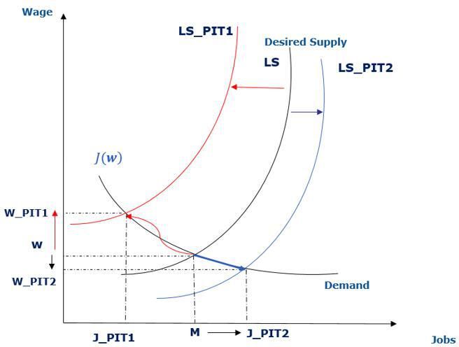
Another set of outcomes that the EUROLAB model can deliver is linked to changes in employment, inactivity and unemployment when taking into account the demand side of the labour market. Assuming an elasticity of labour demand of -0.5, the equilibrium model (Section 4) applies running an optimisation procedure to search the value of the change in average wage (parameter v, Section 4) that corresponds to a new labour market equilibrium status under the reform. The optimization procedure is explained in details in Narazani and Colombino (2021) The results are shown in Table A9.¹⁵ If equilibrium conditions are not taken into account, the PIT1 reform should shift the desired labour supply curve (Figure 1 LS_PIT1) to the left and reduce total employment by 0.66%. A new market equilibrium condition that requires consistency between the number of jobs available and the desired labour supply is achieved through a movement along the demand curve and an adjustment of the wage rate. Indeed, the equilibrium condition leads to a 1.24% increase in wages and a 0.62% decrease in employment, mainly offset by a 6% increase in inactivity rate and 5.5% in unemployment. The increase in unemployment is mainly due to the generosity of the unemployment benefit amounts which, unlike wage rates, were assumed unchanged in this exercise. It is important to stress that in the equilibrium model, only an employment equilibrium constraint is imposed for ease of computation and the imposition of an equilibrium constraint on unemployment can lead to different results. On the contrary, the reform PIT2 is expected to increase labour supply by 0.89% and shift the curve of labour supply (Figure 2, LS_PIT2) to the right. A new labour market equilibrium is achieved, with the wage rate falling by 1.69% and a lower increase in employment (0.85%).

Figure 2

Download asset Open asset

4.2 A EUROLAB application related to sectoral demand shocks

The multidimensional version of EUROLAB has been developed during the COVID-19 pandemic period, 2020-2021. Restrictive measures taken by EU countries to mitigate the spread of the virus led to the cessation of economic activity and severe job losses, in particular in the second quarter of 2020. The structure of labour market has undergone a dramatic change, characterized by a decline in employment and in the total number of hours worked, which has not been felt in the same way in all the sectors of activity. Some sectors of activity, such as non-essential services and production, have been more exposed to lockdown restrictions than others and have therefore experienced a greater reduction in working hours and employment. However, due to the delay in obtaining sufficient data, it is difficult to make a precise assessment of the extent of job losses and forecast of working hours for subsequent months or longer periods. In order to overcome the limitation of real-time data on employment, in particular at sectoral level, as well as the limitation of existing studies that consider exogenous transitions from work to unemployment or inactivity (or vice versa), we have built the multidimensional version of EUROLAB that takes into account differences between occupational sectors and employment statuses and allows for transitions to and from unemployment and inactivity status. Being capable to model the behavioural reactions of individuals within the labour market, depending on their occupational sector or employment status, the multidimensional version can be used to consider behavioural reactions to external sectoral demand shocks in employment.

Narazani and Colombino (2021), show how the multidimensional choice set of EUROLAB can be used to consider endogenous reactions to labour demand shocks as well as to assess the effectiveness of policy reforms, such as job retention schemes, in absorbing the impact of these shocks on employment under alternative hypothetical scenarios regarding the timing of reforms. In addition they show theoretically how the EUROLAB model can be used to assess the short-term and long-term effects of job retention policies and, in particular, to deliver differentiated results depending on whether the retention policy was implemented before or after the new labour market equilibrium was achieved. To illustrate the theoretical model, they perform a simulation of the effects of a hypothetical wage subsidy using the Italian module of EUROMOD as well as the Italian version of EU-SILC, the 2016 release, and show in particular how sectoral demand shocks lead to lower wages and employment and an increase in unemployment under equilibrium conditions. In order to assess the potential impact of a demand shock in the presence of a simplified wage subsidy scheme, they simulate an ex ante and ex post scenario that differ from each other in the timing of when the subsidy is allocated to potential beneficiaries – before or after labour market equilibrium is achieved. In the ex post scenario, the model predicts an increase in employment compared to the equilibrium situation in the absence of the wage subsidy, mainly due to the consideration of the recipients as employed. The ex ante scenario predicts a smaller increase in employment which would correspond to a long-term labour market equilibrium. These results imply that the timing of the introduction (or announcement) of the wage subsidy matters when determining the short and long-term impact of such policy.

4.3 Examples using a one-dimensional version of EUROLAB

The EUROLAB model needs to be considered from a holistic perspective, taking into account both the one-dimensional and multidimensional versions. Therefore, for the sake of completeness, this subsection discusses a set of examples where the one-dimensional version of EUROLAB that relies on a choice set consisting of working hours has been used. These examples regard fiscal reforms, mostly analysed within the framework of the European Semester or been put forward in policy debates.¹⁶ These reforms, either hypothetical or part of political debate, are designed with the objective of reducing the tax burden in particular on low-income individuals, reducing income inequality and/or increasing labour participation of under-employed segments of the population. Often they are constrained to be budget neutral and may represent a tax shift from labour to tax bases that are less detrimental to growth.

We exemplify the usefulness of a one-dimensional version of EUROLAB by presenting four main types of policy simulations.¹⁷ The first type regards changes in tax bracket, the second one involves tax shifting from labour to property, the third type considers changes in the amount of in-work tax credits, and the last type concerns changes in childcare-related subsidies for working mothers.

The first example regards the simulation of a hypothetical tax reform for Germany (European Commission, 2019), a country with a relatively high share of revenues from taxes on labour. The hypothetical reform is intended to flatten the “middle-class bulge”, a peculiarity of the German income tax regime generated by the sharp increase of the marginal tax rate (from 14% to 24%) in the 2nd tax bracket between EUR 8,653 to EUR 13,669. More specifically the reform consists in extending the upper threshold of this bracket to EUR 16,500. Simulation results indicate that after the reform, women are expected to increase their labour supply more than men, partly because they benefit more from the reform and partly because they have high part-time employment rates, which leaves space for adjustment in working hours. Furthermore, given relatively low levels of inactivity and unemployment in Germany, most labour supply response comes primarily from the intensive margin rather than the extensive margin. However, the highest responses come from women located in the first part of the income distribution due to a lower marginal effective tax rate paid after the reform and a higher labour supply elasticity that characterizes this population segment. The positive effects on labour are very limited for the top income deciles.

The second type of reform involves a hypothetical tax shift from labour to property in Italy (2020 European Semester Country Report – Italy).¹⁸ Italy is another EU country where the tax structure relies heavily on labour, with other tax bases being exploited less. In fact there is scope for exploiting more recurrent property taxes, more specifically those applied to main residences as they were abolished in 2014, leading to a substantial revenue loss. Moreover, although employment continued to increase in 2019, the Italian labour market was still characterized by high shares of involuntary unemployment and inactivity rates as well as underemployment especially among women and young people. In light of this tax structure, JRC simulated a tax shift from labour to property by (1) reintroducing taxes on all residences exempting or not low-value properties and eventually low-income pensioners, and (2) using the additional fiscal revenues to reduce the tax burden, namely, social security contributions paid by employees with an annual income below EUR 24,600. After the tax shift, the model predicted a rise in the labour force participation by 1.6% and total hours worked by 2.3% for women and 0.8% for men on average, with stronger responses for low-income workers who benefitted most from the tax shifting.

The third example regards an announced reform to the existing in-work tax credit scheme in Italy (European Commission, 2020), approved later that year in July 2020 by the Italian Parliament. The existing tax credit, targeting workers, amounted to EUR 80 per month for annual income between EUR 8,000 to 24,600, gradually phasing out for incomes of EUR 26,600 or more. The reform was announced to (1) increase the tax credit amount to EUR 100 per month for income up to EUR 28,000, (2) gradually reduce this amount to EUR 80 per month for annual income of EUR 35,000, and (3) phase out completely at EUR 40,000. After the reform, the model predicted (Box 4.1.1) an increase in participation rates by 2.3% for women and 0.9% for men, and total hours worked by 2.6% and 0.9% for women and men, respectively.

The fourth example of behavioural analysis regards a hypothetical reform on rationalising childcare benefits in Italy (European Commission, 2018). The reform was aimed at raising the low participation of mothers in the labour market. The reforms consisted in replacing four childcare-related bonuses (Voucher babysitting, Bonus bebè, Bonus mamma, Assegno di maternità), which seemed to not properly meet working mothers’ needs as well as overlapping in eligibility conditions, with a single in-work benefit, targeting low-income working mothers with children aged under three. The model predicted an increase in the labour market participation of around 17% and the average weekly working hours of around 20%. It is important to note that for this exercise, we adopted the methodological approach described in Figari and Narazani 2020 to account for the possible interaction between labour supply and childcare choices. For that purpose, the EUROLAB one-dimensional version was modified in order to address properly the labour supply patterns of specific population groups such as working mothers and specific benefit-related policies such as those related to childcare. More specifically, EUROLAB was enriched with information on childcare fees in public and private sectors in order to endogenously consider the childcare decisions of working mothers. This extension of EUROLAB was also important for assessing the impact of hypothetical reforms of decreasing childcare costs in four EU countries (ESDE report 2019) on labour supply of mothers and the usage of formal child care.¹⁹ The behavioural analysis pointed out that reducing childcare costs by half is expected to increase the use of formal childcare and the labour supply of mothers in countries where childcare costs are relatively high (Finland and the Netherlands). In countries with relatively low childcare cost (Hungary and Lithuania) the increase in formal childcare use is very small, suggesting that policies focused on increasing availability might work better.

5. Future extensions of EUROLAB

The multidimensional modelling of EUROLAB offers several functionalities that can be exploited to extend the model in several directions. This section describes potential extensions of EUROLAB synergies with in-home EUROMOD functionalities such as the Indirect Tax Tool – version 3 (IITv3), the EUROMOD WEALTH Taxation Tool (EWIGE) and the Labour Market Transition tool (LMA).

5.1 Indirect taxes

Reforms on indirect taxation can trigger behavioural effects on the labour supply decisions of households that cannot be captured by EUROMOD or similar non-behavioural microsimulation models. This is also the case with the current version of EUROLAB. For example, increases in VAT, reduced or standard rates have been frequently discussed in EU countries, for example, as part of fiscal consolidation packages taken in prior to the global financial crisis. Such reforms can stand alone or be part of budget-neutral tax-shifting from personal income tax or social security contributions for the whole population or for a part of it that can loose from VAT increase. However, simulations of indirect tax changes cannot be performed using EUROMOD as the SILC data, the underlying data of EUROMOD, do not contain detailed information on household expenditures. For that purpose, data from the Household Budget Survey are used together with the SILC data to develop an extension of the EUROMOD tool IITv3 that allows running reforms on indirect taxes at a highly disaggregated level of consumption.²⁰ Therefore a potential extension of the EUROLAB model can be towards the behavioural effects of indirect tax reforms or policy mixes between direct and indirect tax tools. In light of this extension, linking EUROLAB with the EUROMOD ITTv3 tool can help in assessing the behavioural effects of potential policy mixes of direct and indirect taxes. The linking mechanism can enable the simultaneously generation of household disposable income (through EUROMOD) and household expenditures in durable and nondurable goods at each counterfactual choice of labour supply.

5.2 Wealth taxation

Announcements of changes in wealth taxation parameters can result in labour supply reactions of the potential heirs. For example, decreasing the inheritance tax exemption threshold or increasing the tax rate leads to a lower income from inheritance and therefore a lower dependency on inheritance income which in turn may increase the labour supply of heirs if leisure is a normal good. Therefore, accounting for the labour effects of inheritance tax reforms might be important for assessing net budgetary effects after the reform. EWIGE 2 (Boone et al., 2019) represents the EUROMOD Wealth taxation tool that allows the simulation of wealth-related taxes and fiscal policies often deemed as an optimal tool for reducing inequality. It integrates the Household Finance and Consumption Survey (HFCS) data in EUROMOD, enabling assessment of the distributional effects of different current and hypothetical wealth taxes and policies. Yet, behavioural effects of wealth-related tax reforms are not taken into account by the EWIGE 2. For that purpose, EUROLAB can be linked with EWIGE and help quantify the second and third-round effects on heirs. The synergy of these models becomes even more important in face of potential tax shifting reforms from labour to wealth.

5.3 Labour Market Adjustment (LMA)

Constructing the unemployment alternative and simulating respective unemployment benefits in the EUROLAB model require a set of assumptions on eligibility criteria and calculation of the wage rate. These assumptions may differ country-by-country and setting them manually in EUROLAB may cause computational errors that in turn lead to an over/underestimation of unemployment benefits. Such a potential source of bias can be circumvented through a EUROMOD tool, namely the LMA Add-on, which allows changes in the labour market status of an individual or simulation of hypothetical labour market scenarios.²¹ More concretely, the LMA Add-on can be used to construct the unemployment alternative and simulate corresponding benefits in line with the country-specific rules through its capacity of simulating the transition from employment to unemployment, either short-term or long-term. In addition, EUROLAB can benefit from the additional features of the LMA Add-on to relax the assumption of annual transitions to unemployment (or employment) by allowing users to set-up the duration of transitions.

Recently, the LMA Add-on has been enhanced with the intention of simulating the effect of monetary compensation schemes, widely used in EU countries to cushion the income loss of employed and self-employed households from the COVID-19 crisis. The enhancement consists in simulating labour market transitions from work to either unemployment or monetary compensations schemes through the LMA Add-on in order to simulate with EUROMOD the budgetary and distributional impact of these schemes. The LMA Add-on can be linked with EUROLAB to assess behavioural responses triggered by these schemes or similar policy interventions in a medium and long-run perspective using the labour demand module of EUROLAB (chapter 4). A simplistic representation of these monetary schemes is implemented in Narazani and Colombino (2021) but, as the authors argue, actual policies and more recent statistics are needed in order to analyse the extent to which the existence and design of such schemes matters in order to strengthen the resilience of labour markets to economic shocks.

6. Conclusions

The EU-wide microsimulation model, EUROMOD, is a static model that does not account for behavioural responses when assessing policy effects. However, its ability to replicate closely existing and counterfactual fiscal reforms together with the heterogeneity of the underlying data represent an appropriate tool to build a behavioural microsimulation model that can be used to assess the impact of fiscal or economic policies on labour supply and overall employment in EU countries. This paper provides an overview of EUROLAB, the EU labour supply-demand microsimulation model build on EUROMOD, that similarly to other behavioural microsimulation models, estimates a set of structural parameters of utility function and applies them to predict labour supply responses to hypothetical or real policy reforms. However, unlike other behavioural models, EUROLAB adopts a multidimensional approach in the construction of choice setting as well as including a representation of both labour supply and demand accounting in this way for labour market equilibrium achieved through wage adjustment.

After describing the modelling of the multidimensional structure of the choice set and the labour supply-demand mechanism, the paper discusses the potential use of the model and possible extensions through synergies with in-home EUROMOD functionalities such as the Indirect Tax Tool, the EUROMOD WEALTH Taxation Tool and the Labour Market Transition Add-on. For example, a potential synergy between EUROLAB and the Indirect Tax EUROMOD extension can help in assessing behavioural effects of indirect tax reforms like increases in VAT rates for specific goods or even more ambitious reforms like those on green taxation. On the other hand, a potential synergy with the EUROMOD Wealth extension can help in assessing the effects of announced changes in wealth taxation parameters on labour supply of potential heirs, which in turn might be important for assessing the net budgetary effects of the reform. Furthermore, a synergy of EUROLAB with the Labour Market Transition tool, a functionality of EUROMOD that allows changes in the labour market status, can help in automatizing the construction of unemployment alternatives in EUROLAB and the simulation of corresponding benefits in line with the country specific rules through its capacity to simulate the transition from employment to unemployment, either short-term or long-term. In addition, linking the LMA Add-on with EUROLAB can help in assessing behavioural responses triggered by monetary compensation schemes or similar policy interventions in a medium and long-run perspective using the labour demand module of EUROLAB.

EUROLAB proves to be relevant for assessing the effects of policies implemented by Member States in order to mitigate the negative effects of the Covid-19 pandemic on employment. However, its use may go beyond COVID and post-COVID analysis. For example, EUROLAB can be used to predict the aggregated behavioural effects of future changes in the working-age population that are related to internal or external migration flows, ageing of specific population groups or educational composition. For that, data on population projections can be integrated in the micro-data using, for example, a reweighting approach and modifying the individuals’ sampling weights in order for them to correspond to the projected working-age population in a given year. On the other hand, another use of EUROLAB can be towards gender-biased reforms, for example, to assess the behavioural effects of changes in the Barcelona targets that ensure suitable childcare provision as an essential step towards equal opportunities in employment between women and men. In this case, a more advanced modelling approach that can embed childcare preferences and childcare rationing constraints in a labour supply-demand setting would be the appropriate tool rather that a reweighting approach as in the former example.

Optimal taxation is another domain where EUROLAB can provide valuable assistance for policy analysis in the EU area. Assessing quantitatively the optimal system of taxation in order to achieve a desired target of income distribution with the least inefficiency is an important objective of the European Commission. EUROLAB can help in this debate by providing empirical analysis that enhances understanding. For that, first we have to choose a criterion that establishes the optimality of a given policy reform. For example, inefficiency reduction may represent a policy-relevant criterion in case of a minimum income scheme reform targeted to reduce poverty, while targeting inequality reduction might be more appropriate when assessing labour incentive reforms such as in-work tax credits. A combination of both of these evaluation criteria through a social welfare function may provide a more conclusive result in the identification of the optimal reform that targets simultaneously efficiency and equality objectives.

Footnotes

1.

For example, an across a board increase in property tax is supposed to increase the tax burden of low-income individuals and trigger changes in their labour behaviour. Similarly, a change in mortgage tax relief may alter labour supply behaviour

2.

Fiscal reforms can trigger behavioural effects not only on labour markets but also on consumption, wealth and capital investment, educational choices or childcare services or services for the elderly. All these behavioural effects are not considered in EUROMOD.

3.

For example, individuals may have a strong preference for working in the public sector. This preference may often be so strong that it can direct them into inactivity and educational training.

4.

As Boer argues, this insignificant effect on behavioural responses is possibly due to the small share of individuals in involuntary unemployment in the Netherlands.

5.

Institute for Social and Economic Research, University of Essex and Joint Research Centre, European Commission, EUROMOD: Version I3.0+ [software], January 2021. The EUROMOD model is maintained and updated by the European Commission Joint Research Centre, for further information see https://euromod-web.jrc.ec.europa.eu/ and Sutherland and Figari (2013).

6.

For example, the survey year for the EU-SILC 2018 wave is 2018, while the income reference period is 2017.

7.

Furthermore, the time lag may cause a loss in data quality, especially when the date of interview is far removed from the reference income period, especially for individuals in unstable employment.

8.

We consider the wage rates as exogenous, although they can be treated as endogenous by estimating wage functions simultaneously with the utility function parameters and the job opportunity density, all embedded in the maximum likelihood function

9.

The details of this approach are given in appendix D of Dagsvik and Strøm (2004).

10.

The first method is implemented estimating sequentially the selection equation and the wage equation in STATA. The other two methods are implemented using the selmlog command written by Bourguignon et al. (2007).

11.

The estimates of the wage equation are available upon request from the author.

12.

The next version of EUROLAB will allow the user to change the parameter of labour demand elasticity in the EUROLAB interface.

13.

The survey is representative for the national population at the regional level, and is the national component of the EU-SILC carried out annually to collect comparable information on income, poverty, social exclusion and living conditions across EU countries.

14.

Low-income household means a family whose members living together have an equivalised disposable income that is part of the lowest income quintile. On the contrary, high-income household means a family whose members living together have an equivalised disposable income that is part of the highest income quintile.

15.

We use the Amoeba, an optimisation routine written in STATA. Amoeba is an efficient (derivative-free) algorithm for optimising a multidimensional function developed by Nelder and Mead. Convergence rules are needed to break the iteration cycle. We set a step size (percentage change in each parameter used to set up Amoeba in the parameter space) equal to 0.1 and a tolerance (the tightness of Amoeba before the algorithm quits) equal to E-06.

16.

The European Semester is a cycle of economic and fiscal policy coordination within the EU. It is part of the European Union's economic governance framework. Its focus is on the 6-month period from the beginning of each year, hence its name – the 'Semester'.

17.

Christl et al., 2019 make use of the unilateral version of EUROLAB to analyse labour supply responses to changes in social assistance. Similarly, Christl and De Poli, 2021 assess behavioural effects of implementing a child tax credit in Austria in 2019

18.

See Box 4.1.1: EUROMOD-QUEST simulation – Shifting taxes from labour to property in Italy.

19.

See Annex 2: Euromod simulations of the impact of the reduction of childcare costs on the use of the service and on the mothers’ labour supply decisions, Employment and Social Developments Review, 2019.

20.

For more details on ITTv3, see Akoğuz et al. (2020).

21.

For more details, see Poli et al. (2021).

Appendix A

A.1. Conditional Logit results

Table A1

Conditional Logit results

	Couples	Single Women	Single Men
clogit dependent variable
In-work dummy Male	-1.069^* (-2.51)		-0.0994 (-0.39)
Part-time dummy - Male	-2.935^*** (-8.65)		-2.255^*** (-9.94)
Full-time dummy - Male	-0.0331 (-0.16)		0.633^*** (3.33)
Over-time dummy - Male	0.877^*** (3.92)		1.637^*** (7.66)
In-work dummy Female	0.537^** (2.62)	0.329 (1.33)
Part-time dummy - Female	-1.188^*** (-11.33)	-0.953^*** (-5.74)
Full-time dummy - Female	0.681^*** (5.62)	1.447^*** (8.01)
Over-time dummy - Female	0.364^* (2.45)	1.366^*** (6.65)
Leisure - Male	0.0866 (1.42)		0.0250 (0.80)
Leisure square - Male	-0.000653 (-1.85)		0.000415 (1.69)
Leisure x age - Male	-0.00477^* (-2.23)		-0.00286^** (-3.03)
Leisure x age square - Male	0.0000631^** (2.81)		0.0000359^** (3.27)
Leisure x #children - Male	-0.00575^* (-1.98)		0.00407 (0.66)
Leisure x #children < 3 year - Male	-0.00197 (-0.22)		-0.0151 (-0.22)
Leisure x #children 3-6 year - Male	-0.000181 (-0.02)		-0.0183 (-0.45)
Leisure x Migrant - Male	-0.0150 (-1.70)		-0.0247^*** (-4.78)
Leisure x Mortgage - Male	-0.000614^* (-2.20)		-0.000482 (-1.44)
Leisure - Female	0.123^** (2.93)	0.00382 (0.11)
Leisure square - Female	-0.000759^*** (-3.45)	0.00117^*** (4.54)
Leisure x age - Female	-0.00127 (-0.80)	-0.00550^*** (-4.91)
Leisure x age square - Female	0.0000133 (0.73)	0.0000671^*** (5.26)
Leisure x #children - Female	0.00464^* (2.33)	0.0118^*** (3.65)
Leisure x #children < 3 year - Female	0.00702 (1.40)	0.0148 (1.62)
Leisure x #children 3-6 year - Female	0.00108 (0.26)	0.00789 (0.92)
Leisure x Migrant - Female	-0.0121^* (-2.02)	-0.0278^*** (-5.68)
Leisure x Mortgage - Female	-0.000177 (-1.06)	-0.000427 (-1.30)
Leisure Male x Leisure Female	0.000768^*** (5.14)
Net income	0.0109^*** (13.44)	0.00794^*** (10.66)	0.00542^*** (9.54)
Net income square	-0.00000277^*** (-16.92)	-0.00000271^*** (-7.37)	-0.00000198^*** (-8.51)
Net income x household size	0.000256 (1.93)	0.000463 (1.86)	0.000783^*** (3.89)
Net income x Leisure - Male	-0.0000234^** (-3.26)		0.00000576 (1.05)
Net income x Leisure - Female	-0.0000389^*** (-7.36)	0.00000760 (1.13)
Observations	217216	24024	26168
ll	-10420.5	-4878.9	-4924.8
r2_p	0.262	0.219	0.276
aic	20904.9	9791.7	9883.6
bic	21234.2	9929.2	10022.5

t statistics in parentheses.
*p < 0.05, ^** p < 0.01, ^*** p < 0.001.

A.2. Prediction results

Table A2

The average value of predicted probabilities and observed fractions across labour supply alternatives

	Predicted	Observed
A. Women in Couple
Inactive	0.017755	0.020625
Unemployed	0.027174	0.022982
5 - 22	0.011039	0.00442
22 - 39	0.195358	0.2033
39 - 56	0.748674	0.748674
B. Men in Couple
Inactive	0.041128	0.043017
Unemployed	0.059956	0.047731
5 - 22	0.082874	0.070418
22 - 39	0.470726	0.493518
39 - 56	0.345315	0.345315
C. Single Men
Inactive	0.233291	0.231268
Unemployed	0.159889	0.162575
5 - 22	0.191616	0.188676
22 - 39	0.213798	0.218327
39 - 56	0.315418	0.316016
D. Single Women
Inactive	0.235618	0.235188
Unemployed	0.195866	0.199835
5 - 22	0.194552	0.19799
22 - 39	0.252569	0.254291
39 - 56	0.310901	0.305658

A.3. Elasticities results

Table A3

Labour elasticities for All, it

		All			Couples			Singles
		Total	Extensive	Intensive	Total	Extensive	Intensive	Total	Extensive	Intensive
Education	Low level	0.137	0.109	0.028	0.106	0.083	0.024	0.174	0.142	0.033
	Middle level	0.119	0.093	0.026	0.090	0.065	0.024	0.156	0.127	0.029
	High level	0.088	0.058	0.029	0.073	0.040	0.033	0.107	0.083	0.024
Age	20-30	0.175	0.134	0.041	0.147	0.100	0.047	0.185	0.147	0.038
	31-40	0.112	0.085	0.027	0.097	0.071	0.027	0.131	0.103	0.028
	41-on	0.112	0.086	0.026	0.084	0.059	0.025	0.151	0.124	0.028
Child	Yes	0.132	0.102	0.031	0.101	0.070	0.031	0.148	0.117	0.030
	No	0.097	0.073	0.023	0.085	0.061	0.024	0.164	0.142	0.022
Migrant	Yes	0.118	0.091	0.026	0.089	0.063	0.026	0.156	0.128	0.027
	No	0.108	0.072	0.036	0.105	0.075	0.030	0.111	0.068	0.043
Income level	Low	0.166	0.131	0.036	0.132	0.103	0.030	0.208	0.165	0.043
	Middle	0.100	0.083	0.018	0.071	0.057	0.015	0.142	0.120	0.022
	High	0.050	0.019	0.031	0.045	-0.001	0.046	0.056	0.041	0.015
Total		0.117	0.089	0.027	0.090	0.064	0.026	0.150	0.121	0.029

Table A4

Labour elasticities, men

		All			Couples			Singles
		Total	Extensive	Intensive	Total	Extensive	Intensive	Total	Extensive	Intensive
Education	Low level	0.127	0.103	0.025	0.076	0.064	0.012	0.186	0.147	0.039
	Middle level	0.104	0.082	0.023	0.053	0.038	0.014	0.164	0.131	0.033
	High level	0.074	0.038	0.036	0.056	0.014	0.041	0.099	0.071	0.028
Age	20-30	0.175	0.130	0.045	0.085	0.050	0.034	0.191	0.144	0.047
	31-40	0.095	0.072	0.023	0.047	0.035	0.013	0.141	0.109	0.033
	41-on	0.101	0.076	0.025	0.064	0.043	0.021	0.158	0.127	0.031
Child	Yes	0.139	0.106	0.033	0.091	0.063	0.029	0.159	0.124	0.035
	No	0.051	0.036	0.015	0.046	0.031	0.015	0.147	0.135	0.012
Migrant	Yes	0.107	0.082	0.025	0.061	0.041	0.020	0.163	0.132	0.031
	No	0.096	0.057	0.039	0.058	0.041	0.018	0.129	0.072	0.058
Income level	Low	0.153	0.117	0.037	0.083	0.068	0.015	0.240	0.177	0.063
	Middle	0.081	0.079	0.002	0.030	0.040	-0.010	0.147	0.130	0.017
	High	0.066	0.013	0.054	0.084	-0.012	0.097	0.050	0.035	0.015
Total		0.106	0.080	0.026	0.061	0.041	0.020	0.159	0.125	0.034

Table A5

Labour elasticities, women

		All			Couples			Singles
		Total	Extensive	Intensive	Total	Extensive	Intensive	Total	Extensive	Intensive
Education	Low level	0.150	0.118	0.032	0.146	0.107	0.039	0.157	0.134	0.023
	Middle level	0.135	0.105	0.030	0.126	0.092	0.034	0.148	0.123	0.025
	High level	0.098	0.074	0.024	0.087	0.061	0.026	0.114	0.092	0.022
Age	20-30	0.174	0.139	0.035	0.172	0.120	0.052	0.176	0.153	0.022
	31-40	0.129	0.098	0.031	0.137	0.099	0.038	0.116	0.095	0.021
	41-on	0.123	0.096	0.027	0.107	0.078	0.029	0.144	0.120	0.024
Child	Yes	0.123	0.095	0.028	0.111	0.076	0.034	0.130	0.107	0.023
	No	0.134	0.103	0.030	0.124	0.092	0.032	0.167	0.144	0.024
Migrant	Yes	0.129	0.101	0.028	0.117	0.085	0.032	0.147	0.124	0.023
	No	0.120	0.085	0.034	0.144	0.103	0.041	0.092	0.065	0.027
Income level	Low	0.179	0.144	0.035	0.182	0.137	0.044	0.176	0.153	0.023
	Middle	0.122	0.087	0.035	0.112	0.073	0.039	0.137	0.108	0.028
	High	0.031	0.027	0.004	0.005	0.010	-0.006	0.065	0.049	0.016
Total		0.128	0.099	0.029	0.120	0.087	0.033	0.140	0.117	0.023

Appendix B

B.1. Pure Labour supply effects

Table A6

Labour supply changes by gender and household type, employees

		Baseline, 2021	% Change after PIT1	% Change after PIT2
Hours of work
Men	In couple - with children	39.14	-0.31%	0.29%
	In couple - without children	37.63	-0.50%	0.63%
	Single - with children	35.67	-0.95%	1.88%
	Single - without children	34.68	-0.75%	1.59%
Women	In couple - with children	30.88	-1.05%	1.47%
	In couple - without children	31.61	-0.97%	1.64%
	Single - with children	31.71	-1.08%	2.51%
	Single - without children	33.16	-0.87%	1.84%
Participation
Men	In couple - with children	0.97	-0.29%	0.31%
	In couple - without children	0.94	-0.47%	0.61%
	Single - with children	0.90	-0.85%	1.46%
	Single - without children	0.88	-0.69%	1.31%
Women	In couple - with children	0.90	-0.70%	0.81%
	In couple - without children	0.92	-0.64%	0.87%
	Single - with children	0.86	-0.94%	1.63%
	Single - without children	0.89	-0.75%	1.23%
Unemployment
Men	In couple - with children	0.02	9.39%	-11.37%
	In couple - without children	0.04	6.75%	-11.39%
	Single - with children	0.05	7.74%	-14.01%
	Single - without children	0.06	3.95%	-10.22%
Women	In couple - with children	0.05	6.75%	-9.00%
	In couple - without children	0.05	6.52%	-10.69%
	Single - with children	0.07	6.01%	-12.03%
	Single - without children	0.06	4.70%	-10.57%
Inactivity
Men	In couple - with children	0.01	9.49%	-7.48%
	In couple - without children	0.02	7.95%	-6.44%
	Single - with children	0.05	7.07%	-11.48%
	Single - without children	0.06	6.35%	-9.05%
Women	In couple - with children	0.04	6.49%	-6.13%
	In couple - without children	0.04	7.42%	-7.97%
	Single - with children	0.07	5.90%	-8.71%
	Single - without children	0.06	6.99%	-8.74%

Note: Children are defined as son-daughter of the decision-making unit. They are not older than 18 years, or if older, in education.

Table A7

Labour supply changes by gender and household type, self-employed

		Baseline, 2021	% Change after PIT1	% Change after PIT2
Hours of work
Men	In couple - with children	41.87	-0.28%	0.25%
	In couple - without children	39.32	-0.44%	-0.10%
	Single - with children	37.09	-1.04%	2.63%
	Single - without children	37.33	-0.77%	1.38%
Women	In couple - with children	32.76	-0.85%	1.23%
	In couple - without children	32.73	-0.85%	1.17%
	Single - with children	34.19	-1.09%	2.02%
	Single - without children	34.78	-0.70%	1.21%
Participation
Men	In couple - with children	0.97	-0.25%	0.12%
	In couple - without children	0.94	-0.40%	-0.11%
	Single - with children	0.89	-0.95%	1.53%
	Single - without children	0.90	-0.71%	1.01%
Women	In couple - with children	0.93	-0.57%	0.52%
	In couple - without children	0.93	-0.55%	0.46%
	Single - with children	0.90	-0.81%	0.78%
	Single - without children	0.90	-0.66%	0.69%
Unemployment
Men	In couple - with children	0.01	8.37%	-3.83%
	In couple - without children	0.03	5.56%	3.09%
	Single - with children	0.05	8.28%	-12.55%
	Single - without children	0.04	6.21%	-8.81%
Women	In couple - with children	0.03	7.64%	-6.55%
	In couple - without children	0.03	7.20%	-5.24%
	Single - with children	0.04	6.75%	-6.52%
	Single - without children	0.04	5.85%	-6.19%
Inactivity
Men	In couple - with children	0.01	9.05%	-4.93%
	In couple - without children	0.03	6.31%	0.10%
	Single - with children	0.06	7.72%	-12.98%
	Single - without children	0.06	6.29%	-9.04%
Women	In couple - with children	0.04	7.99%	-7.61%
	In couple - without children	0.04	7.66%	-7.08%
	Single - with children	0.07	7.07%	-6.83%
	Single - without children	0.06	5.95%	-6.07%

Note: Children are defined as son-daughter of the decision-making unit. They are not older than 18 years, or if older, in education.

Appendix C

Table A8

Labour supply changes by gender and income quintiles

		Baseline, 2021	% Change after PIT1	% Change after PIT2
Hours of work
Men	I-II	34.42	-1.07%	1.47%
	III-IV	36.85	-0.98%	1.78%
	V-VI	37.40	-0.71%	1.47%
	VII-VIII	37.76	-0.43%	1.13%
	IX-X	38.75	0.05%	-0.97%
Women	I-II	28.18	-1.75%	2.12%
	III-IV	31.89	-1.78%	3.32%
	V-VI	33.08	-1.24%	2.58%
	VII-VIII	35.19	-0.57%	1.99%
	IX-X	34.74	0.34%	-0.45%
Participation
Men	I-II	0.87	-0.89%	1.11%
	III-IV	0.91	-0.84%	1.36%
	V-VI	0.93	-0.64%	1.16%
	VII-VIII	0.94	-0.44%	0.94%
	IX-X	0.94	-0.05%	-0.58%
Women	I-II	0.78	-1.29%	1.44%
	III-IV	0.86	-1.36%	2.14%
	V-VI	0.89	-0.99%	1.72%
	VII-VIII	0.93	-0.57%	1.30%
	IX-X	0.91	0.01%	-0.47%

B.2. Labour supply effects accounting for demand side of labour market

Table A9

% Changes in employment, unemployment and inactivity rate after the PIT reforms

	Baseline	PIT1		PIT2
	Baseline	No Equilibrium (%)	With Equilibrium (%)	No Equilibrium (%)	With Equilibrium (%)
Employment	15854397	-0.66%	-0.62%	0.89%	0.85%
Inactivity	916796	6.49%	6.03%	-7.49%	-7.05%
Unemployment	762628	5.83%	5.54%	-9.50%	-9.29%
Wages			1.24%		-1.69%

*Definitions: Employment = Total number of people in employment, only labour supply endogenous sample, Inactivity = Total number of people in inactivity, only behavioural sample, Unemployment = Total number of people in unemployment, only behavioural sample, v = Parameter of percentage change in wages.

References

1
Accounting for family background when designing optimal income taxes: a microeconometric simulation analysis
1. R Aaberge
2. U Colombino
(2012)
Journal of Population Economics 25:741–761.
https://doi.org/10.1007/s00148-010-0331-y
- Google Scholar
2
Population Ageing, Social Security and Taxation: Modelling Our Future
et al. (2007)
Population Ageing and Fiscal Sustainability: An Integrated Micro-Macro Analysis of Required Tax Changes, Population Ageing, Social Security and Taxation: Modelling Our Future, Emerald Group Pub.
- Google Scholar
3
Labour supply in Italy: an empirical analysis of joint household decisions, with taxes and quantity constraints
(1999)
Journal of Applied Econometrics 14:403–422.
https://doi.org/10.1002/(SICI)1099-1255(199907/08)14:4<403::AID-JAE520>3.0.CO;2-4
- Google Scholar
4
EVALUATING ALTERNATIVE REPRESENTATIONS OF THE CHOICE SETS IN MODELS OF LABOR SUPPLY
(2009)
Journal of Economic Surveys 23:586–612.
https://doi.org/10.1111/j.1467-6419.2008.00573.x
- Google Scholar
5
Labor Supply Responses and Welfare Effects of Tax Reforms
1. R Aaberge
2. JK Dagsvik
3. S Strøm
4. S Strom
(1995)
The Scandinavian Journal of Economics 97:635–659.
https://doi.org/10.2307/3440547
- Google Scholar
6
“A New Indirect Tax Tool for EUROMOD.”
1. E Akoğuz
2. B Capéau
3. A Decoster
4. L Sadeleer
5. D Güner
6. K Manios
7. AT Vanheukelom
(2020)
JRC Project no. JRC/SVQ/2018/B.2/0021/OC.
- Google Scholar
7
“Making work pay” in a rationed labor market
1. O Bargain
2. M Caliendo
3. P Haan
4. K Orsini
(2010)
Journal of Population Economics 23:323–351.
https://doi.org/10.1007/s00148-008-0220-9
- Google Scholar
8
Dynamic scoring of tax reforms in the european union
1. S Barrios
2. M Dolls
3. A Maftei
4. A Peichl
5. S Riscado
6. J Varga
7. C Wittneben
(2019)
Journal of Policy Analysis and Management 38:239–262.
https://doi.org/10.1002/pam.22105
- Google Scholar
9
Handbook of Econometrics
(2007)
Labor Supply Models: Unobserved Heterogeneity, Nonparticipation and Dynamics, Handbook of Econometrics, 1st, ed, Elsevier.
- Google Scholar
10
Employment, Hours of Work and the Optimal Taxation of Low-Income Families
1. R Blundell
2. A Shephard
(2012)
Review of Economic Studies, Oxford University Press.
- Google Scholar
11
Solo Self-Employment and Alternative Work Arrangements: A Cross-Country Perspective on the Changing Composition of Jobs
(2020)
Journal of Economic Perspectives 34:170–195.
https://doi.org/10.1257/jep.34.1.170
- Google Scholar
12
EWIGE 2 – Update and Extension of the EUROMOD Wealth Taxation Project No.JRC117204
1. J Boone
2. J Derboven
3. F Figari
4. S Kuypers
5. G Verbist
(2019)
Seville: European Commission, Joint Research Centre.
- Google Scholar
13
Selection Bias Corrections Based on the Multinomial Logit Model: Monte-Carlo Comparisons
(2007)
Journal of Economic Surveys 21:174–205.
https://doi.org/10.1111/j.1467-6419.2007.00503.x
- Google Scholar
14
Income and Living Conditions in Europe
(2010)
The distribution of employees’ labour earnings in the European Union: Data, concepts and first results, Income and Living Conditions in Europe, Luxembourg, Eurostat Statistical Books, Publications Office of the European Union.
- Google Scholar
15
Trapped in inactivity? Social assistance and labour supply in Austria
1. M Christl
2. S De Poli
(2021)
Empirica 48:661–696.
https://doi.org/10.1007/s10663-021-09507-8
- Google Scholar
16
Reducing the income tax burden for households with children: An assessment of the child tax credit reform in Austria No. JRC092019
(2019)
Seville: European Commission, Joint Research Centre.
- Google Scholar
17
Shifting taxes away from labour enhances equity and fiscal efficiency
(2020)
Journal of Policy Modeling 42:367–384.
https://doi.org/10.1016/j.jpolmod.2019.07.002
- Google Scholar
18
A new equilibrium simulation procedure with discrete choice models
1. U Colombino
(2013)
International Journal of Microsimulation 6:25–49.
https://doi.org/10.34196/ijm.00087
- Google Scholar
19
Alternative Basic Income Mechanisms: An Evaluation Exercise With a Microeconometric Model
(2010)
Basic Income Studies 5:Article 3.
https://doi.org/10.2202/1932-0183.1162
- Google Scholar
20
Designing a Universal Income Support Mechanism for Italy: An Exploratory Tour
1. U Colombino
2. E Narazani
(2013)
Basic Income Studies 8:1–17.
https://doi.org/10.1515/bis-2012-0010
- Google Scholar
21
Linking CGE and Microsimulation Models: A Comparison Different Approaches
1. G Colombo
(2018)
International Journal of Microsimulation 3:72–91.
https://doi.org/10.34196/ijm.00026
- Google Scholar
22
Aggregating Labour Supply and Feedback Effects in Microsimulation
1. J Creedy
2. A Duncan
(2005)
Australian Journal of Labour Economics 8:277–290.
- Google Scholar
23
Microsimulation Modelling of Taxation and The Labour Market: The Melbourne Institute Tax and Transfer Simulator
(2022)
Cheltenham: Edward Elgar.
- Google Scholar
24
Sectoral Labour Supply, Choice Restrictions and Functional Form
1. J Dagsvik
2. S Strøm
(2004)
Discussion Papers No. 388, September 2004 Statistics Norway, Research Department.
- Google Scholar
25
Willing to Pay for Security: A Discrete Choice Experiment to Analyse Labour Supply Preferences
1. Datta
(2019)
CEP Discussion Papers dp1632.
- Google Scholar
26
A Structural Analysis of Labour Supply and Involuntary Unemployment in the Netherlands
1. H-W de Boer
(2018)
De Economist 166:285–308.
https://doi.org/10.1007/s10645-018-9326-y
- Google Scholar
27
An Econometric Analysis of Residential Electric Appliance Holdings and Consumption
1. JA Dubin
2. DL McFadden
(1984)
Econometrica 52:345.
https://doi.org/10.2307/1911493
- Google Scholar
28
Sustainable growth for all: choices for the future of Social Europe
1. Employment and Social Developments Review
(2019)
29
SWEtaxben: A Swedish Tax/Benefit Micro Simulation Model and an Evaluation of A Swedish Tax Reform
(2009)
SSRN Electronic Journal 346:1391758.
https://doi.org/10.2139/ssrn.1391758
- Google Scholar
30
Commission Staff Working Document Country Report Italy 2018 Including an In-Depth Review on the prevention and correction of macroeconomic imbalances
1. European Commission
(2018)
31
Commission Staff Working Document Country Report Germany 2019 Including an In-Depth Review on the prevention and correction of macroeconomic imbalances
1. European Commission
(2019)
32
Commission Staff Working Document Country Report Italy 2020 Including an In-Depth Review on the prevention and correction of macroeconomic imbalances
1. European Commission
(2020)
33
The joint decision of female labour supply and childcare in Italy under costs and availability constraints
1. F Figari
2. E Narazani
(2020)
Economia Politica 37:411–439.
https://doi.org/10.1007/s40888-019-00160-w
- Google Scholar
34
Female Labor Supply
1. G Hanoch
(1980)
249–326, A Multivariate Model of Labor Supply: Methodology and Estimation, Female Labor Supply, Princeton University Press. Princeton, p.
- Google Scholar
35
Sample Selection Bias as A Specification Error
1. JJ Heckman
(1979)
Econometrica 47:153.
https://doi.org/10.2307/1912352
- Google Scholar
36
MICSIM - A behavioural microsimulation model for the analysis of tax-benefit reform in the Netherlands
1. E Jongen
2. H Boer
3. P Dekker
(2014)
CPB Background Document, https://www.cpb.nl/sites/default/files/publicaties/download/cpb-background-document-27nov2014-micsim.pdf, Accessed, 27 November 2014.
- Google Scholar
37
Labour Supply and Welfare Participation in Australian Two-Adult Households: Accounting for Involuntary Unemployment and the “Cost” of Part-time Work
1. GR Kalb
(2000)
Centre of Policy Studies/IMPACT Centre Working Papers bp-35.
- Google Scholar
38
Working Paper Series
1. A Klevmarken
(1997)
31, Behavioral Modeling in Micro Simulation Models. A Survey, Working Paper Series, Vol, 1997, Uppsala University, Department of Economics, p.
- Google Scholar
39
Dynamic scoring: A back-of-the-envelope guide
1. NG Mankiw
2. M Weinzierl
(2006)
Journal of Public Economics 90:1415–1433.
https://doi.org/10.1016/j.jpubeco.2005.11.006
- Google Scholar
40
Frontiers in Econometric
1. D McFadden
(1974)
105–142, Conditional Logit Analysis of Qualitative Choice Behavior, Frontiers in Econometric, New York, Academic Press, p.
- Google Scholar
41
Estimation of wage equations for New Zealand Working Paper 14/09
1. J Mercante
2. P Mok
(2014a)
Wellington: New Zealand Treasury.
- Google Scholar
42
Estimation of labour supply in New Zealand Working Paper 14/08
1. J Mercante
2. P Mok
(2014b)
Wellington: New Zealand Treasury.
- Google Scholar
43
Modelling sector-specific employment shocks with EUROLAB, a multi-dimensional behavioural model No. JRC12559
1. E Narazani
2. U Colombino
(2021)
Seville: European Commission.
- Google Scholar
44
FiFoSiM - An Integrated Tax Benefit Microsimulation and CGE Model for Germany
1. A Peichl
2. T Schaefer
(2009)
International Journal of Microsimulation 2:1–15.
https://doi.org/10.34196/ijm.00008
- Google Scholar
45
Documentation IZAψMOD: The IZA Policy Simulation Model
(2010)
IZA Discussion Paper No. 4865.
- Google Scholar
46
Accounting for labor demand effects in structural labor supply models
1. A Peichl
2. S Siegloch
(2012)
Labour Economics 19:129–138.
https://doi.org/10.1016/j.labeco.2011.09.007
- Google Scholar
47
Summary note for EUROMOD labour market adjustment add-on
1. SD Poli
2. T Hufkens
3. C Leventi
4. A Papini
(2021)
48
EUROMOD: the European Union tax-benefit microsimulation model
1. H Sutherland
2. F Figari
(2013)
International Journal of Microsimulation 6:4–26.
https://doi.org/10.34196/ijm.00075
- Google Scholar
49
The impact of in-work benefits on work incentives and poverty in four European countries
1. D Vandelannoote
2. G Verbist
(2020)
Journal of European Social Policy 30:144–157.
https://doi.org/10.1177/0958928719891314
- Google Scholar
50
Structural Models of Family Labor Supply: A Discrete Choice Approach
1. A van Soest
(1995)
The Journal of Human Resources 30:63–88.
https://doi.org/10.2307/146191
- Google Scholar

Article and author information

Author details

Edlira Narazani

The Joint Research Centre, the European Commission, Seville, Spain

For correspondence
edliran@hotmail.com

"This ORCID iD identifies the author of this article:" 0000-0003-0635-5155
Ugo Colombino

Dipartimento di Economia e Statistica, University of Turin, Turin, Italy

"This ORCID iD identifies the author of this article:" 0000-0002-0194-2943
Bianey Palma

The Joint Research Centre, the European Commission, Seville, Spain

"This ORCID iD identifies the author of this article:" 0009-0004-5542-7068

Funding

No specific funding for this article is reported.

Publication history

Version of Record published: December 31, 2023 (version 1)

Copyright

This article is distributed under the terms of the Creative Commons Attribution License, which permits unrestricted use and redistribution provided that the original author and source are credited.

Download links

A two-part list of links to download the article, or parts of the article, in various formats.

Downloads (link to download the article as PDF)

Article PDF

Download citations (links to download the citations from this article in formats compatible with various reference manager tools)

BibTeX
RIS

Open citations (links to open the citations from this article in various online reference manager services)

Mendeley

A snapshot of EUROLAB Configuration

Labour market equilibrium